On the Eccentricity Distribution of Exoplanets from Radial Velocity Surveys

Abstract

We investigate the estimation of orbital parameters by least-$\chi^{2}$ Keplerian fits to radial velocity (RV) data using synthetic data sets. We find that while the fitted period is fairly accurate, the best-fit eccentricity and $M_{p}\sin i$ are systematically biased upward from the true values for low signal-to-noise ratio $K/\sigma\lesssim 3$ and moderate number of observations $N_{\rm obs}\lesssim 60$, leading to a suppression of the number of nearly circular orbits. Assuming intrinsic distributions of orbital parameters, we generate a large number of mock RV data sets and study the selection effect on the eccentricity distribution. We find the overall detection efficiency only mildly decreases with eccentricity. This is because although high eccentricity orbits are more difficult to sample, they also have larger RV amplitudes for fixed planet mass and orbital semi-major axis. Thus the primary source of uncertainties in the eccentricity distribution comes from biases in Keplerian fits to detections with low-amplitude and/or small $N_{\rm obs}$, rather than from selection effects. Our results suggest that the abundance of low-eccentricity exoplanets may be underestimated in the current sample and we urge caution in interpreting the eccentricity distributions of low-amplitude detections in future RV samples.

1. Introduction

With the rapid increase in the rate of exoplanet detections, it has become feasible to study their statistical properties (for a recent review, see Udry & Santos 2007). The distributions of their orbital parameters and correlations with host star properties are crucial for our understanding of planet formation. Up to Feb 2008, over 200 exoplanets have been announced, most of which were detected by the radial velocity (RV) technique. Among the parameters that can be derived from RV data, the orbital eccentricity has a somewhat unexpected distribution, with an extended tail of high eccentricities ($e\gtrsim 0.1$). Although the exact form of this eccentricity distribution is still uncertain to some extent, especially at the lowest eccentricities (i.e., comparing the distribution in Butler et al. 2006 and in the most recent catalog), it is clear that this distribution is quite different from that of the Solar system. There have already been several theoretical attempts to explain such an eccentricity distribution (e.g., Tremaine & Zakamska 2004 and references therein; Juric & Tremaine 2007; Ford et al. 2007; Zhou et al. 2007).

However, the largest current exoplanet catalog (e.g., Bulter et al. 2006 and their updates, hereafter Bulter06) is by no means homogeneous. Survey strategies, selection biases in the RV technique and uncertainties in best-fit orbital solutions could all bias the intrinsic distributions of orbital parameters, especially when taken together. Eccentric orbits have larger amplitudes than circular orbits when holding other parameters fixed, while failure to (time) resolve the perihelion approach can lead to non-detection for an eccentric orbit system. These two effects are believed to roughly cancel but detailed simulation is needed (e.g., Endl et al. 2002; Cumming 2004). It is also well known that the errors in least-$\chi^{2}$ Keplerian solutions become asymmetric for noisy data (e.g., Ford 2005; Butler et al. 2006), which is especially true for eccentricity. On the other hand, for circular orbits the eccentricity can only be scattered upward by error, so an obvious bias exists for circular orbits. As the RV surveys progress, more and more low amplitude (low signal-to-noise ratio) detections will be reported. Significant uncertainties remain in the distributions of orbital parameters for those exoplanets using best-fit orbital solutions. There are already some cases where the orbit eccentricity is poorly constrained by the RV data (e.g., Jones et al. 2006).

The purpose of the paper is to explore processes that might distort measurements of the shape of the intrinsic eccentricity distribution using synthetic data. First we investigate the reliability of single Keplerian fits to mock RV data sets as function of signal-to-noise ratio, and see if any bias arises from Keplerian fitting to noisy data (§2). Second, we construct statistical models of orbital parameter distributions and pass them through a simulated detection pipeline, in order to see if there is any serious selection effect on eccentricity (§3). We discuss our results and apply them to the current RV planet sample in §4, and we summarize our findings in §5.

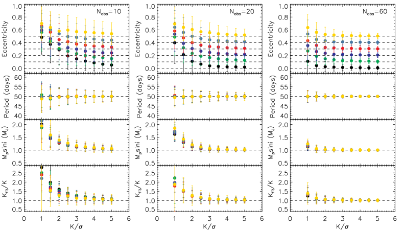
Figure 1.— Effects of signal-to-noise ratio and number of observations on the best-fit orbital parameters. Filled circles are median values; the true orbital parameters are denoted as horizontal lines (see the text for details), where $\omega$ and temporal offset $t_{0}$ are chosen at random. Error bars show standard deviations. From left to right, $N_{\rm obs}=10,20,60$.

2. Keplerian Fitting to Mock RV Data

We consider single planet detections throughout the paper. Assuming a true orbit (period $P$, eccentricity $e$, minimal planet mass $M_{p}\sin i$, argument of periastron $\omega$, and temporal offset $t_{0}$) and the host star mass $M_{*}$, we generate mock RV data sets with Gaussian errors $\sigma$ as perturbations. For simplicity $\sigma$ is assumed to be the same for all data points in a set, but we relax this assumption later (§4). In practice, $\sigma$ comes from RV measurement errors, stellar jitter and possible existence of multiple planets (e.g., Ford 2006). Following Cumming (2004), we define the signal-to-noise ratio ${\cal R}=K/\sigma$ where $K$ is the semi-amplitude of the theoretical RV curve, and in the limit of $M_{p}\ll M_{*}$ we have (e.g., Cumming et al. 1999),

$$K=\bigg{(}\frac{2\pi G}{P}\bigg{)}^{1/3}\frac{M_{p}\sin i}{M_{*}^{2/3}}\frac{1}{\sqrt{1-e^{2}}}\ .$$ (1)

Here the amplitude $K$ is defined in terms of the intrinsic properties of a planet’s orbit, since we “know” the true orbital parameters in advance.

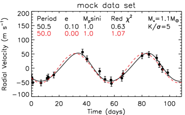
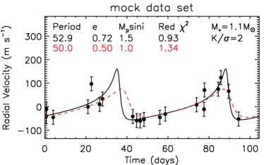
Figure 2.— Left: An example of Keplerian fit to mock data with ${\rm K/\sigma}=5$ and $N_{\rm obs}=20$ where $e_{0}=0$. The perturbed RV data prefer an eccentric orbit over the original circular orbit; but the fitted period and $M_{p}\sin i$ are fairly accurate. Right: An example of large eccentricity orbit fits with $K/\sigma=2$ and $N_{\rm obs}=20$ where $e_{0}=0.5$. In both cases the dashed lines are the RV curves expected from the true orbital parameters while the solid lines are best-fit Keplerian orbits to the data.

In addition to the signal-to-noise ratio ${\cal R}$, another important quantity is the number of observations $N_{\rm obs}$. Clearly the larger ${\cal R}$ and $N_{\rm obs}$ are, the better the quality of the data set.

We consider planets where the orbital period is shorter than the observational time span. Orbits with periods longer than the time baseline are difficult to detect due to limited sampling and lower amplitude (e.g., Cumming 2004). Even if detected, the best-fit orbital solution would often be very different from the true one (Shen et al. 2008, in preparation). The observation times are randomly generated within the observational time span, which somewhat mimics the effects of realistic radial velocity sampling.

In Fig. 1 we plot the relations of fitted eccentricity, period, minimal planet mass and semi-amplitude to their true values, as functions of ${\cal R}$, for a specific case with $M_{*}=1.1\ M_{\odot}$, $P=50$ days, $M_{p}\sin i=1\ M_{J}$, and eccentricity values $e=0.0-0.5$ at intervals of $\Delta e=0.1$. Each set of true orbits was used to generate 5000 mock RV data sets with randomly chosen $\omega$ and temporal offset $t_{0}$, and with Gaussian noise determined from the assumed signal-to-noise ratio. We used the Levenberg-Marquardt method (e.g., Press et al. 1992) to minimize $\chi^{2}$, and the true orbital parameters were used as an initial guess for the $\chi^{2}$ fitting. Using the true orbital parameters as the initial guess greatly speeds up the convergence and increases the rate of successful fits. In the realistic case when we do not know the actual orbital parameters, the success of a fit also depends on an appropriate initial guess. We will come back to this point in §3. The mock observational time span $T$ was set to be two true periods, but we find almost identical results as long as the period is shorter than the time span. Finally, we simulated three values of $N_{\rm obs}=10,20,60$.

Not all attempts to find a Keplerian fit will result in a detection. In an actual radial velocity search for planets, some threshold on the false alarm probability (FAP), the probability that a signal power will arise purely from noise, of a Keplerian fit, is normally used. Throughout the paper we adopt a fiducial ${\rm FAP}=10^{-2}$, which is essentially always satisfied for large $K/\sigma$ and $N_{\rm obs}$. There are several ways to estimate the FAP using Monte Carlo simulations or analytical formulae. For simplicity we have followed the analytical procedure described in Cumming (2004) to estimate the FAP: Given the least-$\chi^{2}$ value $\chi^{2}_{\rm Kep}$ from the Keplerian fit, and the least-$\chi^{2}$ value $\chi^{2}_{\rm mean}$ from the fit of a constant to the data, we calculate a power $z_{0}$ using eqn. (7) in Cumming (2004). An estimate of the FAP is then eqn. (5) in Cumming (2004): ${\rm FAP}=1-[1-{\rm Prob}(z>z_{0})]^{\cal M}$, where ${\cal M}\approx T/T_{\rm min}$ is the number of independent frequencies with $T$ the observational time span and $T_{\rm min}=2$ days the lower bound of period searched in the Keplerian fitting, and ${\rm Prob}(z>z_{0})$ is the probability distribution given by eqn. (8) in that paper.

All three panels in Fig. 1 show that the fitted period is fairly accurate. However, for eccentricity and $M_{p}\sin i$ (and also the amplitude $K$ following eqn. 1) the median fitted values are biased upward, and this behavior remains for true eccentricities as large as $e_{0}\sim 0.8$ in our simulations. This is not a failure of the $\chi^{2}$ minimization method. In Fig. 2 we show two examples of Keplerian fits where both RV data sets prefer a more eccentric orbit. The biases in $e$ and $M_{p}\sin i$, as well as the scatter around the median, decrease when ${\cal R}$ or $N_{\rm obs}$ increases, as would be naively expected.

These fitting biases result from the fact that, in general, the least-$\chi^{2}$ solution is not an unbiased estimator of the true parameters for the non-linear Keplerian model even if the data errors are Gaussian. In particular, the probability distribution ${\cal P}(\mathbf{\hat{\theta}}|\mathbf{\theta})$ is not Gaussian, where $\mathbf{\theta}$ is the set of true parameter and $\mathbf{\hat{\theta}}$ is the best-fit orbital solution; and it only approaches a Gaussian distribution when the errors are small.

To fully take account these biases we need to know ${\cal P}(\mathbf{\hat{\theta}}|\mathbf{\theta})$ for different combinations of $\mathbf{\theta}$, $K/\sigma$ and $N_{\rm obs}$, which can be explored numerically as in Fig. 1. However, for low intrinsic eccentricities ($e_{0}\lesssim 0.5$), the apparent fitting bias in eccentricity can be quantitatively understood as follows. While the error in the fitted eccentricity $\sigma_{e}$ is not Gaussian when $\sigma_{e}$ is comparable to $e$, the fitted $x\equiv e\cos\omega$ and $y\equiv e\sin\omega$ preserve Gaussianity much better provided that the intrinsic eccentricity is small (e.g., Butler et al. 2006). Assuming their fitted values are Gaussian distributions around true values $x_{0}\equiv e_{0}\cos\omega_{0}$ and $y_{0}\equiv e_{0}\sin\omega_{0}$ with dispersion $\sigma_{0}$, the probability distribution of the fitted eccentricity $e$ is given by

$${\cal P}(e) \propto \int\exp\bigg{[}-\frac{(x-x_{0})^{2}}{2\sigma_{0}^{2}}-\frac{(y-y_{0})^{2}}{2\sigma_{0}^{2}}\bigg{]}\delta(e-\sqrt{x^{2}+y^{2}})dxdy$$ (2)

$$\propto e\exp\bigg{(}-\frac{e^{2}}{2\sigma_{0}^{2}}\bigg{)}I_{0}\bigg{(}\frac{ee_{0}}{\sigma_{0}^{2}}\bigg{)}\ ,$$

where $I_{0}$ is the modified Bessel function of the first kind. For circular orbits ($e_{0}=0$) it is a Rayleigh distribution; for eccentric orbits and at the low-dispersion limit ($\sigma_{0}\to 0$) it is approximately a Gaussian distribution.

Figure 3.— Examples of fitted distributions becoming non-Gaussian when the signal-to-noise ratio decreases (see text for the intrinsic parameters). Left: Distributions of fitted $e\cos\omega$ (solid histogram) and $e\sin\omega$ (dotted histogram). Right: Distributions of fitted eccentricities. The median value of fitted eccentricities, denoted as dashed vertical lines, is biased from the intrinsic value $e_{0}=0.1$ in the $K/\sigma=2$ case. The difference between predictions (solid lines) from eqn. (2) and the simulated distributions is due to the fact that the distributions of $e\cos\omega$ and $e\sin\omega$ are not precisely Gaussian.

Fig. 3 shows an example of $[P,e_{0},M_{p}\sin i,\omega_{0},t_{0},M_{*}]=[50,0.1,1,\pi/4,10,1.1]$ with $N_{\rm obs}=60$. For a high signal-to-noise ratio, $K/\sigma=5$ (lower panels), both distributions of fitted eccentricity and $e\cos\omega$ ($e\sin\omega$) are approximately Gaussian. For a low signal-to-noise ratio, $K/\sigma=2$ (upper panels), the eccentricity distribution significantly deviates from a Gaussian while $e\cos\omega$ and $e\sin\omega$ are still distributed in an approximately Gaussian form. We plot the predictions of fitted eccentricity distribution from eqn. (2) as solid lines, using the best-fit Gaussian dispersion of the $e\cos\omega$/$e\sin\omega$ distributions. In this way we can also understand the upward median biases even at intrinsic eccentricities as high as $\sim 0.8$, although the fitted $e\cos\omega$ and $e\sin\omega$ are no longer Gaussian at such high eccentricities–our simulations themselves are more revealing in this case.

A conservative empirical criterion (based on our numerical experiments) for a median bias in fitted eccentricity $\left(\langle e\rangle-e_{0}\right)\lesssim 0.05$ is given by the following joint constraint on $K/\sigma$ and $N_{\rm obs}$:

$$(K/\sigma)N_{\rm obs}^{1/2}\gtrsim 15\ ,$$ (3)

which works reasonably well for $10\leq N_{\rm obs}\leq 200$. This is also an approximate criterion that the median bias in $M_{p}\sin i$ is less than $10\%$. Note again here that $K$ is defined using intrinsic planet properties. In practice, $K$ can only be estimated from the best-fit solution and will on average be overestimated a bit at the low-amplitude end, according to the fitting biases discussed here (e.g., Fig. 1). If using $K_{\rm fit}$ instead, we found a good approximation is to replace equation (3) with

$$(K_{\rm fit}/\sigma)N_{\rm obs}^{1/2}\gtrsim 17\ ,$$ (4)

which compensates the fitting bias of amplitude at the low $K/\sigma$ end.

3. Statistical Models of Orbital Parameter Distributions

We now investigate the selection bias on eccentricity using synthetic RV data sets generated from model distributions of orbital parameters. The detailed comparison of different model distributions and constraints from observational data will be presented in a paper in preparation (Shen et al. 2008). Our purpose here is to investigate the possible selection bias on eccentricity, therefore essentially any well behaved model distributions will do. Nevertheless, we choose a model with physically plausible distributions, as we describe below.

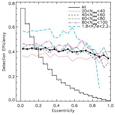
Figure 4.— Colored lines show the detection efficiencies as a function of eccentricity within a given bin of $N_{\rm obs}$. The long-dashed cyan line show the detection efficiency for fixed signal-to-noise ratio. The solid and dashed histograms show the true eccentricity distributions for all the mock orbits and the detected orbits, with the same peak normalization.

The period distribution is a log-normal with log mean of 10 yrs and dispersion of 1 dex. The planet mass $M_{p}$ distribution is a power-law $ndM_{p}\propto M_{p}^{-1}$ within $[0.1,100]\ M_{J}$; this extends well into the “brown dwarf desert” due to the upper limit of $100\ M_{J}$. However such objects are too rare to have any statistical impact on our results. The orientation of the planet orbital plane is random, as is the argument of periastron $\omega$ within $[0,2\pi]$ and the temporal offset $t_{0}$ within one period. For the eccentricity distribution we chose a model that peaks at $e=0$ and diminishes to zero at $e=1$:

$${\cal P}(e)de\propto\bigg{[}\frac{1}{(1+e)^{a}}-\frac{e}{2^{a}}\bigg{]}de\ ,$$ (5)

and we assume $a=4$ for this specific study. Our choice of this particular model distribution is because the peak of the observed eccentricity distribution has shifted from $e\approx 0.2$ to $e\approx 0$ using the latest exoplanet catalog. This model distribution of eccentricity is shown as the solid histogram in Fig. 4. Finally we specify an observational time baseline of $T=10$ years and an overall radial velocity error $\sigma=10\ {\rm m\,s^{-1}}$ for each simulated observation; the number of observations of each object is randomly distributed from $N_{\rm obs}=20$ to $N_{\rm obs}=100$. These parameters are intended to be typical of currently RV surveys (e.g., Cumming et al. 2008).

We generate 100,000 mock orbits of the model distributions and pass them through the Keplerian detection pipeline with a detection threshold ${\rm FAP}=0.01$. For the initial guess of orbital solution, we again take advantage of our mock data sets by using the true orbital parameters. In the realistic case, the initial guess for period can be identified using traditional Lomb-Scargle periodogram (Lomb 1976; Scargle 1982), but appropriate initial guesses for $[e,\omega,t_{0}]$ are crucial for the convergence of Keplerian fits for orbits with high eccentricities, where the fit can easily be trapped in a local minimum due to the complicated $\chi^{2}$ space or fail to converge at all, and hence the planet is undetected. We have run a substantial number of tests, where we tried a fine grid of $[e,\omega,t_{0}]$ as initial guesses in each Keplerian fit. While time consuming, we found that in the vast majority cases the Keplerian fits find the same minimum as using the true parameters as the initial guess. Serendipitous aliasing cases do exist, where the global minimum solution deviates catastrophically from the true orbital parameters, and which are for the most noisy data sets. Hence in the realistic case, special care must be taken to find the global minimum efficiently.

In Fig. 4 we show the overall detection efficiency (the fraction of detected orbits) as function of eccentricity in filled circles, and different line types represent the detection efficiency when binned in $N_{\rm obs}$. Clearly increasing $N_{\rm obs}$ increases the detection efficiency. However, the overall detection efficiency only slowly decreases with eccentricity. This is because although high eccentricity orbits are more difficult to sample, they also have larger amplitude $K$ on average. When we plot the detection efficiency with constant amplitude $K/\sigma\approx 2$, we see a decrease for $e\gtrsim 0.6$, as shown by the cyan long-dashed line in Fig. 4, which is consistent with previous studies (e.g., Endl et al. 2002; Cumming 2004). Therefore, there is no strong selection bias against eccentricity, as demonstrated by the similar (true) eccentricity distributions of the mock orbits and the detected ones in Fig. 4. Note, however, the absolute value of the overall detection efficiency here depends on the model distributions and the quality of the survey (noise level and number of observations).

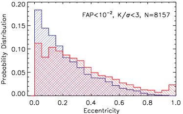
Figure 5.— Low $K/\sigma$ detections for the statistical model (8157 planets detected). Higher and lower histograms show the distributions of the intrinsic and best-fit eccentricities of these detected planets. Shown here is the bias caused by Keplerian fitting: $\sim 40\%$ of the nearly-circular ($e\leq 0.1$) orbits are erroneously assigned to more eccentric orbits by their best fits.

Figure 6.— The effects of Keplerian fitting on the eccentricity distributions. The solid and dashed histograms are the distributions of intrinsic and fitted eccentricities in different $K/\sigma$ and $N_{\rm obs}$ bins. All planets are detected by the Keplerian fitting pipeline, and the numbers of detected planets are listed at the top-right corner of each panel. Those bins with the lowest $K/\sigma$ and $N_{\rm obs}$ are the most seriously affected by the fitting bias.

However, as we have shown in §2, $\chi^{2}$ Keplerian fits will have non-negligible effects for low amplitude detections and therefore bias the underlying eccentricity distribution. Although the detection efficiency decreases rapidly when $K/\sigma$ decreases, there are also many more objects in the low amplitude regime given our model distributions and noise level. We show this bias effect in Fig. 5, where the blue and red histograms show the distributions of true and fitted eccentricities for low amplitude detections with $K/\sigma<3$. The small pile up of fitted $e\gtrsim 0.9$ orbits is caused by detections with period longer than the observation time where the Keplerian fits failed badly (Shen et al. 2008, in preparation). Other than that, the overall effect of the Keplerian fitting bias is the transfer of true low-eccentricity orbits to fitted high-eccentricity ones, therefore distorting the underlying eccentricity distribution. As expected from our simulations in §2, this effect diminishes when we shift to high amplitude and/or large $N_{\rm obs}$ detections, as shown in Fig. 6.

Figure 7.— Inspection of the exoplanet catalog as of January 26, 2008 with $P<20$ days planets excluded. The histogram shows the distribution of $(K_{\rm fit}/\sigma)N_{\rm obs}^{1/2}$ for these planets. We have used the RMS residual of each model fit as an estimate for $\sigma$. The vertical dashed line is at $(K_{\rm fit}/\sigma)N_{\rm obs}^{1/2}=17$, which is the approximate bound below which the best-fit eccentricity is affected by the fitting bias (e.g., eqn. 4).

Figure 8.— An example of the Kepler fits to RV data in the Butler06 catalog (HD 114729b). This particular case has $N_{\rm obs}=42$ and median $K_{\rm fit}/\sigma\approx 3.5$, where $\sigma$ is estimated from the published RV measurement errors and stellar jitter.

4. Discussion

Our results lead naturally to the question of how much bias in the eccentricity distribution is to be expected in the Butler et al. (2006) catalog. To test this we take their updated catalog as of January 26, 2008. We exclude those planets with orbital periods less than 20 days (i.e., those probably have been tidally circularized). Over half of the planets in that catalog do not have published RV data and measurement errors/stellar jitter information, so we use the RMS scatter of the model fit as an estimate of the noise $\sigma$. We also take the amplitude $K$ as the best-fit value $K_{\rm fit}$. There are $162$ planets with $K_{\rm fit}$, ${\rm RMS\ scatter}$ and $N_{\rm obs}$ available. In Fig. 7 we show the distribution of $(K_{\rm fit}/\sigma)N_{\rm obs}^{1/2}$ defined in equation (4) for these planets. There are 19 planets with $(K_{\rm fit}/\sigma)N_{\rm obs}^{1/2}<17$. Thus statistically speaking, only $\sim 10\%$ of the planets are affected in the current sample, which are predominately low-amplitude detections.

To test the effects of unequal errors and realistic sampling we take HD 114729b in the Butler06 catalog as an example. It has a best-fit eccentricity $0.167\pm 0.055$ with $K_{\rm fit}/\sigma\approx 3.5$ and $N_{\rm obs}=42$ where we have estimated $\sigma$ using their published RV measurement errors and stellar jitter. The actual RV data and their best-fit solution is shown in Fig. 8. Using the true time series and data uncertainties derived from measurement errors and stellar jitter for this system, but with simulated radial velocities, we find that the probability of a fitted eccentric orbit with $e\geq 0.15$ arising from a circular orbit is $\sim 8\%$, and increases to $20\%$ for a fitted $e\geq 0.1$, consistent with our results in §2 with constant uncertainties and random sampling.

5. Conclusions

We have performed simulations of planet detection and orbital parameter fits using mock radial velocity data sets. Two effects that may affect the intrinsic eccentricity distribution are considered: selection bias on eccentricity, and fitting bias in the best-fit orbital solution.

We find that selection bias on eccentricity is negligible, as long as the fitting routine is efficient in finding the global solution. In a realistic survey, this requires a thorough search in the parameter space, and/or with advanced algorithms optimized for the search. Our finding is not in conflict with previous studies (e.g., Endl et al. 2002; Cumming 2004), which claim that the detection efficiency decreases for $e\gtrsim 0.6$. This is because in previous studies, the detection efficiency as a function of eccentricity is estimated at fixed $K$ while in our study $K$ is larger for more eccentric orbits when other parameters are fixed. On the other hand, we find that for detections with low signal-to-noise ratio and small number of observations, the best-fit eccentricity is biased upward in the median value, which then gives rise to a change in the eccentricity distribution from the intrinsic one.

Inspection of the current exoplanet sample shows only $\sim 10\%$ are likely to be significantly affected by the Keplerian fitting bias. However, future radial velocity surveys will contain an increasing number of low amplitude detections if the number of low mass, large semi-major axis exoplanets grows as rapidly as suggested by extrapolation of current results suggest (e.g., Udry & Santos 2007). When the sample of low amplitude detections (on average less massive planets and more circular orbits) is large enough for statistical study, the bias in the best-fit eccentricity described here must be taken into account. Also, in individual cases where an accurate estimate of eccentricity is required, i.e., in modeling the habitable zone or tidal heating issues, either high quality RV data or constraints from other observations are required to support reliable conclusions. In the mean time, there is also a need for a more statistically sophisticated understanding of the uncertainties of derived orbital solutions (e.g., Ford 2005; 2006).

Our results suggest that the intrinsic eccentricity distribution may be even more peaked at $e\approx 0$ than the current observed distribution. Some planet-planet scattering models tend to produce a Rayleigh-distribution of eccentricities (e.g., Juric & Tremaine 2007; Ford & Rasio 2007) with reduced circular orbits, therefore certain eccentricity damping mechanism such as interactions with a protoplanetary disk may be required to reconcile these models with observations.

References

- (1) Butler, R. P., et al. 2006, ApJ, 646, 505 (Butler06)
- (2) Cumming, A. 2004, MNRAS, 354, 1165
- (3) Cumming, A., Marcy, G. W., & Butler, R. P. 1999, ApJ, 526, 890
- (4) Cumming, A., Butler, R. P., Marcy, G. W., Vogt, S. S., Wright, J. T. & Fischer, D. A. 2008, PASP, in press, arXiv:0803.3357
- (5) Endl, M. et al. 2002, A&A, 392, 671
- (6) Ford, E. B. 2005, AJ, 129, 1706
- (7) Ford, E. B. 2006, ApJ, 642, 505
- (8) Ford, E. B., & Rasio, F. A. 2007, ApJ, submitted, arXiv:astro-ph/0703163
- (9) Jones, H. R. A., et al. 2006, MNRAS, 369, 249
- (10) Jurić, M., & Tremaine, S. 2007, ApJ, submitted, arXiv:astro-ph/0703160
- (11) Lomb, N. R. 1976, Ap&SS, 39, 447
- (12) Press, W. H., Teukolsky, S. A., Vetterling, W. T., & Flannery, B. P. 1992, Numerical Recipes (New York: Cambridge Univ. Press)
- (13) Scargle, J. D. 1982, ApJ, 263, 835
- (14) Tremaine, S., & Zakamska, N. L. 2004, in AIP Conf. Proc. 713, The Search for Other Worlds, ed. S. S. Holt & D. Deming (New York: AIP), 243
- (15) Udry, S., & Santos, N. C. 2007, ARA&A, 45, 397
- (16) Zhou, J.-L., Lin, D. N. C., & Sun, Y.-S. 2007, ApJ, 666, 423