Phase Transition and Separation for Mixture of Liquid He-3 and He-4

Abstract

This article introduces a dynamical Ginzburg-Landau phase transition/separation model for the mixture of liquid helium-3 and helium-4, using a unified dynamical Ginzburg-Landau model for equilibrium phase transitions. The analysis of this model leads to three critical length scales $L_{1}<L_{2}<L_{3}$, detailed theoretical phase diagrams and transition properties with different length scales of the container.

I Introduction

Landau’s legacy on phase transition has been a singular driving force for our recent work on developing a general dynamic transition theory and a unified approach for both equilibrium and non-equilibrium dynamic phase transitions. We hope that the work in this paper is in the spirit of Landau’s legacy.

Superfluidity is a phase of matter in which ”unusual” effects are observed when liquids, typically of helium-4 or helium-3, overcome friction by surface interaction when at a stage, known as the ”lambda point” for helium-4, at which the liquid’s viscosity becomes zero.

The main objectives of this article is to study $\lambda$-phase transitions of liquid helium-4 and and phase separations between liquid helium-3 and liquid helium-4 from both the modeling and analysis points of view.

In the late 1930s, Landau proposed a mean field theory of continuous phase transitions. With the successful application of the Ginzburg-Landau theory to superconductivity, it is nature to transfer something similar to the superfluidity case, as the superfluid transitions in liquid ³He and ⁴He are of similar quantum origin as superconductivity. Unfortunately, we know that the classical Ginzburg-Landau free energy is poorly applicable to liquid helium in a quantitative sense, as described in by Ginzburg in ginzburg .

As an attempt for this challenge problem, we introduces a dynamical Ginzburg-Landau phase transition/separation model for the mixture of liquid helium-3 and helium-4. In this model, we use an order parameter $\psi$ for the phase transition of liquid ⁴He between the normal and superfluid states, and the mol fraction $u$ for liquid ³He. As $u$ is a conserved quantity, a Cahn-Hilliard type equation is needed for $u$, and a Ginzburg-Landau type equation is needed for the order parameter. The interactions of this quantities are built into the system naturally by using a unified dynamical Ginzburg-Landau model for equilibrium phase transitions, where the dynamic model is derived as a a gradient-type flow as outlined in the appendix.

This analysis of the model established enables us to give a detailed study on the $\lambda$-phase transition and the phase separation between liquid ³He and ⁴He. In particular, we derived three critical length scales $L_{1}<L_{2}<L_{3}$ and the corresponding $\lambda$-transition and phase separation diagrams. The derive theoretical phase diagrams based on our analysis agree with classical phase diagram, as shown e.g. in Reichl reichl and Onuki onuki , and it is hoped that the study here will lead to a better understanding of mature of superfluids. Finally, we remark that the order of second transition is mathematically more challenging, and will be reported elsewhere.

One important new ingredient for the analysis is a new dynamic transition theory developed recently by the authors chinese-book ; b-book . With this theory, we derive a new dynamic phase transition classification scheme, which classifies phase transitions into three categories: Type-I, Type-II and Type-III, corresponding respectively to the continuous, the jump and mixed transitions in the dynamic transition theory.

II Model for Liquid Mixture of ³He -⁴He

Liquid ³He and ⁴He can be dissolved into each other. When ³He -atoms are dissolved in liquid ⁴He and the density of ³He increases, the $\lambda$-transition temperature $T_{\lambda}$ decreases; see the liquid mixture phase diagram of ³He -⁴He (Figure 1), where $X=n_{3}/(n_{3}+n_{4}),n_{3}$ and $n_{4}$ are the atom numbers of ³He and ⁴He respectively. When $X=0,T_{\lambda}=2.17K$, where $\lambda$-phase transition takes place and liquid ⁴He undergoes a transition to superfluid phase from the normal liquid phase. When $X=0.67$ and temperature decreases to $T=0.87K$, i.e., at the triple point $C$ in Figure 1, the liquid mixture of ³He -⁴He has a phase separation.

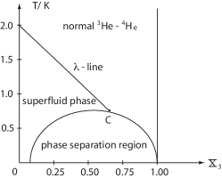
Figure 1: Liquid mixture phase diagram of ³He -⁴He .

Let the complex valued function $\psi=\psi_{1}+i\psi_{2}$ describe the superfluidity of ⁴He, and $u$ be the density of ³He, which is conserved, i.e.,

$$\int_{\Omega}udx=c\ \ \ \ (c>0\ \text{is\ a\ fixed\ number}).$$ (1)

The Ginzburg-Landau (Gibbs) free energy is taken in the following form:

$$G(\psi,\rho_{n},u)= \int_{\Omega}\Big{[}\frac{k_{1}h^{2}}{2m}|\nabla\psi|^{2}+\frac{\gamma_{1}}{2}|\psi|^{2}+\frac{\gamma_{2}}{4}|\psi|^{4}+\frac{k_{2}}{2}|\nabla u|^{2}+\frac{\nu_{1}}{2}u^{2}-\frac{\nu_{2}}{3}u^{3}+\frac{\nu_{3}}{4}u^{4}+\nu_{4}u|\psi|^{2}\Big{]}dx.$$ (2)

where $h$ is the Planck constant, $m$ is the mass of helium-4 atom, and the coefficients satisfy

$$k_{1},k_{2},\gamma_{2},\nu_{2},\nu_{3},\nu_{4}>0.$$ (3)

When $\psi=0$, the liquid mixture of helium-3 and helium-4 is a binary system, and $G(0,u)$ stands for the Cahn-Hilliard free energy. By the standard model (35), from (1) and (2), the equations governing liquid mixture of ³He -⁴He are given as follows:

$$\frac{\partial\psi}{\partial t}=\frac{k_{1}h^{2}}{m}\Delta\psi-\gamma_{1}\psi-\gamma_{2}|\psi|^{2}\psi-2\nu_{4}u\psi,$$ (4)

$$\frac{\partial u}{\partial t}=-k_{2}\Delta^{2}u+\Delta\big{[}\nu_{1}u-\nu_{2}u^{2}+\nu_{3}u^{3}+\nu_{4}|\psi|^{2}\big{]}.$$

These equations have a physically sound constant steady state solution given by

$$(\psi,u)=(0,u^{0}),$$

where $u^{0}>0$ is the density of helium-3 in a homogeneous state. For simplicity, we assume the total density $\rho=1$. Then the system control parameter $X$, the mol fraction of ³He, becomes

$$X=u^{0}\qquad\text{ with }0\leq X\leq 1.$$

Now we consider the derivations from this basic state:

$$(\psi,u)=(\psi^{\prime},X+u^{\prime}),$$

and we derive the following equations (drop the primes):

$$\frac{\partial\psi}{\partial t}=\mu_{1}\Delta\psi-\lambda_{1}\psi-\gamma_{2}|\psi|^{2}\psi-2\nu_{4}u\psi,$$ (5)

$$\frac{\partial u}{\partial t}=-\mu_{2}\Delta^{2}u+\lambda_{2}\Delta u+\Delta[(-\nu_{2}+3\nu_{3}X)u^{2}+\nu_{3}u^{3}+\nu_{4}|\psi|^{2}],$$

$$\int_{\Omega}udx=0,$$

with the Neumann boundary condition

$$\frac{\partial}{\partial n}(u,\Delta u,\psi,\rho_{n})=0\qquad\text{ on }\partial\Omega,$$ (6)

where $mu_{1}=k_{1}h^{2}/m$, $\mu_{2}=k_{2}$, and

$$\lambda_{1}=\gamma_{1}+2\nu_{4}X,$$ (7)

$$\lambda_{2}=\nu_{1}-2\nu_{2}X+3\nu_{3}X^{2}.$$

III Phase Transitions of ³He -⁴He Mixtures

We now apply equations (4) to study the phase transitions of ³He -⁴He liquid mixtures.

III.1 Critical parameter curves

For simplicity we only consider the special case where the container $\Omega$ is a rectangle:

$$\Omega=(0,L)\times(0,l)^{2}\subset\mathbb{R}^{3}\qquad\text{ for }L>l,$$

and the control parameters are the temperature $T$ and the mol fraction $X$, and the length scale $L$ of the container $\Omega$.

Physically, by the Hildebrand theory (see reichl ), in the lower temperature region and at $p=1$ atm, the critical parameter curve $\lambda_{2}=0$ is equivalent to

$$T=\frac{2a}{R}(1-X)X-\sigma_{0},$$ (8)

where $R$ is the molar gas constant and $a>0$ is a constant. Here $\sigma_{0}>0$ is small correction term. The original Hildebrand theory leads to the case where $\sigma_{0}=0$. However, as we can see from the classical phase separation of a binary system, the Hildebrand theory fails when the molar fraction is near $0$ or $1$, and the correction term added here agrees with the experimental phase diagram as shown e.g. in Figure 4.13 in Reichl reichl .

Furthermore, by (7) and (8), we have

$$\nu_{1}\simeq\theta_{1}(T+\sigma_{0}),\quad 3\nu_{3}\simeq 2\nu_{2},\quad\frac{2\nu_{2}}{\theta_{1}}\simeq\frac{2a}{R}.$$ (9)

Consider eigenvalue problem of the linear operator in (5):

$$\left(\begin{matrix}\mu_{1}\Delta-\lambda_{1}&0&0\\ 0&\mu_{1}\Delta-\lambda_{1}&0\\ 0&0&-\Delta(\mu_{2}\Delta-\lambda_{2})\end{matrix}\right)\left(\begin{matrix}\psi_{1}\\ \psi_{2}\\ u\end{matrix}\right)=\beta\left(\begin{matrix}\psi_{1}\\ \psi_{2}\\ u\end{matrix}\right).$$ (10)

Here $\psi=\psi_{1}+\psi_{2}$. It is known that the first eigenvalue and eigenvector of the Laplacian operator with the Neumann condition and zero average are $\lambda=\pi^{2}/L^{2}$ and $u=\cos\pi x_{1}/L$. Thus, the first two eigenvalues and their corresponding eigenvectors of (10) are given by

$$\left\{\begin{aligned} &\beta_{1}=-\lambda_{1}=-(\gamma_{1}+2\nu_{4}X),\\ &(\psi_{1},\psi_{2},u)=(1,0,0)\ \text{and}\ (0,1,0),\end{aligned}\right.$$ (11)

$$\left\{\begin{aligned} &\beta_{2}=-\frac{\pi^{2}}{L^{2}}\left(\frac{\mu_{2}\pi^{2}}{L^{2}}+\lambda_{2}\right)=-\frac{\pi^{2}}{L^{2}}\left(\frac{\mu_{2}\pi^{2}}{L^{2}}+\nu_{1}-2\nu_{2}X+3\nu_{3}X^{2}\right),\\ &(\psi_{1},\psi_{2},u)=(0,0,\cos\pi x_{1}/L).\end{aligned}\right.$$ (12)

As for $\nu_{1}$, the parameter $\gamma_{1}$ is approximately a linear function of $T$. Phenomenologically, we take

$$\gamma_{1}=-\sigma_{1}+\theta_{2}T\qquad(\theta_{2},\sigma_{1}>0).$$ (13)

Then, by (9) and (11)–(13), the critical parameter curves in the $TX$-plane are as follows:

$$l_{1}:\beta_{1}=0\qquad\Longleftrightarrow\qquad T_{c1}=\frac{\sigma_{1}-2\nu_{4}X}{\theta_{2}}=\frac{\sigma_{1}}{\theta_{2}}(1-X),$$ (14)

$$l_{2}:\beta_{2}=0\qquad\Longleftrightarrow\qquad T_{c2}=\frac{2a}{R}X\left(1-X\right)-\sigma_{0}-\frac{\mu_{2}\pi^{2}}{\theta_{1}L^{2}}.$$

Here we have assumed that $\sigma_{1}=2\nu_{4}.$ This assumption is true at $X=1$ as required by $T_{c1}=0$ at $X=1$, and is true as well at other values of $X$ as we approximately take $\sigma_{1}$ and $\nu_{4}$ as constants.

The critical parameter curve $l_{1}$ $(\beta_{1}=0)$ is as shown in Figure 2(a). Let

$$L_{0}=\sqrt{\frac{\mu_{1}\pi^{2}}{\theta_{1}\left(\frac{a}{2R}-\sigma_{0}\right)}}\qquad\qquad\left(\sigma_{0}<\frac{a}{2R}\right),$$ (15)

then when $L>L_{0}$ the critical parameter curve $l_{2}$ $(\beta_{2}=0)$ is as shown in Figure 2(b).

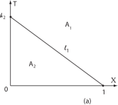
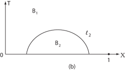
Figure 2: (a) $\beta_{1}<0$ in region $A_{1}$, and $\beta_{1}>0$ in $A_{2}$, (b) $\beta_{2}<0$ in region $B_{1}$, and $\beta_{2}>0$ in $B_{2}$.

III.2 Transition theorems

The following is the transition theorem for liquid mixture ³He -⁴He. Fro this purpose, we introduce a few length scales as follows:

$$L_{1}=\left(\frac{\mu_{2}\pi^{2}}{\theta_{1}}\right)^{1/2}\cdot\frac{1}{\left(\frac{a}{2R}+\frac{2\nu^{2}_{4}}{\theta_{1}\gamma_{2}}-\sigma_{0}\right)^{1/2}}\qquad\qquad\qquad\left(\frac{a}{2R}+\frac{2\nu^{2}_{4}}{\theta_{1}\gamma_{2}}-\sigma_{0}>0\right),$$ (16)

$$L_{2}=\left\{\begin{aligned} &\left(\frac{\mu_{2}\pi^{2}}{\theta_{1}}\right)^{1/2}\cdot\frac{1}{\left[\frac{R}{8a}\left(\frac{2a}{R}-\frac{\sigma_{1}}{\theta_{2}}\right)^{2}+\frac{2\nu_{4}^{2}}{\theta_{1}\gamma_{2}}-\sigma_{0}\right]^{1/2}}&&\text{ if }\frac{R}{8a}\left(\frac{2a}{R}-\frac{\sigma_{1}}{\theta_{2}}\right)^{2}+\frac{2\nu_{4}^{2}}{\theta_{1}\gamma_{2}}>\sigma_{0}\\ &\infty&&\text{ otherwise},\end{aligned}\right.$$ (17)

$$L_{3}=\left\{\begin{aligned} &\left(\frac{\mu_{2}\pi^{2}}{\theta_{1}}\right)^{1/2}\cdot\frac{1}{\left[\frac{R}{8a}\left(\frac{2a}{R}-\frac{\sigma_{1}}{\theta_{2}}\right)^{2}-\sigma_{0}\right]^{1/2}}&&\quad\qquad\text{ if }\frac{R}{8a}\left(\frac{2a}{R}-\frac{\sigma_{1}}{\theta_{2}}\right)^{2}>\sigma_{0}\\ &\infty&&\qquad\quad\text{ otherwise}.\end{aligned}\right.$$ (18)

We remark here again that $\sigma_{0}$ is small as a correction term in the Hildebrand theory as mentioned earlier in (8).

Theorem 1

Let $T_{c1}$ and $T_{c2}$ be given in (14). For equations (5), we have the following assertions:

• When $L<L_{1}$ the system has only the superfluid phase transition (i.e., the $\lambda$-phase transition) at $T=T_{c}^{1}$, and the $TX$-phase diagram is as shown in Figure 2(a).

• Let $\sigma_{1}/\theta_{2}<4a/R$. Then $L_{1}<L_{2}$, and if $L_{1}<L<L_{2}$, then there are two numbers $0<X_{1}<\frac{1}{2}<X_{2}<1$ given by

  $$X_{1,2}=\frac{1}{2}\left[1\pm\sqrt{1+\frac{2R}{a}\left(\frac{2\nu_{4}^{2}}{\theta_{1}\gamma_{2}}-\sigma_{0}-\frac{\mu_{2}\pi^{2}}{\theta_{1}L^{2}}\right)}\right]$$ (19)

  such that the following hold true:

  • if $0\leq X<X_{1}$ or $X_{2}<X<1$, the system has only the $\lambda$-phase transition at $T=T_{c}^{1}$;

  • if $X_{1}<X<X_{2}$, then the system has the $\lambda$-phase transition at $T=T_{c1}$, and has the phase separation at $T^{*}=T_{c2}+\frac{2\nu_{4}^{2}}{\theta_{1}\gamma_{2}}<T_{c1}$. Moreover, the $TX$-phase diagram is as shown in Figure 3.

• Let $\sigma_{1}/\theta_{2}<4a/R$. For any $L_{2}<L<L_{3}$, the phase diagram is as shown in Figure 4. For any $L_{3}<L$, the phase diagram is as shown in Figure 5.

• Let $\sigma_{1}/\theta_{2}\geq 4a/R$. Then for any $L\geq L_{1}$, Assertion (2) holds true.

• The $\lambda$-phase transition at $T=T_{c}^{1}$ is Type-I, which corresponds to second-order transition.

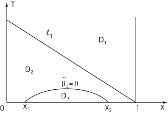
Figure 3: Region $D_{1}$ is normal ³He -⁴He , $D_{2}$ is the superfluid phase, and $D_{3}$ is the phase separation region.

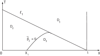
Figure 4: Region $D_{1}$ is normal ³He -⁴He , $D_{2}$ is the superfluid phase, and $D_{3}$ is the phase separation region.

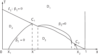
Figure 5: Region $D_{1}$ is normal ³He -⁴He , $D_{2}$ is the superfluid phase, and $D_{3}$ is the phase separation region.

It is worth mentioning that the order of second transitions crossing $\widetilde{\beta}_{1}=0$ is an interesting problem, which will be analyzed in a forthcoming paper.

Proof of Theorem 1. We proceed in several steps as follows.

Step 1. It is easy to see that the space

$$E=\{(u,\psi)=(0,\psi)|\ \psi\in\mathbb{C}\}$$

is invariant for (5). Therefore, the transition solutions of (5) from the critical parameter curve $l_{1}$ $(\lambda_{1}=0)$ must be in $E$, which corresponds to the superfluid transition. On the other hand, restricted on $E$, equations (4) are equivalent to the following ordinary differential equation:

$$\frac{d\psi}{dt}=-\lambda_{1}\psi-\gamma_{2}|\psi|^{2}\psi.$$ (20)

It is then easy to see that Assertion (5) holds true, and the bifurcated solutions consist of a circle given by

$$\{\sqrt{-\lambda_{1}/\gamma_{2}}\ e^{i\phi}\ |\ \phi\in[0,2\pi]\}.$$

Step 2. We now consider the second transition. For this purpose, let the transition solution of (4) from $T=T_{c}^{1}$ (i.e., from $\lambda_{1}=0)$ be given by

$$(0,\widetilde{\psi}(T))=(0,\sqrt{-\lambda_{1}/\gamma_{2}}\ e^{i\phi})\in E.$$ (21)

Take the transition

$$(u,\psi)\rightarrow(u^{\prime},\psi^{\prime}+\widetilde{\psi}).$$

Then the equations (5) are rewritten as (drop the primes)

$$\frac{\partial\psi}{\partial t}=\mu_{1}\Delta\psi+\lambda_{1}\psi+\lambda_{1}\psi^{\ast}-2\nu_{4}\sqrt{\frac{-\lambda_{1}}{\gamma_{2}}}u-2\gamma_{2}\sqrt{\frac{-\lambda_{1}}{\gamma_{2}}}|\psi|^{2}-2\nu_{4}u\psi-\gamma_{2}|\psi|^{2}\psi,$$ (22)

$$\frac{\partial u}{\partial t}=-\mu_{2}\Delta^{2}u+\lambda_{2}\Delta u+2\nu_{4}\sqrt{\frac{-\lambda_{1}}{\gamma_{2}}}\Delta\psi_{1}+\Delta[(-\nu_{2}+3\nu_{3}X)u^{2}+\nu_{3}u^{3}+\nu_{4}|\psi|^{2}],$$

$$\int_{\Omega}udx=0,$$

where $\psi=\psi_{1}+i\psi_{2}$

We consider the transition of (22) beyond $E$. The linear operator of (22) is given by

$$B=\left(\begin{matrix}2\lambda_{1}&0&-2\nu_{4}\sqrt{\frac{-\lambda_{1}}{\gamma_{2}}}\\ &&\\ 0&\lambda_{1}&0\\ &&\\ 2\nu_{4}\sqrt{\frac{-\lambda_{1}}{\gamma_{2}}}\Delta&0&\Delta(-\mu_{2}\Delta+\lambda_{2})\end{matrix}\right).$$ (23)

Restricted to its first eigenspace

$$E_{1}=\left\{(\psi_{1},\psi_{2},u)=(y_{1},y_{2},y_{3})\cos\frac{\pi x_{1}}{L}\ |\ (y_{1},y_{2},y_{3})\in\mathbb{R}^{3}\right\},$$

the linear $B$ is given by

$$B|_{E_{1}}=\left(\begin{matrix}2\lambda_{1}&0&-2\nu_{4}\sqrt{\frac{-\lambda_{1}}{\gamma_{2}}}\\ &&\\ 0&\lambda_{1}&0\\ &&\\ -\frac{2\nu_{4}\pi^{2}}{L^{2}}\sqrt{\frac{-\lambda_{1}}{\gamma_{2}}}&0&-\frac{\pi^{2}}{L^{2}}(\frac{\mu_{2}\pi^{2}}{L^{2}}+\lambda_{2})\end{matrix}\right).$$ (24)

The eigenvalues $\widetilde{\beta}_{1}$, $\widetilde{\beta}_{2}$ and $\widetilde{\beta}_{3}$ of $B|_{E_{1}}$ are given by

$$\widetilde{\beta}_{1,2}=\lambda_{1}-\frac{\pi^{2}}{2L^{2}}\left[\frac{\mu_{2}\pi^{2}}{L^{2}}+\lambda_{2}\right]\pm\sqrt{\left[\lambda_{1}-\frac{\pi^{2}}{2L^{2}}\left(\frac{\mu_{2}\pi^{2}}{L^{2}}+\lambda_{2}\right)\right]^{2}+\frac{2\lambda_{1}\pi^{2}}{L^{2}}\left(\frac{\mu_{2}\pi^{2}}{L^{2}}+\lambda_{2}-\frac{2\nu_{4}^{2}}{\gamma_{2}}\right)},$$

$$\widetilde{\beta}_{3}=\lambda_{1}<0.$$

We know that

$$\widetilde{\beta}_{3}<0,\quad\widetilde{\beta}_{2}<\widetilde{\beta}_{1}\qquad\forall T<T_{c1}.$$

By (9), we have

$$\lambda_{2} =\nu_{1}-2\nu_{2}X+3\nu_{3}X^{2}=\theta_{1}(T+\sigma_{0})-2\nu_{2}(1-X)X$$

$$=\theta_{1}\left(T+\sigma_{0}-\frac{2\nu_{2}}{\theta_{1}}X(1-X)\right)$$

$$=\theta_{1}\left(T-T_{c2}\right)-\frac{\nu_{2}\pi^{2}}{L^{2}}$$

Hence the transition curve $\widetilde{\beta}_{1}=0$ is given by

$$\frac{\mu_{2}\pi^{2}}{L^{2}}+\lambda_{2}=\frac{2\nu_{4}^{2}}{\gamma_{2}},$$

which is equivalent to

$$\theta_{1}\left(T-T_{c2}\right)=\frac{2\nu_{4}^{2}}{\gamma_{2}}.$$

Hence the transition curve $\widetilde{\beta}_{1}=0$ is given by

$$\widetilde{\beta}_{1}=0\qquad\Longleftrightarrow\qquad T=T_{c2}+\frac{2\nu_{4}^{2}}{\theta_{1}\gamma_{2}}=\frac{2a}{R}X(1-X)-\sigma_{0}-\frac{\mu_{2}\pi^{2}}{\theta_{1}L^{2}}+\frac{2\nu_{4}^{2}}{\theta_{1}\gamma_{2}}.$$ (25)

Then $L_{1}$ defined by (16) is the critical length scale to make the transition curve $\widetilde{\beta}_{1}=0$ achieving its maximum at $(T,X)=(0,1/2)$.

By definition, it is then easy to see that if $L<L_{1}$, no phase separation occurs at any temperature although phase transition for ⁴He does occur as the temperature decreases below certain critical temperature.

Step 3. Now we calculate the length scale $L_{2}$ where the critical curves $\beta_{1}=0$ and $\widetilde{\beta}_{1}=0$ are tangent to each other, i.e., they interact at exactly one point. By definition, we need to solve $L$ such that the equation

$$\frac{\sigma_{1}}{\theta_{2}}(1-X)=\frac{2a}{R}X\left(1-X\right)-\sigma_{0}-\frac{\mu_{2}\pi^{2}}{\theta_{1}L^{2}}$$

has exactly one solution. Hence, it is easy to derive that the formula $L_{2}$ is as given by (17).

By comparing $L_{1}$ and $L_{2}$, we have

$$L_{2}>L_{1}\qquad\text{ if and only if }\qquad\frac{\sigma_{1}}{\theta_{2}}<\frac{4a}{R}.$$ (26)

Now we the length scale $L_{3}$ where the critical curves $\beta_{1}=0$ and $\beta_{2}=0$ are tangent to each other, i.e., we need to solve $L$ such that the equation

$$\frac{\sigma_{1}}{\theta_{2}}(1-X)=\frac{2a}{R}X\left(1-X\right)-\sigma_{0}$$

has exactly one solution. The formula $L_{3}$ is as given by (19).

Step 4. Now we return to prove Assertions (1)-(4). First, we consider the case where $\frac{\sigma_{1}}{\theta_{2}}<\frac{4a}{R}$, i.e., $L_{2}>L_{1}$. In this case, for $L_{1}<L<L_{2}$, second transition curve $\widetilde{\beta}_{1}=0$ is as shown in Figure 3. Namely, as one decreases the temperature $T$ entering from region $D_{2}$ into $D_{3}$ through the curve $\widetilde{\beta}_{1}=0$, phase separation occurs.

By (25), solving

$$\frac{2a}{R}X(1-X)-\sigma_{0}-\frac{\mu_{2}\pi^{2}}{\theta_{1}L^{2}}+\frac{2\nu_{4}^{2}}{\theta_{1}\gamma_{2}}=0$$

gives the least and biggest mol fractions $X_{1}<X_{2}$ defined by (19), and Assertion (2) follows. Other assertions can be proved in the same fashion.

The proof of the theorem is complete.   

IV Physical conclusions

We have introduced a dynamical Ginzburg-Landau phase transition/separation model for the mixture of liquid helium-3 and helium-4. In this model, we use an order parameter $\psi$ for the phase transition of liquid ⁴He between the normal and superfluid states, and the mol fraction $u$ for liquid ³He. As $u$ is a conserved quantity, a Cahn-Hilliard type equation is needed for $u$, and a Ginzburg-Landau type equation is needed for the order parameter. The interactions of this quantities are built into the system naturally by using a unified dynamical Ginzburg-Landau model for equilibrium phase transitions, where the dynamic model is derived as a a gradient-type flow as outlined in the appendix.

This analysis of the model established enables us to give a detailed study on the $\lambda$-phase transition and the phase separation between liquid ³He and ⁴He. In particular, we derived three critical length scales $L_{1}<L_{2}<L_{3}$ with the following conclusions:

• For $L<L_{1}$, there is only $\lambda$-phase transition for ⁴He and no phase separation between ³He and ⁴He, as shown in Figure 2(a).

• For $L_{1}<L<L_{2}$, there is no triple points, and phase separation occurs as a second phase transition after the $\lambda$-transition when the mol fraction is between two critical values, as shown in Figure 3.

• For $L_{2}<L<L_{3}$, the $\lambda$-transition is always the first transition, as shown in Figure 4.

• For $L_{3}<L$, both the $\lambda$-transition and the phase separation can appear as either the first transition or the second transition depending on the mol fractions, as shown in Figure 5. In this case, when the phase separation is the first transition, the separation mechanism is the same as a typical binary system as described in great detail by the authors in MW08d .

Also, the $\lambda$-transition is always second-order. The derive theoretical phase diagram based on our analysis agrees with classical phase diagram, and it is hoped that the study here will lead to a better understanding of mature of superfluids. Finally, we remark that the order of second transition is mathematically more challenging, and will be reported elsewhere.

Appendix A Dynamic Ginzburg-Landau models for equilibrium phase transitions

In this section, we recall a unified time-dependent Ginzburg-Landau theory for modeling equilibrium phase transitions in statistical physics; see also MW08f ; MW08c .

Consider a thermal system with a control parameter $\lambda$. By the mathematical characterization of gradient systems and the le Châtelier principle, for a system with thermodynamic potential ${\mathcal{H}}(u,\lambda)$, the governing equations are essentially determined by the functional ${\mathcal{H}}(u,\lambda)$. When the order parameters $(u_{1},\cdots,u_{m})$ are nonconserved variables, i.e., the integers

$$\int_{\Omega}u_{i}(x,t)dx=a_{i}(t)\neq\text{constant}.$$

then the time-dependent equations are given by

$$\left.\begin{aligned} &\frac{\partial u_{i}}{\partial t}=-\beta_{i}\frac{\delta}{\delta u_{i}}{\mathcal{H}}(u,\lambda)+\Phi_{i}(u,\nabla u,\lambda),\end{aligned}\right.$$ (27)

for $1\leq i\leq m$, where $\beta_{i}>0$ and $\Phi_{i}$ satisfy

$$\int_{\Omega}\sum_{i}\Phi_{i}\frac{\delta}{\delta u_{i}}{\mathcal{H}}(u,\lambda)dx=0.$$ (28)

The condition (28) is required by the Le Châtelier principle. In the concrete problem, the terms $\Phi_{i}$ can be determined by physical laws and (28). We remark here that following the le Châtelier principle, one should have an inequality constraint. However physical systems often obey most simplified rules, as many existing models for specific problems are consistent with the equality constraint here. This remark applies to the constraint (34) below as well.

When the order parameters are the number density and the system has no material exchange with the external, then $u_{j}$ $(1\leq j\leq m)$ are conserved, i.e.,

$$\int_{\Omega}u_{j}(x,t)dx=\text{constant}.$$ (29)

This conservation law requires a continuity equation

$$\frac{\partial u_{j}}{\partial t}=-\nabla\cdot J_{j}(u,\lambda),$$ (30)

where $J_{j}(u,\lambda)$ is the flux of component $u_{j}$, satisfying

$$J_{j}=-k_{j}\nabla(\mu_{j}-\sum_{i\neq j}\mu_{i}),$$ (31)

where $\mu_{l}$ is the chemical potential of component $u_{l}$,

$$\mu_{j}-\sum_{i\neq j}\mu_{i}=\frac{\delta}{\delta u_{j}}{\mathcal{H}}(u,\lambda)-\phi_{j}(u,\nabla u,\lambda),$$ (32)

and $\phi_{j}(u,\lambda)$ is a function depending on the other components $u_{i}$ $(i\neq j)$. Thus, from (30)-(32) we obtain the dynamical equations as follows

$$\frac{\partial u_{j}}{\partial t}=\beta_{j}\Delta\left[\frac{\delta}{\delta u_{j}}{\mathcal{H}}(u,\lambda)-\phi_{j}(u,\nabla u,\lambda)\right],$$ (33)

for $1\leq j\leq m$, where $\beta_{j}>0$ are constants, and $\phi_{j}$ satisfy

$$\int_{\Omega}\sum_{j}\Delta\phi_{j}\cdot\frac{\delta}{\delta u_{j}}{\mathcal{H}}(u,\lambda)dx=0.$$ (34)

When $m=1$, i.e., the system is a binary system, consisting of two components $A$ and $B$, then the term $\phi_{j}=0$. The above model covers the classical Cahn-Hilliard model. It is worth mentioning that for multi-component systems, these $\phi_{j}$ play an important rule in deriving good time-dependent models.

If the order parameters $(u_{1},\cdots,u_{k})$ are coupled to the conserved variables $(u_{k+1},\cdots,u_{m})$, then the dynamical equations are

$$\frac{\partial u_{i}}{\partial t}=-\beta_{i}\frac{\delta}{\delta u_{i}}{\mathcal{H}}(u,\lambda)+\Phi_{i}(u,\nabla u,\lambda),$$ (35)

$$\frac{\partial u_{j}}{\partial t}=\beta_{j}\Delta\left[\frac{\delta}{\delta u_{j}}{\mathcal{H}}(u,\lambda)-\phi_{j}(u,\nabla u,\lambda)\right],$$

for $1\leq i\leq k$ and $k+1\leq j\leq m$. Here $\Phi_{i}$ and $\phi_{j}$ satisfy (28) and (34), respectively.

The model (35) we derive here gives a general form of the governing equations to thermodynamic phase transitions, and will play crucial role in studying the dynamics of equilibrium phase transitions in statistical physics.

References

- (1) V. L. Ginzburg, On superconductivity and superfluidity (what i have and have not managed to do), as well as on the ’physical minimum’ at the beginning of the xxi century, Phys.-Usp., 47 (2004), pp. 1155–1170.
- (2) T. Ma and S. Wang, Bifurcation theory and applications, vol. 53 of World Scientific Series on Nonlinear Science. Series A: Monographs and Treatises, World Scientific Publishing Co. Pte. Ltd., Hackensack, NJ, 2005.
- (3) , Stability and Bifurcation of Nonlinear Evolutions Equations, Science Press, 2007.
- (4) , Cahn-hilliard equations and phase transition dynamics for binary systems, Dist. Cont. Dyn. Systs., Ser. B, (2008).
- (5) , Dynamic phase transition theory in PVT systems, Indiana University Mathematics Journal, to appear; see also Arxiv: 0712.3713, (2008).
- (6) , Dynamic phase transitions for ferromagnetic systems, Journal of Mathematical Physics, 49:053506 (2008), pp. 1–18.
- (7) O. Onuki, Phase transition dynamics, Combridge Univ. Press., (2002).
- (8) L. E. Reichl, A modern course in statistical physics, A Wiley-Interscience Publication, John Wiley & Sons Inc., New York, second ed., 1998.