Universal Record Statistics of Random Walks and Lévy Flights

Abstract

It is shown that statistics of records for time series generated by random walks are independent of the details of the jump distribution, as long as the latter is continuous and symmetric. In $N$ steps, the mean of the record distribution grows as the $\sqrt{4N/\pi}$ while the standard deviation grows as $\sqrt{(2-4/\pi)N}$, so the distribution is non-self-averaging. The mean shortest and longest duration records grow as $\sqrt{N/\pi}$ and $0.626508...N$, respectively. The case of a discrete random walker is also studied, and similar asymptotic behavior is found.

The study of record statistics is an integral part of diverse fields including meteorology climate ; RP , hydrology Matalas , economics Barlevy , sports GTS ; Glick ; BRV and entertainment industries among others. In popular media such as television or newspapers, one always hears and reads about record breaking events. It is no wonder that Guinness Book of Records has been a world’s best-seller since 1955. In physics, records are relevant in the theory of domain-wall dynamics ABBM , for example. Consider any discrete time series $\{x_{0},x_{1},x_{2},\ldots,x_{N}\}$ of $N$ entries that may represent, e.g., the daily temperatures in a city or the stock prices of a company or the budgets of Hollywood films. A record happens at step $i$ if the $i$-th entry $x_{i}$ is bigger than all previous entries $x_{0}$, $x_{1}$, $\ldots$, $x_{i-1}$. Statisical questions that naturally arise are: (a) how many records occur in time $N$? (b) How long does a record survive? (c) what is the age of the longest surviving record? etc. Understanding these aspects of record statistics is particularly important in the context of current issues of climatology such as global warming.

The mathematical theory of records has been studied for over 50 years Chandler ; Nevzorov ; ABN ; SZ and the questions posed in the previous paragraph are well understood in the case when the random variables $x_{i}$’s are independent and identically distributed (iid). Recently, there has been a resurgence of interest in the record theory due to its multiple applications in diverse complex systems such as spin glasses SG , adaptive processes Orr and evolutionary models of biological populations Krug1 ; Evol . The results in the record theory of iid variables have been rather useful in these different contexts. Recently, Krug has studied the record statistics when the entries have non-identical distributions but still retain their independence Krug2 . However, in most realistic situations the entries of the time series are correlated. Surprisingly, very little is known about the statistics of records for a correlated time series. In this Letter we take a step towards this goal.

Of correlated time series $\{x_{0},x_{1},x_{2},\ldots,x_{N}\}$, perhaps the simplest and yet the most common with a variety of applications Feller , is the one where $x_{i}$ represents the position of a random walker at discrete time $i$. The walker starts at $x_{0}$ at time $0$ and at each discrete step evolves via $x_{i}=x_{i-1}+\eta_{i}$ where the noise $\eta_{i}$ represents the jump length at step $i$. The jump lengths $\eta_{i}$’s are iid variables each drawn from a symmetric distribution $\phi(\eta)$. This also includes Lévy flights where $\phi(\eta)\sim|\eta|^{-1-\mu}$ is power-law distributed for large $|\eta|$ with exponent $0<\mu\leq 2$ and thus has a divergent second moment. Even though the jump lengths are uncorrelated, the entries $x_{i}$’s are clearly correlated. This time series corresponding to a discrete-time Brownian motion appears naturally in many different contexts. For example, in the context of queuing theory queue , $x_{i}$ represents the length of a single queue at time $i$. In the context of the evolution of stock prices $x_{i}$ represents the logarithm of the price of a stock at time $i$ finance . In this Letter, we compute exactly the statistics of the number and the ages of records in this correlated sequence and show that the record statistics is universal, i.e., independent of the noise distribution $\phi(\eta)$ as long as $\phi(\eta)$ is symmetric and continuous.

It is useful to summarize our main results. The record statistics are independent of the starting position $x_{0}$ and hence without any loss of generality we will set $x_{0}=0$ and also count the initial entry $x_{0}=0$ as the first record. We show that the probability $P(M,N)$ of $M$ records in $N$ steps ($M\leq N+1$) is simply

$$P(M,N)=\binom{2N-M+1}{N}\,2^{-2N+M-1}$$ (1)

which is universal for all $M$ and $N$. The moments are also naturally universal and can be computed for all $N$. In particular, for large $N$, the mean and the variance behave as

$$\langle M\rangle \sim \frac{2}{\sqrt{\pi}}\sqrt{N}$$

$$\langle M^{2}\rangle-{\langle M\rangle}^{2} \sim 2\left(1-\frac{2}{\pi}\right)\,N$$ (2)

while the skewness, defined as the third central moment divided by the variance raised to the 3/2-power, goes to a constant value $4(4-\pi)(2\pi-4)^{-3/2}$. We also show that the age statistics of the records is universal for all $N$. Evidently, the mean age of a typical record grows, for large $N$, as $\langle l\rangle\sim N/\langle M\rangle\sim\sqrt{\pi N/4}\approx 0.8862\,\sqrt{N}$. We also compute the extreme age statistics, i.e., ages of the records that have respectively the shortest and the longest duration. These extreme statistics are also universal. While the mean longevity of the record with the shortest age grows, for large $N$, as $\langle l_{\rm min}\rangle\sim\sqrt{N/\pi}\approx 0.5642\,\sqrt{N}$, that of the longest age grows faster, $\langle l_{\rm max}\rangle\sim c\,N$ where $c$ is a nontrivial universal constant

$$c=2\int_{0}^{\infty}dy\,\log\left[1+\frac{1}{2\sqrt{\pi}}\,\Gamma(-1/2,y)\right]=0.626508\ldots$$ (3)

where $\Gamma(-1/2,y)=\int_{y}^{\infty}dx\,x^{-3/2}\,e^{-x}$. The universality of these results can be traced back to the Sparre Andersen theorem on the first-passage property of random walks.

Let us consider any realization of the random walk sequence $\{x_{0}=0,x_{1},x_{2},\ldots,x_{N}\}$ (see Fig. 1), where $x_{i}=x_{i-1}+\eta_{i}$ and $\eta_{i}$’s are iid variables each drawn from the distribution $\phi(\eta)$. Let $M$ be the number of records in this realization. Let ${\vec{l}}=\{l_{1},l_{2},\ldots,l_{M}\}$ denote the time intervals between successive records. Thus $l_{i}$ is the age of the $i$-th record, i.e., it denotes the time up to which the $i$-th record survives. Note that the last record, i.e., the $M$-th record, still stays a record at the $N$-th step since there are no more record breaking events after it. Our aim is to first calculate the joint probability distribution $P\left(\vec{l},M|N\right)$ of the ages $\vec{l}$ and the number $M$ of records, given the length $N$ of the sequence. For this, we need two quantities as inputs. First, let $q(l)$ denote the probability that a walk, starting initially at $x$, stays above (or below) its starting position $x$ up to step $l$. Clearly $q(l)$ does not depend on the starting position $x$. A nontrivial theorem due to Sparre Andersen SA states that $q(l)=\binom{2l}{l}2^{-2l}$ is universal for all $l$, i.e., independent of $\phi(\eta)$ as long as $\phi(\eta)$ is symmetric and continuous. Its generating function is simply

$${\tilde{q}}(z)=\sum_{l=0}^{\infty}q(l)\,z^{l}=\frac{1}{\sqrt{1-z}}.$$ (4)

Our second input is the first-passage probability $f(l)$ that the walker crosses its starting point $x$ for the first time between steps $(i-1)$ and $i$. Evidently, $f(l)=q(l-1)-q(l)$ with $l\geq 1$ is also universal and its generating function is

$${\tilde{f}}(z)=\sum_{l=1}^{\infty}f(l)z^{l}=1-(1-z){\tilde{q}}(z)=1-\sqrt{1-z}.$$ (5)

Figure 1: A realization of the random-walk sequence $\{x_{0}=0,x_{1},x_{2},\ldots,x_{N}\}$ of $N$ steps with $M$ records. Records are shown as black dots. $\{l_{1},l_{2},\ldots,l_{M}\}$ denotes the time intervals between successive records.

Armed with these two ingredients $q(l)$ and $f(l)$, one can then write down explicitly the joint distribution of the ages $\vec{l}$ and the number $M$ of records

$$P\left(\vec{l},M|N\right)=f(l_{1})\,f(l_{2})\,\ldots f(l_{M-1})\,q(l_{M})\,\delta_{{\sum_{i=1}^{M}l_{i},\,N}}$$ (6)

where we have used the Markov property of random walks which dictates that the successive intervals are statistically independent, subject to the global sum rule that the total interval length is $N$ (see Fig. 1). Note that since the $M$-th record is the last one (i.e., no more records have happened after it), the interval to its right has distribution $q(l)$ rather than $f(l)$. One can check that $P\left(\vec{l},M|N\right)$ is normalized to unity when summed over $\vec{l}$ and $M$. Since $q(l)$ and $f(l)$ are universal due to the Sparre Andersen theorem, it follows that $P\left(\vec{l},M|N\right)$ and any of its marginals are also universal.

Let us first compute the probability of the number of records $M$, $P(M|N)=\sum_{\vec{l}}P\left(\vec{l},M|N\right)$. To perform this sum, it is easier to consider its generating function. Multiplying Eq. (6) by $z^{N}$ and summing over $\vec{l}$, one gets

$$\sum_{N=M-1}^{\infty}P(M|N)z^{N}=[{\tilde{f}}(z)]^{M-1}{\tilde{q}}(z)=\frac{(1-\sqrt{1-z})^{M-1}}{\sqrt{1-z}}.$$ (7)

By expanding in powers of $z$ and computing the coefficient of $z^{N}$, we get our first result in Eq. (1). One can also easily derive the moments of $M$ from Eq. (7). For example, for the first three moments we get

$$\langle M\rangle = (2N+1)\,\binom{2N}{N}\,2^{-2N}$$

$$\langle M^{2}\rangle = 2N+2-\langle M\rangle$$

$$\langle M^{3}\rangle = -6N-6+(7+4N)\langle M\rangle.$$ (8)

The large-$N$ behavior in Eq. (2) can then be easily derived from Eq. (8) by using Stirling’s approximation. In Fig. 2, we demonstrate this universality by computing from simulations $\langle M\rangle$ for three different distributions $\phi(\eta)$ (i) uniform in $[-1/2,1/2]$ (ii) Gaussian with zero mean and unit variance and (iii) Cauchy or Lorentzian: $\phi(\eta)={\pi}^{-1}/(1+\eta^{2})$, which is an example of a Lévy flight. We then compare the data with the exact formula in Eq. (8). The agreement is excellent and one cannot distinguish between the four curves for any value of $N$.

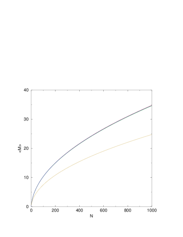
Figure 2: (color online). The top curve actually contains four different curves denoting $\langle M\rangle$ vs $N$ for (i) uniform (ii) Gaussian (iii) Cauchy distributions for $\phi(\eta)$ and also (iv) the exact result in Eq. (8). The four curves are indistinguishable. The bottom curve shows $\langle M\rangle$ vs $N$ for the lattice random walk with $\pm 1$ steps, i.e., when $\phi(\eta)=[\delta_{\eta,1}+\delta_{\eta,-1}]/2$, and agrees with the Eq. (13).

It is also interesting to compare this statistics of $M$ for the random-walk sequence with that of the iid sequence where each entry $x_{i}$ is a random variable drawn from some distribution $p(x)$. In the latter case, it is well known Nevzorov that the distribution of the number of records $P(M|N)$ does not depend on $p(x)$, and for large $N$, it approaches a Gaussian, $P(M|N)\sim\exp[-(M-\log N)^{2}/{2\log N}]$, with mean $\langle M\rangle=\log N$ and the standard deviation $\sigma=\sqrt{\log N}$. Thus, fluctuations of $M$ are small compared to the mean for large $N$. In contrast, for the random-walk sequence, it follows from Eq. (2) that both the mean and the standard deviation grow as $\sqrt{N}$ for large $N$ and thus the fluctuations are large and comparable to the mean. This suggests that in the random-walk case $P(M|N)$ has a scaling form for large $M$ and $N$, $P(M|N)\sim N^{-1/2}\,g(MN^{-1/2})$. One can indeed prove this by analysing Eq.  (7) in the scaling limit and finds $g(x)=e^{-x^{2}/4}/\sqrt{\pi}$.

While the typical age of a record grows as $\langle l\rangle\sim N/\langle M\rangle\sim N^{1/2}$ for large $N$, there are rare records whose ages follow different statistics. For example, what is age distribution of the longest lasting and the shortest lasting records? These extreme statistics of ages can also be derived from the joint distribution in Eq.  (6) and hence they are independent of $\phi(\eta)$.

We first consider the longest lasting record with age $l_{\rm max}={\rm max}(l_{1},l_{2},\ldots,l_{M})$. It is easier to compute its cumulative distribution $F(n|N)$, i.e., the probability that $l_{\rm max}\leq n$ given $N$. Now, if $l_{\rm max}\leq n$, it follows that $l_{i}\leq n$ for $i=1,2,\ldots,M$. Thus, we need to sum up Eq.  (6) over all $l_{i}$’s and $M$ such that $l_{i}\leq n$ for each $i$. As usual it is easier to carry out this summation by considering the generating function and we get

$$\sum_{N}F(n|N)\,z^{N}=\frac{\sum_{l=1}^{n}q(l)z^{l}}{1-\sum_{l=1}^{n}f(l)z^{l}}.$$ (9)

Extracting the distribution $F(n|N)$ from this general expression is somewhat cumbersome and we do not present the details here details . However, one can extract the asymptotic large-$N$ behavior of the average $\langle l_{\rm max}\rangle=\sum_{n=1}^{\infty}[1-F(n|N)]$ from Eq.  (9) using the explicit form of $q(l)$ and $f(l)$. Skipping details details , we find that for large $N$, the mean age of the longest lasting record grows linearly with $N$, $\langle l_{\rm max}\rangle\sim cN$ where $c=0.626508\ldots$ is a universal constant given in Eq.  (3). Thus, the age of the longest record ($\sim N$) is much larger than the typical age ($\sim\sqrt{N}$) for large $N$. Interesingly, exactly the same constant $c$ has appeared before in a different context PitmanYor97 ; Finch08 .

The statistics of the longest record for iid variables follows a similar asymptotic behavior $\langle l_{\rm max}\rangle\sim c_{1}N$ but with the prefactor details

$$c_{1}=\int_{0}^{\infty}dx\exp\left[-x-\int_{x}^{\infty}dy\frac{e^{-y}}{y}\right]=0.624330\ldots$$ (10)

which also describes the asymptotic linear growth of the longest cycle of a random permutation and is known as the Golomb-Dickman or Goncharov’s constant (see Finch03 ). This result for iid variables also emerged recently in the context of a growing network model GL . Interestingly, the constant $c=0.626508..$ for random walks is quite close to the Golomb-Dickman constant. It turns out that although the two problems (iid variables and random walks) have some common features (at least qualitatively), the origin of universality is quite different in the two problems details .

For the record of the shortest duration $l_{\rm min}={\rm min}(l_{1},l_{2},...l_{M})$, one find that the generating function of the cumulative distribution $G(n|N)$ denoting the probability that $l_{\rm min}\geq n$ is given by

$$\sum_{N}G(n|N)\,z^{N}=\frac{\sum_{l=n}^{\infty}q(l)z^{l}}{1-\sum_{l=n}^{\infty}f(l)z^{l}}.$$ (11)

One can then extract, in a similar way, the asymptotic large-$N$ behavior of $\langle l_{\rm min}\rangle\sim\sqrt{N/\pi}$ details . Thus, the mean age of the shortest lasting record grows in a similar way as that of a typical record, albeit with a smaller prefactor $1/\sqrt{\pi}=0.5642\ldots$ compared with $\sqrt{\pi/4}=0.8862\ldots$, respectively.

We have verified the results for $\langle l_{\rm min}\rangle$ and $\langle l_{\rm max}\rangle$ numerically for the case of jump distribution $\phi(\eta)$ uniform in $[-1/2,1/2]$, simulating $10^{9}$ samples containing $10^{4}$ steps each. We kept track of the largest and smallest interval between records (including the final incomplete time interval) for each value of $N$, and calculated the average over all the runs. The results are shown in Fig. 3, where we plot $\langle l_{\rm min}\rangle/\sqrt{N}$ and $\langle l_{\rm max}\rangle/N$, in the first case vs. $1/\sqrt{N}$, and in the second case vs. $1/N$; making plots this way, we find that the data falls on a nearly straight line as $N\to\infty$ in each case. The intercepts, $0.56480$ and $0.62652$, agree closely with the predictions, $\sqrt{1/\pi}=0.564190\ldots$ and $0.626508$, respectively.

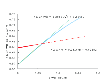
Figure 3: (color online). Plot of simulation results for $\langle l_{\rm min}\rangle/\sqrt{N}$ vs. $1/\sqrt{N}$ (blue data falling on the steeper curve) and $\langle l_{\rm max}\rangle/N$ vs. $1/N$ (red data falling on the less-steep curve), showing the asymptotic behavior of these two quantities. Linear fits to the data for $500<N<10000$ yield the straight lines, whose equations are displayed.

We also considered the discrete (non-continuous) case where the walk jumps by $\eta=\pm 1$ at each time step. For this case we find

$$\sum_{N=0}^{\infty}\langle M\rangle z^{N}=\frac{\sqrt{1+z}+\sqrt{1-z}}{2(1-z)^{3/2}}$$ (12)

which implies

$$\langle M\rangle=\frac{1}{2}\left[1+\frac{(-1)^{N+1}\Gamma(N-\frac{1}{2})_{2}F_{1}(\frac{3}{2},-N;\frac{3}{2}-N;-1)}{2\sqrt{\pi}\Gamma(N+1)}\right]$$ (13)

where ${}_{2}F_{1}$ is the hypergeometric function, implying $\langle M\rangle=1,3/2,7/4,2,35/16$, for $N=0,1,2,3,4$. For large $N$, $\langle M\rangle\sim\sqrt{2N/\pi}$, which is $1/\sqrt{2}$ of the expression for the mean in the continuous case. We also find $\langle l_{\rm max}\rangle\sim cN$, and $\langle l_{\rm min}\rangle\sim\sqrt{2N/\pi}$, which are respectively equal to, and $\sqrt{2}$ times, the corresponding expressions for the continuous case. These results were also verified in a simulation.

In conclusion, we have shown that the record statistics of a time series generated by a Markov process (random walk) are independent of the details of the walk distribution when that distribution is continuous and symmetric. Walks with a discrete jump distribution show similar asymptotic behavior but in general with different coefficients. The results should be useful in analyzing a broad class of physical phenomena and are relevant for example to analyzing questions of climate change. A possible future problem is the calculation of record statistics for non-symmetric random jumps (with a drift) – such as would be the case for a global warming trend.

Support of the National Science Foundation under Grant No. DMS-0553487 is gratefully acknowledged (RMZ). Useful comments by Steven Finch are highly appreciated.

References

- (1) D. V. Hoyt, Climate Change 3, 243 (1981); R. E. Benestad, Climate Research 25, 3 (2003).
- (2) S. Redner and M. R. Petersen, Phys. Rev. E 74, 061114 (2006).
- (3) N. C. Matalas, Climate Change 37, 89 (1997); R. M. Vogel, A. Zafirakou-Koulouris, and N. C. Matalas, Water Res. Research 37, 1723 (2001).
- (4) G. Barlevy, Review of Economic Studies 69, 65 (2002); G. Barlevy and H. N. Nagaraja, J. Appl. Prob. 43, 1119 (2006).
- (5) D. Gembris, J. G. Taylor, and D. Suter, Nature 417, 506 (2002).
- (6) N. Glick, Amer. Math. Monthly 85, 2 (1978).
- (7) E. Ben-Naim, S. Redner, and F. Vazquez, Europhys. Lett. 77, 30005 (2007).
- (8) B. Alessandro, C. Beatrice, G. Bertotti, and A. Montorsi, J. Appl. Phys. 68, 2901 (1990).
- (9) K. N. Chandler, J. Roy. Stat. Soc. Ser. B 14, 220 (1952).
- (10) V. B. Nevzorov, Theory Probab. Appl. 32, 201 (1987).
- (11) B. C. Arnold, N. Balakrishnan, and H. N. Nagaraja, Records (New York, Wiley, 1998).
- (12) B. Schmittmann and R. K. P. Zia, Am. J. Phys. 67, 1269 (1999).
- (13) P. Sibani and P. B. Littlewood, Phys. Rev. Lett. 71, 1482 (1993); P. E. Andersen, H. J. Jensen, L. P. Oliveira, and P. Sibani, Complexity, 10, 49 (2004).
- (14) H. A. Orr, Nature Rev. Gen. 6, 119 (2005).
- (15) J. Krug and C. Karl, Physica A 318, 137 (2003); J. Krug and K. Jain, Physica A 358, 1 (2005); K. Jain and J. Krug, J. Stat. Mech. P04008 (2005).
- (16) E. Ben-Naim and P. L. Krapivsky, J. Stat. Mech. L10002 (2005); C. Sire, S. N. Majumdar, and D. S. Dean, J. Stat. Mech. L07001 (2006); I. Bena and S. N. Majumdar, Phys. Rev. E 75, 051103 (2007).
- (17) J. Krug, J. Stat. Mech. P07001 (2007).
- (18) W. Feller An Introduction to Probability Theory and its Applications (New York, Wiley, 1968).
- (19) S. Asmussen, Applied Probability and Queues (New York, Springer, 2003); M. J. Kearney, J. Phys. A 37, 8421 (2004).
- (20) R. J. Williams, Introduction to the Mathematics of Finance (AMS, 2006); M. Yor, Exponential Functionals of Brownain Motion and Related Topics (Berlin, Springer, 2000).
- (21) E. Sparre Andersen, Mathematica Scandinavica 1, 263-285 (1953); 2, 195-223 (1954); see also Feller .
- (22) S. R. Finch, Mathematical Constants (Cambridge University Press, 2003), 284-292.
- (23) J. Pitman and M. Yor, Annals Probab. 25, 855 (1997).
- (24) S. R. Finch, “Excursion durations,” http://algo.inria.fr/bsolve (2008).
- (25) Details will be published elsewhere.
- (26) C. Godreche and J. M. Luck (unpublished).