Shock formation and the ideal shape of ramp compression waves

Abstract

We derive expressions for shock formation based on the local curvature of the flow characteristics during dynamic compression. Given a specific ramp adiabat, calculated for instance from the equation of state for a substance, the ideal nonlinear shape for an applied ramp loading history can be determined. We discuss the region affected by lateral release, which can be presented in compact form for the ideal loading history. Example calculations are given for representative metals and plastic ablators. Continuum dynamics (hydrocode) simulations were in good agreement with the algebraic forms. Example applications are presented for several classes of laser-loading experiment, identifying conditions where shocks are desired but not formed, and where long duration ramps are desired.

I Introduction

Lasers are used increasingly in the study of the response of matter under extreme conditions, by inducing dynamic loading by ablation. The canonical classes of dynamic loading experiment are shocks shockref and ramps rampref . Laser ablation can be used to induce either type of loading by altering the irradiance history of the laser pulse Swift_lice_05 . To a crude approximation, the ablation pressure is proportional to the irradiance Swift_elements_04 , so a square laser pulse induces a shock and a ramped pulse, a ramp. A shock wave propagating through matter has an inherent rise time, related to the nature of the dissipative processes, such as viscosity or scattering, causing the associated increase of entropy. For a simply-behaved material (neglecting or simplifying time-dependent responses such as plastic flow and phase changes), a shock propagates unchanged if the drive supports it for long enough, whereas a ramp of a given rise time progressively steepens as it propagates. Eventually, the rise time reaches the inherent rise time of a shock, and the ramp becomes a shock. Laser pulses generally have a finite rise time even when a shock is intended, so some part of the target material is subjected to a ramp until it steepens to form a shock.

Here we consider the formation of a shock from a ramp, with application to several situations in laser ablation experiments. We consider several different classes of laser-shock experiment, discussed later in more detail, but broadly depending on the pulse energy of the laser. Experimental techniques have been developed furthest for high energy lasers, and here we are interested in understanding how much of the sample is not shocked, for comparisons with microscopic analysis of recovered samples Peralta05 . A current interest is the use of lasers of lower energy that can be transported to other facilities to induce loading which is then probed by other techniques such as synchrotron radiation McNaney08 ; here we want to determine whether any given laser system is capable of producing a shock in any useful part of the sample. Finally, we are interested in the optimization of ramp loading experiments to allow ramp loading to occur over the maximum possible distance before a shock forms.

In principle, all of these situations can be investigated using spatially-resolved continuum dynamics simulations: hydrocode calculations. However, the numerical time-integration algorithms in these simulations are almost universally unstable when the solution contains a shock wave, which is a perfect discontinuity in the continuum approximation. An artificial viscosity is used to smear a shock over several spatial zones Benson92 . The use of shock smearing makes it difficult to study the formation of a shock from a ramp, because it removes the clear distinction between the different types of wave, and the shock formation process may depend on the specific form of artificial viscosity chosen. Here we analyze the steepening of a ramp and the formation of a shock in terms of the characteristics of the flow, which does not require a numerical discretization of space (or time), and allows shock formation to be identified uniquely in the continuum approximation.

As discussed below, the steepening of a ramp compression wave is closely connected with the spreading of a release wave, and can be investigated using the same relations.

II Steepening of a ramp wave

A ramp wave evolves as the region at a given pressure engulfs more material, the incremental compression wave traveling at the instantaneous sound speed $c$. In a material whose equation of state (EOS) is simple, $c$ increases monotonically with pressure $p$. Thus the ramp wave steepens as it propagates. The steepening can be understood in terms of characteristics of the continuum equations, which for a material described by a scalar EOS comprise in one dimension the material (or particle) flow velocity $u$ and sound waves propagating forward and backward with respect to the flow, $u\pm c$. While the flow remains ramp-like, the characteristics continue as straight lines in position-time space. If a pair of forward- or backward-propagating characteristics crosses, a shock forms. In general, the shock does not initially encompass the full pressure range of the ramp or even its limits; a ramp may form an embedded shock over any part of its range, and the shock may then spread upward and downward in pressure. Other parts of the ramp may form a shock independently before the first-forming shock engulfs them. (Fig. 1.)

Figure 1: Schematic of the crossing of characteristics in a ramp wave, signaling the formation of shock wave.

We consider the formation of a shock by the crossing of characteristics in any part of a ramp compression. We consider two derivations, Lagrangian and Eulerian (taken here to mean respectively coordinate systems moving with the material or fixed in space Benson92 ); the alternative derivations are equivalent but lead to different expressions for the steepening of a ramp that are more convenient in different situations.

As a point of terminology, ramp compression is commonly referred to as isentropic or quasi-isentropic. If the material is represented by an inviscid, time-independent scalar EOS, ramp compression follows an isentrope. This is reasonable when dissipative processes such as irreversible plastic work, and time-dependence in, for instance, plasticity and phase changes, can be neglected. The analysis presented here is valid for more general material behavior, and we refer to the thermodynamic trajectories as adiabats since no heat is exchanged with the surroundings on the time scales of interest.

II.1 Lagrangian derivation

In a frame of reference moving with respect to an element of deforming material, the speed of a longitudinal sound wave at the local compression (mass density $\rho$ and pressure $p$) is $c$. As the compression increases in a ramp, $c$ changes. The distance the ramp must propagate for a shock to form at $p$ is derived by considering the speed of successive characteristics starting at different times: in incremental form $c(p)$ starting at time $t$, and $c(p+\delta p)$ at $t+\delta t$, where $\delta p/\delta t$ is the pressurization rate $\dot{p}(p)$. The compression wave at higher pressure travels a shorter distance through compressed material, which can be accounted for by considering the intersection in a coordinate frame fixed with respect to the undeformed material (an alternative meaning of ‘Lagrangian’), where the longitudinal sound speed is $c\rho/\rho_{0}$. The distance $l_{0}$ for the shock to form in the part of the ramp wave at $p$, expressed in terms of the uncompressed material, is given by

$$\tilde{\rho}\equiv\dot{\rho}l_{0}=\frac{1}{\rho_{0}}\frac{\rho^{2}c^{2}}{c+\rho\left.\frac{\partial c}{\partial\rho}\right|_{s}}$$ (1)

where tilde quantities are time derivatives multiplied by the uncompressed mass density $\rho_{0}$, i.e. scaled rates of change. Given the longitudinal sound speed along the adiabat, $c(\rho)$, this relation can be used to calculate a scale time $\tau=t/l_{0}$ for shock formation, as a function of $\rho$. Then given the pressure along the adiabat, $p(\rho)$, the scaled pressurization rate $\tilde{p}(p)$ can be calculated and hence $p(\tau)$. For material described by a scalar EOS, these relations can be expressed in terms of the bulk modulus $B$ and its derivative, since $c^{2}=B/\rho$. Loading rates expressed in terms of scaled time are natural when time-dependent processes can be neglected (such as the kinetics of phase changes and plastic flow), as is often the case for applications in any given regime of loading rate, as the continuum dynamics equations are self-similar. This formulation is then convenient because it captures the shock formation process compactly irrespective of the actual loading rate, as a property derived from a given adiabat with no further assumptions about or constraints on the loading history.

This result is similar to a previous derivation Davis05 , except that we consider the instantaneous curvature of each characteristic with respect to pressure, rather than their intersection after a formally finite compression. The derivation presented here therefore can be used for more general loading conditions, such as ramp following an initial shock, or reflected from an impedance mismatch. A difference in convention is that we avoid formulation in terms of the ‘Lagrangian sound speed’ ($C\equiv\rho c/\rho_{0}$: the speed with respect to the uncompressed material), as this not a helpful quantity in general loading scenarios or for general material models (such as porous materials). The sound speed is defined more naturally with respect to moving material in its instantaneous state of compression and deformation.

For materials described by constitutive models (including EOS) of arbitrary complexity, the adiabat can be calculated as a numerical tabulation $\{\rho,p,c\}$ Swift-genscalar-07 . The finite difference version of the shock formation relation gives the increment in scaled time between adjacent states $i$ and $i+1$ in the table:

$$\Delta\tau\equiv\frac{\Delta t}{l_{0}}=\rho_{0}\left(\frac{1}{\rho_{i}c_{i}}-\frac{1}{\rho_{i+1}c_{i+1}}\right).$$ (2)

II.2 Eulerian derivation

The distance and time to form a shock from an increment of compression around a pressure $p$ can be calculated similarly by the intersection of characteristic in the laboratory frame. The speed of a longitudinal sound wave in the laboratory frame is $u+c$, where $u$ is the instantaneous velocity of the material in that part of the ramp. Now the intersection takes account that characteristics starting from a given point in the material at different times move, so $u$ is integrated to find the position $x(t)$. The Eulerian derivation is less elegant for scaled quantities, but is expressed in terms of $u$ rather than $\rho$, which is convenient for some applications, such as when analyzing the properties of a loading history predicted by some types of continuum dynamics simulation Swift-heflyer-07 . Again considering intersection at a distance $l_{0}$ into the stationary material, The rate of change $\dot{\sigma}$ of any state parameter $\sigma$ is expressed in terms of the distance $l_{0}$ in the laboratory frame for the characteristics around $\sigma$ to cross:

$$\dot{\sigma}=\frac{(l_{0}-x)c(u+c)}{\left.\frac{\partial u}{\partial\sigma}\right|_{s}+\left.\frac{\partial c}{\partial\sigma}\right|_{s}}.$$ (3)

Particularly useful state parameters are $\rho$ and $p$, as they can readily be determined along an adiabat, as discussed above. This relation allows the time-derivative to be obtained from the rate of change of any state parameter along the adiabat.

For a tabulated adiabat $\{u,p,c\}$, the time increment between adjacent states is

$$\Delta t=\frac{l_{0}-(x_{i}+x_{i+1})/2}{u_{i}+c_{i}}\frac{u_{i+1}+c_{i+1}-u_{i}-c_{i}}{u_{i+1}+c_{i+1}-(u_{i}+u_{i+1})/2},$$ (4)

which yields a scaled time increment $\Delta\tau\equiv\Delta t/l_{0}$ by choosing $l_{0}=1$.

Calculations using the Lagrangian and Eulerian derivations give identical results, as do calculations using the derivative and difference formulations of the relations.

II.3 Analytic solution for a perfect gas

The ramp steepening relations can be expressed in analytic form for sufficiently simple forms of EOS. The perfect gas EOS, $p=(\gamma-1)\rho e$, gives isentropes satisfying $p/\rho^{\gamma}$ constant. The sound speed $c=\sqrt{\gamma p/\rho}$. Thus the Lagrangian formulation gives

$$\tilde{\rho}_{\mbox{perfect gas}}=\frac{2\rho^{2}c}{(\gamma+1)\rho_{0}}.$$ (5)

The Eulerian relation can be verified similarly by using the relation $\partial u/\partial\rho=c/\rho$ along the isentrope.

III Ideal shape of ramp waves in selected materials

If the evolution of a ramped loading history is to be used in an experimental study of material properties, a common requirement is to design the ramp so that the first shock forms as late as possible, i.e. allowing as thick a region of material as possible to be subjected to a pure ramp as opposed to a shock over any part of the compression range. For a given overall rise time of the the ramp, the ideal shape is the one where the shock forms simultaneously over the whole pressure range, i.e. the characteristics all cross at the same position and time. Because of hydrodynamic scaling in situations with negligible time-dependence in the response of the materials to loading, the ideal ramp shape is self-similar with respect to time before the formation of the shock. In other words, ‘running time backwards’ from the instant at which the shock forms, the ramp wave progressively broadens, or its history at any Lagrangian point (a distance $l_{0}$ from the shock formation position, in unshocked material) gives the ideal loading history to apply in order to form a shock simultaneously after compressing a thickness $l_{0}$ of material.

The same analysis can be applied to the spreading of a release wave when an applied pressure is abruptly relieved, as at the end of a laser drive pulse or when an impact-induced shock reaches an interface with a material of lower impedance (such as a free surface). In this case, the release adiabat from the high pressure state is used rather than the adiabat starting at the ambient state.

These calculations do require the constitutive properties of the material to be known or estimated, so estimates are needed when designing experiments to investigate unknown properties. The analysis described above is, however, valid for general material models including strength, as long as the adiabat can be calculated Swift-genscalar-07 . The examples shown below are however for materials represented by a scalar EOS, where the ramp adiabat is an isentrope.

Material properties were taken from a compendium of parameters for analytic models, fitted to experimental data Steinberg96 . The EOS used a polynomial fit to shock speed data, and a density-dependent Grüneisen parameter for off-Hugoniot states. This model is unphysical at high ramp compressions when states are far from the reference Hugoniot curve. Calculations were performed for Al and Cu, as prototype metals of very different ambient mass density, and also for polyethene, which we have shown previously Swift-chablator-07 is a reasonable prototype ablator material as used in some types of laser-driven ramp experiment. The results are plotted as pressure as a function of scale time, i.e. $p(\tau)$ (Figs 2 and 3). To interpret these graphs as real time, choose a thickness for the shock to form ($l_{0}$) and multiply $\tau$ by $l_{0}$. Thus, to design an experiment loading Cu to 80 GPa (scale time approximately 0.13 ns/$\mu$m) where the distance to form a shock should be at least 100 $\mu$m say, time $t=100\tau$ $\mu$m and the drive should take at least 13 ns to reach 80 GPa.

Figure 2: Ideal scaled loading histories for Al, Cu, and polyethene.

Figure 3: Ideal scaled loading histories for Al, Cu, and polyethene (log space).

When the drive rise time is tightly constrained, it is important to follow the ideal drive history as closely as possible. Another way of presenting this calculation is as the scaled pressurization rate $\tilde{p}$ (Fig. 4). To convert $\tilde{p}$ to an actual pressurization rate, again choose the desired shock formation distance $l_{0}$ and divide $\tilde{p}$ by $l_{0}$ to find $\dot{p}$. Thus, for a shock formation distance of at least 100 $\mu$m, the pressurization rate applied to Cu should be no more than about 3.5 GPa/ns as the drive rises through, for instance, 10 GPa ($\tilde{p}\simeq 350$ GPa.$\mu$m/ns). A convenient, but approximate, relation can be obtained between the drive pressure, sample thickness, and drive rise time by dividing $\tilde{p}$ by $p$. The resulting quantity has dimensions of speed: distance to form a shock divided by fractional rate of change of pressure, which is of similar order to the pulse length (Fig. 5). A shock forms most quickly when this ‘shock formation speed’ is lowest, which is when the drive pressure is around the bulk modulus of the material. For Cu, this speed is around 20 km/s, so a ramp of initial duration 10 ns will form a shock after propagating through of order 200 $\mu$m of material.

Figure 4: Ideal scaled loading rate as a function of instantaneous pressure, for Al, Cu, and polyethene.

Figure 5: Ideal scaled loading rate as a function of instantaneous pressure, for Al, Cu, and polyethene. The abscissa is that of the previous graph, divided by the ordinate. This gives a convenient measure of the systematic trend of the overall pulse duration for ideal ramp loading to a given pressure, but not an accurate estimate because the ideal shape is non-linear with monotonically increasing rate.

For a given type of experiment, for example using a laser with a limit on the pulse length, the most accurate measurement of evolution of ramp wave usually require sample thicknesses to be significant fractions of $l_{0}$.

Spatially-resolved continuum dynamics (hydrocode) simulations were performed of shock formation from a ramp drive in Cu, using the ideal ramp shape calculated above. The simulations used Lagrangian cells and a second order time-integration algorithm of the predictor-corrector type. Shocks were stabilized using artificial viscosity of the Wilkins and von Neumann types: linear plus quadratic terms in the velocity gradient. These numerical methods are well-established Benson92 ; the computer program used was LAGC1D V6.0 LAGC1D . The spatial cells were 0.1 $\mu$m wide. Within the limitations of smearing from the artificial viscosity, the ramp evolved into a shock simultaneously over the full pressure range, and at the distance predicted by the characteristics analysis (Fig. 6). The shock pressure was slightly lower than than the top of the ramp because the isentropic compression needed to reach a given pressure is greater than the shock compression, so the ramp-loaded material unloaded slightly into the shocked region (Fig. 7). This phenomenon is equivalent to the unloading produced when a high pressure shock overtakes one of lower pressure Fritz95 , and has been discussed previously for shocks forming from a non-ideal ramp Hayes04 .

Figure 6: Pressure histories from spatially-resolved continuum dynamics simulation, showing shock formation in Al. The sample was driven using the ideal loading history, to 200 GPa, with $l_{0}=100$ $\mu$m. Pressure histories are shown for Lagrangian positions at intervals of 10 $\mu$m from the loading surface. The shock formed simultaneously over the full pressure range at the 100 $\mu$m position, though with evidence of shock-smearing at the ends of the pressure range. The small pressure drop after shock formation is caused by the difference in compression between isentropic and shock compression.

Figure 7: Schematic of shock formation in pressure-particle speed space, showing difference in particle speed that leads to partial unloading of the ramp-loaded material. For material loaded by the ramp wave, states move up the principal ramp adiabat to the peak ramp drive pressure. When the shock forms, a shock of the same pressure as the peak of the ramp would have a larger particle speed. The state in material loaded by a single shock lies on the principal Hugoniot. On formation of the shock, ramp-loaded and shock-loaded material must be at the same pressure and particle speed, so the ramp-loaded material re-expands down the release adiabat, and the shock pressure is slightly lower than the peak of the ramp.

IV Propagation of an edge release across a ramp wave

As with shock loading studies of material properties, ramp loading experiments are usually intended to apply a one dimensional (1D) load to the sample over some useful, finite region. The lateral extent of the 1D region is limited by the size of the driver or the sample, e.g. the size of a laser spot, and also by lateral flow at the edges of the 1D region which propagate inward as the ramp propagates through the sample.

Any infinitesimal increment of compression in the axial direction propagates axially at the instantaneous longitudinal sound speed. As this is the fastest mechanical signal supported by the material at that compression, no signal from the edge can catch up with it. However, laterally-propagating signals from the edge reduce the size of the 1D region available for further axial increments of compression (Fig. 8).

Figure 8: Schematic cross-section of ramp-loading experiment, showing lateral release propagating into ramp-loaded material. The edge release interacts with the continued application of the drive to produce a region of two-dimensional deformation that pinches off the one-dimensional ramp as time progresses. Solid contours in the one-dimensional region represent the ramp pressure, increasing with proximity to the drive. Thicker arrows show the direction of propagation of the waves. At any given time, the two-dimensional region has spread further laterally than axially because lateral propagation is through material of increasing sound speed.

The distance traveled laterally by signals traveling at state-dependent speed $c$ through material compressed in the axial direction is

$$\Delta r=\int c\,dt.$$ (6)

In general, this calculation is less useful than corresponding calculation for a shock Swift-chablator-07 because it is rare that a ramp would be ideal, so integration has to be performed for the actual loading history of a given experiment. For the ideal loading history $p(\tau)$ implies a unique $c(\tau)$, which allows $\Delta r(\tau)$ to be determined for a given material, or $\Delta\tilde{r}(p)\equiv\Delta r/l_{0}$. This calculation allows the aspect ratio of an experiment to be chosen, to ensure that an adequate portion of the sample is subjected to planar ramp loading.

Unlike the lateral release experienced by a shock, the release of an ideally-shaped ramp is generally more gentle, with an initially slow rate of release because of the initially slow rate of pressurization. The release may be further reduced when the load is generated by local energy deposition (as in laser ablation) rather than inertial confinement (such as a graded-density impactor Barker83 ), because an elevated pressure is applied over the whole drive region. The analysis presented above gives the region subjected to strictly 1D loading; in practice the initial perturbation will be small, and experiments in which 2D release has started to take effect may not be affected significantly.

Calculations were made of the scaled release distance, again for Al, Cu, and polyethene as prototype materials representative of experiments on different metals and using plastic ablators (Fig. 9). Thus for instance, if Cu is loaded to 80 GPa using the ideal ramp shape, the scaled release distance is 0.6, meaning that the drive surface would be affected by edge release within a distance of $0.6l_{0}$ of the edge. If the ramp rise time was chosen to give $l_{0}=100$ $\mu$m then the diameter of a laser drive spot should be at least 120 $\mu$m ($2l_{0}$, for release from opposite edges) plus the diameter of the desired 1D region.

Figure 9: Scaled edge release at the drive surface, for ideal ramp loading. The scaled release distance is the lateral distance affected by the edge release, divided by the axial shock formation distance.

If the pressurization rate is slower than in the ideal ramp, the region affected by edge release is larger. The integration should however be done for the actual loading history used: it is not generally accurate to scale by the overall rise time of the ramp because $c$ generally varies nonlinearly with $p$.

Two dimensional, spatially-resolved continuum dynamics (hydrocode) simulations were performed of ramp compression in Cu, using the ideal loading history. Simulations were performed in two dimensions with Eulerian EUL2D and Lagrangian LAGC hydrocodes. In both cases, the forward-time integration of the continuum equations was finite difference over a staggered mesh (particle velocity at nodes; material state at cell centers) using a second-order predictor-corrector numerical scheme; the Eulerian simulations used third-order advection with the van Leer flux limiter Benson92 . Colormaps or contours of pressure showed reasonable agreement with the characteristic analysis, but it was difficult to identify the onset of release given the finite resolution of the continuum, and pixellation and spatial averaging of the pressure field introduced when generating graphics. The progression of the edge release was clear in the radial velocity component, demonstrating that the low-pressure compression was not significantly eroded laterally, and that the region affected by lateral release was matched the characteristic analysis. The radial velocity is a more direct measure of lateral release than is the pressure, and was not affected by averaging in the contouring algorithm. (Fig. 10.)

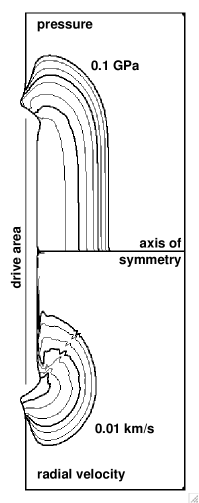
Figure 10: Spatially-resolved Lagrangian continuum dynamics simulation of edge release during ramp loading of Al. Loading was applied over a region 200 $\mu$m in diameter at the left side (shown by the grey line), ramping linearly to zero over 5 $\mu$m. The loading history was chosen to give a shock formation distance of 100 $\mu$m. The compression wave moves from left to right. The radius of the drive region was chosen to be equal to the shock formation distance, so that the scaled edge release distance is the fractional radius. This frame is at 9.8 ns after the start of loading, when the drive pressure has reached 50 GPa. Upper half shows pressure contours: 0.1, 0.2, 0.5, 1, 2, 5, 10, 20 GPa increasing from right to left. Lower half shows contours of the lateral (outward) component of particle velocity: 0.01, 0.02, 0.05, 0.1, 0.2, 0.5, 1 km/s. Exact powers of ten are thicker lines. The furthest advanced point is at the same radius as the edge of the drive region. In the drive region, edge release is approximately 55% of the way to the center, in agreement with the scaled edge release calculation. The simulations used a triangulated mesh with side lengths initially 2 $\mu$m.

V Example calculations for laser-driven material dynamics experiments

The applications and limitations of ramp loading using laser ablation depend on the type of laser used. We consider the following classes of laser:

High energy.

Laser systems delivering $o(100)$ J in a pulse. Currently-operating examples include TRIDENT at Los Alamos National Laboratory, JANUS at Lawrence Livermore National Laboratory, and OMEGA at the University of Rochester. These are relatively large, building-sized facilities, where experiments are performed at the facility. Previous experimental work has established these systems as recognized platforms for material dynamics studies, to a varying degree.

Medium energy.

Laser systems delivering $o(1)$ J,in a pulse. There are many such systems in existence. They are usually much smaller, fitting within a small room. It is often relatively straightforward to disassemble, crate, and re-assemble them, so it is feasible to transport them to other, fixed facilities which may provide a particular range of in-situ measurements such as diffraction from a synchrotron McNaney08 . However, the energy and pulse shaping is generally less suited to material dynamics experiments.

In the following sections we apply the ramp loading analysis to typical experimental configurations using these different classes of laser.

V.1 High energy lasers in nanosecond shock mode

Using JANUS and TRIDENT to generate shocks using ablation of nanosecond-scale pulses Swift_elements_04 , the minimum rise time of the laser pulse is around 0.1 ns. Pressures of interest in material dynamics studies are typically $\sim$10-100 GPa.

For a metal sample, loaded by direct ablation of the sample itself, the scaled rise time $\tau=0.05-0.15$ ns/$\mu$m, so 0.7-2 $\mu$m of the sample is subjected to a ramp before a shock forms. Samples are typically 10-200 $\mu$m thick, so they are largely shocked. A possible concern is diffraction from driven side if the x-ray penetration depth is not much greater than the shock formation distance.

If the sample is loaded by ablation of a plastic ablator, such as parylene Swift-chablator-07 , $\tau=0.2-0.3$ ns/$\mu$m, so 0.3-0.5 $\mu$m of the ablator is subjected to a ramp. This thickness is small compared with typical ablator thicknesses of 10-20 $\mu$m.

Edge release is not relevant during the shock formation stage: it affects a tiny region compared with typical laser spot sizes of 1-10 mm diameter.

V.2 High energy lasers in nanosecond ramp mode

The TRIDENT laser has been used previously to induce ramp loading with a shaped pulse up to 2.5 ns long Swift_lice_05 . For metal samples and a peak pressure of a few tens of gigapascals, a shock would form in 15-50 $\mu$m using the ideal loading history. The radial extent of the region affected by edge release would be 0.1-0.8 of this, which is small compared with typical TRIDENT drive spot diameters of 1-5 mm.

More recently, TRIDENT and JANUS have been modified to allow shaped pulses 10-20 ns long. For otherwise similar experiments, a shock would form in 60-400 $\mu$m. Care may be needed to control the extent of edge release when operating with a drive spot of diameter 1 mm or less.

V.3 High energy lasers in microsecond mode

The TRIDENT laser system can be operated in a frustrated amplification mode in which the pulse may be varied from around 50 ns to many microseconds. These long pulses may be used to ablate material confined by a transparent tamper Colvin07 ; Paisley08 ; Loomis07 . Pressures have been limited by breakdown of the tamper, and could likely be extended to higher pressures or longer durations by better spatial smoothing of the laser beam. Pressures of 10 GPa have been demonstrated, sustained for hundreds of nanoseconds. The pulse shape can be varied to induce shocks and ramps, among other shapes.

For shock loading, a Pockels cell has been used to clip the early part of the pulse, producing a minimum rise time of a few nanoseconds. The initial loading history is therefore a ramp, forming a shock in a thickness of around 100 $\mu$m.

Ramp loading has been demonstrated using a Gaussian pulse history of 160 ns full width, half maximum. Using the ideal loading history, a shock would form in $\sim$3 mm.

The edge release distance is around 0.2 of the shock formation distance, which is manageable for typical drive spot diameters of 5-8 mm.

Long pulses at TRIDENT have also been used to accelerate laser flyers for impact experiments Swift-flyer-05 . To minimize heating and damage in the flyer, the compression wave should preferably not induce a shock, so the shock formation distance should be greater than the flyer thickness. During the acceleration process, the ablation pressure typically reaches a maximum of around 0.1 GPa. Flyers have typically been 0.1-1 mm thick. The scaled rise time $\tau=5\times 10^{-4}$ ns/$\mu$m, implying a minimum rise time of 0.05-0.5 ns, which is far shorter than those generally used. The effects of edge release should be negligible for these pressures, so edge release of the ramp through the flyer thickness should not contribute significantly to curvature in the flyer.

V.4 Medium energy lasers

A portable loading laser has been used at the Advanced Photon Source synchrotron at Argonne National Laboratory to induce dynamic loading in samples with in-situ probing by synchrotron x-rays McNaney08 . The laser pulse had a Gaussian temporal profile of 12 ns full-width, half-maximum. The focal spot used to load the sample had a diameter of 250-300 $\mu$m. The laser pulse energy was around 0.4 J. Using a plastic ablator, the pressure induced in an Al sample should be in the range 1-10 GPa, implying a scaled rise time of $\tau=0.05-0.2$ ns/$\mu$m for shock formation. Thus a shock would form beyond a plastic thickness of 60-240 $\mu$m, which is thicker than typical for the ablator ($\sim$20 $\mu$m). In the sample itself, with or without an ablator, the scaled rise time is $\tau=0.01-0.05$ ns/$\mu$m, so a shock would form beyond a thickness of 240-1200 $\mu$m. This too is greater than the samples used, and thicker than a shock could be supported by that laser pulse length, so the drive was a ramp for all practical purposes.

The edge release region in typical ablators was much smaller than the drive spot. The edge release in typical samples ($\sim$100 $\mu$m thick) was also small.

VI Conclusions

We have derived expressions for ramp loading in compact, scaled form, allowing the adiabat for any material to be used to predict the distance for any arbitrary ramp to steepen into a shock. The calculation can be performed for adiabats expressed in tabular form, derived from material models of arbitrary complexity. The steepening relation can be used to determine the ‘ideal’ scaled loading history for a material, maximizing the distance for the shock to form. Steepening relations were derived for Al, Cu, and polyethene, as material representative of types commonly used in material dynamics studies. The propagation of lateral release waves across a ramp was analyzed, giving scaled relations for the region affected by lateral release when axial loading follows the ideal history. The analyses proceeded by considering characteristics; hydrocode simulations were used to verify the accuracy of the analyses.

The ramp evolution and edge release analyses were applied to situations in several types of laser loading experiment. It was demonstrated that properly-designed shock experiments at large-scale laser facilities do not subject unduly large amounts of the sample to ramp rather than shock loading from the finite rise time of the laser pulse, which has previously been a concern. The use of plastic ablators in particular eliminates any ramp region from the sample. The calculations also capture the limitations of ramp loading and the extent of lateral release in these experiments in a compact form, without requiring spatially-resolved simulations in two or even one dimension.

VII Acknowledgments

This work was performed in support of Laboratory-Directed Research and Development projects 06-SI-004 (Principal Investigator: Hector Lorenzana) and 08-ER-038 (Principal Investigators: Damian Swift and Bassem El-Dasher), under the auspices of the U.S. Department of Energy under contract DE-AC52-07NA27344.

References

- (1) For example, M.R. Boslough and J.R. Asay, in J.R. Asay, M. Shahinpoor (Eds), “High-Pressure Shock Compression of Solids” (Springer-Verlag, New York, 1992).
- (2) For example, C.A. Hall, J.R. Asay, M.D. Knudson, W.A. Stygar, R.B. Spielman, T.D. Pointon, D.B. Reisman, A. Toor, and R.C. Cauble, Rev. Sci. Instrum. 72, 3587 (2001).
- (3) D.C. Swift and R.P. Johnson, Phys. Rev. E 71, 066401 (2005).
- (4) D.C. Swift, T.E. Tierney IV, R.A. Kopp, and J.T. Gammel, Phys. Rev. E 69, 036406 (2004).
- (5) P. Peralta, D. Swift, E. Loomis, C.H. Lim, and K.J. McClellan, Metall. and Mat. Trans. A, 36, 6, 1459-1469 (2005).
- (6) J.M. McNaney, A. van Buuren, and H.E. Lorenzana, article in Advanced Photon Source experiments using a portable loading laser, in preparation.
- (7) D. Benson, Computer Methods in Appl. Mechanics and Eng. 99, 235 (1992).
- (8) D.C. Swift, Numerical solution of shock and ramp loading relations for general material properties, preprint arXiv:0704.0008 (2007).
- (9) J.P. Davis, C. Deeney, M.D. Knudson, R.W. Lemke, T.P. Pointon, and D.E. Bliss, Phys. Plasmas 12, 056310 (2005).
- (10) D.C. Swift, C.A. Forest, D.A. Clark, W.T. Buttler, M. Marr-Lyon, and P. Rightley, Rev. Sci. Instrum. 78, 6, 063904 (2007).
- (11) D.J. Steinberg, Equation of state and strength parameters for selected materials, Lawrence Livermore National Laboratory report UCRL-MA-106439 change 1 (1996).
- (12) D.C. Swift and R.G. Kraus, On the Properties of Plastic Ablators in Laser-Driven Material Dynamics Experiments, Phys. Rev. E (in press) and preprint arXiv:0712.1203 (2007).
- (13) Program and documentation for LAGC1D V6.0 (Wessex Scientific and Technical Services Ltd, Perth, 2007).
- (14) J.N. Fritz in S.C. Schmidt and W.C. Tau (eds), Shock Compression of Condensed Matter – 1995 (American Institute of Physics, Woodbury, 1995).
- (15) D.B. Hayes, C.A. Hall, J.R. Asay, and M.D. Knudson, J. Appl. Phys. 96, 10, pp 5520-5527 (2004).
- (16) L.M. Barker, in J.R. Asay, R.A. Graham, and G.K. Straub (Eds), Shock Waves in Condensed Matter – 1983, p. 17 (Elsevier, New York, 1984).
- (17) Program and documentation for EUL2D V0.6 (Wessex Scientific and Technical Services Ltd, Perth, 2007).
- (18) Program and documentation for LAGC V1.0 (Wessex Scientific and Technical Services Ltd, Perth, 2008).
- (19) J.D. Colvin, B.W. Reed, A.F. Jankowski, M. Kumar, D.L. Paisley, D.C. Swift, T.E. Tierney, and A.M. Frank, J. Appl. Phys. 101, 084906 (2007).
- (20) D.L. Paisley, S.-N. Luo, S.R. Greenfield, and A.C. Koskelo, Rev. Sci. Instrum. 79, 023902 (2008).
- (21) E. Loomis et al, theoretical study of confined ablation loading, in preparation.
- (22) D.C. Swift, J.G. Niemczura, D.L. Paisley, R.P. Johnson, S.-N. Luo, and T.E. Tierney, Rev. Sci. Instrum. 76, 093907 (2005).