The first $R_{cr}$ as a possible measure of the entrainment length in a 2D steady wake

Abstract

At a fixed distance from the body which creates the wake, entrainment is only seen to increase with the Reynolds number ($R$) up to a distance of almost 20 body scales. This increase levels up to a Reynolds number close to the critical value for the onset of the first instability. The entrainment is observed to be almost extinguished at a distance which is nearly the same for all the steady wakes within the $R$ range here considered, i.e. [20-100], which indicates that supercritical steady wakes have the same entrainment length as the subcritical ones. It is observed that this distance is equal to a number of body lengths that is equal to the value of the critical Reynolds number ($\sim 47$), as indicated by a large compilation of experimental results. A fortiori of these findings, we propose to interpret the unsteady bifurcation as a process that allows a smooth increase-redistribution of the entrainment along the wake according to the weight of the convection over the diffusion. The entrainment variation along the steady wake has been determined using a matched asymptotic expansion of the Navier-Stokes velocity field [Tordella and Belan, Physics of Fluids, 15(2003)] built on criteria that include the matching of the transversal velocity produced by the entrainment process.

Keywords: 2D steady wake, entrainment, critical Reynolds number, first instability

^♯ Dipartimento di Ingegneria Aeronautica e Spaziale, Politecnico di Torino, 10129 Torino, Italy

1 Introduction

The dynamics of entrainment and mixing is of considerable interest in engineering applications concerning pollutant dispersal or combustion, but it is also of great relevance in geophysical and atmospherical situations. In all these instances, flows tend to be complex. In most cases, entrainment is a time dependent multistage process in both the laminar and turbulent regime of motion.

The entrainment of external fluid in a shear flow such as that of a wake or a jet is a convective-diffusive process which is ubiquitous when the Reynolds number is greater than about a decade. It is a key phenomenon associated to the lateral momentum transport in flows which evolve about a main spatial direction. However, quantitative data concerning the spatial evolution of entrainment are not frequent in literature and are difficult to determine experimentally. Quantitative experimental observations are very cumbersome to obtain either in the laboratory or in the numerical simulation context. In some cases, such as, for instance, fluid entrainment by isolated vortex rings, theoretical studies (Maxworthy 1972[1]) predate experimental observations (Baird, Wairegi and Loo 1977[2]; Müller and Didden 1980[3]; Dabiri and Gharib 2004[4]).

It is interesting to note that more attention has been paid to complex unsteady and highly turbulent configurations in literature than to their fundamentally simpler steady counterparts.

In unsteady situations, entrainment is believed to consist of repeated cycles of viscous diffusion and circulatory transport. In turbulent flows, a sequence of processes is observed, where the exterior fluid is first ingested by the highly stretched and twisted interior turbulent motion (large-scale stirring) and is then mixed to the molecular level by the action of the small-scale velocity fluctuations, see for instance the recent experimental works carried out on free jets by Grinstein 2001[5] or on a plane turbulent wake by Kopp, Giralt and Keffer 2002[6].

In steady laminar shear flows, stretching dynamics is generally absent (as in 2D flows) or is close to its onset. In this case, entrainment is determined by the balance between the longitudinal and lateral nonlinear convective transport and the mainly lateral molecular diffusion.

Air entrainment in free-surface flows is another important instance of the entrainment process. The mechanism is complex and is also significant in nominally steady flows  e.g., a waterfall, or a steady jet. In such flows, entrainment is produced through the generation of cavities that can entrap air. The cavities are due to the impingement of the falling jet, which free-surface is usually strongly disturbed, over the liquid surface of the pool. As observed in Ohl, Oguz, Prosperetti 2000[7], the generation process takes advantage of both the kinetic energy of the jet surface disturbances and of part of the actual energy in the jet.

In this letter, we consider the steady two-dimensional (2D) wake flow past a circular cylinder. We deduce the entrainment as the longitudinal variation of the volume flow defect using a matched Navier-Stokes asymptotic solution determined in terms of inverse powers of the space variables (Belan and Tordella 2002[8]; Tordella and Belan 2003[9]), see Section 2. This approximated (2D) solution was obtained by recognizing the existence of a longitudinal intermediate region, which introduces the adoption of the thin shear layer hypothesis and supports a differentiation of the behaviour of the intermediate flow with respect to its infinite asymptotics. The streamwise behaviour of the entrainment is presented in Section 3. The concluding remarks are given in Section 4.

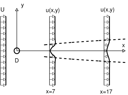
Figure 1: - Sketch of the physical problem. Longitudinal velocity profiles (solid lines) at $R=60$ and at stations $x=7$, $x=17$.

2 Analytical approximation of the velocity field, velocity flow rate defect and entrainment

For an incompressible, viscous flow behind a bluff body, the adimensional continuity and Navier-Stokes equations are expressed as

$$u\partial_{x}u+v\partial_{y}u+\partial_{x}p = R^{-1}\nabla^{2}u$$ (1)

$$u\partial_{x}v+v\partial_{y}v+\partial_{y}p = R^{-1}\nabla^{2}v$$ (2)

$$\partial_{x}u+\partial_{y}v = 0$$ (3)

where $(x,y)$ are the adimensional longitudinal and normal coordinates, $(u,v)$ the adimensional components of the velocity field, $p$ the pressure and $R$ the Reynolds number. The physical quantities involved in the adimensionalization are the length $D$ of the body that generates the wake, the density $\rho$ and the velocity $U$ of the free stream, see the flow schematic in fig. 1. The Reynolds number is defined as $R=\rho UD/\mu$, where $\mu$ is the dynamic viscosity of the fluid.

The velocity field for the intermediate region of the $2D$ steady wake behind a circular cylinder was obtained by matching an inner solution - a Navier-Stokes expansion in negative powers of the inverse of the longitudinal coordinate $x$

$$f_{i}= f_{i0}(\eta)+x^{-1/2}f_{i1}(\eta)+x^{-1}f_{i2}(\eta)+\cdots$$ (4)

where $f$ is a generic dependent variable and where the quasi-similar transformation $\eta=x^{-1/2}y$ is introduced, and an outer solution, which is a Navier-Stokes asymptotic expansion in powers of the inverse of the distance $r$ from the body

$$f_{o}=f_{o0}(s)+r^{-1/2}f_{o1}(s)+r^{-1}f_{o2}(s)+\cdots$$ (5)

where $r=\sqrt{x^{2}+y^{2}}$ and $s=y/x$.

The wake mass-flow deficit of the inner field was considered by means of an infield boundary condition carefully accounting for it. In fact, this condition is placed at the beginning of the intermediate flow region which inherits the full dynamics properties of near field. To this aim, we took advantage of experimental velocity and pressure profiles, as usually done in many physical contexts and as suggested, in the present context, by Stewartson (1957)[10]. Further details about the use of this infield condition are given below. It should be noted that the matched expansion in ranging from minus infinity to plus infinity in the transversal flow direction and that the concept of wake flow is clearly defined downstream from the intermediate region where the thin layer hypothesis starts to apply. The relevant boundary conditions involve, aside the infield condition, symmetry to the longitudinal coordinate and uniformity at infinity, both laterally and longitudinally. For details on the expansion term determination, the reader can refer to Tordella and Belan 2003[9].

The physical quantities involved in the matching criteria are the vorticity, the longitudinal pressure gradients generated by the flow and the transversal velocity produced by the mass entrainment process. The composite expansion is defined as $f_{c}=f_{i}+f_{o}-f_{common}$, where $f_{common}$ is the common part of the inner and outer expansions. In Tordella and Belan 2003[9] the explicit inner and outer velocity and pressure expansions can be found up to order four (i.e. $O(x^{-2})$ and $O(r^{-2})$, for the inner and outer wake, respectively), the composite approximation has been shown graphically. In this work, we approximate the wake flow with the composite solution obtained by truncating the inner and outer expansions at the third order term and then by determining their common part by taking the inner limit of the outer approximation. For the reader’s convenience, the inner and outer velocity component expansion terms are listed below (see equations 9 - 23). The common part has not been included because it has an analytical representation which alone would take up a few pages. However, the ©Mathematica file that describes its analytical structure and which allows its computation is given in the EPAPS online repository[11]. The common expansion was obtained by writing the inner and outer expansions in the primitive independent variables and by taking the inner limit of the outer expansion, that is, by taking the limit for $s\rightarrow 0$ and $r\rightarrow\infty$. To this end, the Laurent series of the outer expansion about $x\rightarrow\infty$ was considered up to the first order. The composite expansion - which is, by construction, a continuous curve, since it is obtained by the additive composition of three continuous curves, the sum of the inner and outer expansions minus the part they have in common - is accurate if the common expansion is accurate. This is always obtained if, at each order, the distance $\delta_{n}=|f_{i,n}-f_{o,n}|$ between the inner and the outer expansions is bounded and is at most of the same order as the range of $f_{i}$ and $f_{o}$. In the present matching, we have verified that in the matching region - that is, in the region where the composite connects the inner and the outer expansions - the distance $\delta_{n}$ is not only bounded, but is small with respect to the ranges of $f_{i}$ and $f_{o}$.

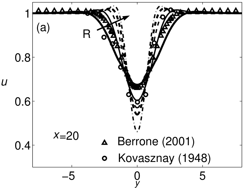
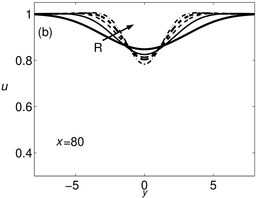
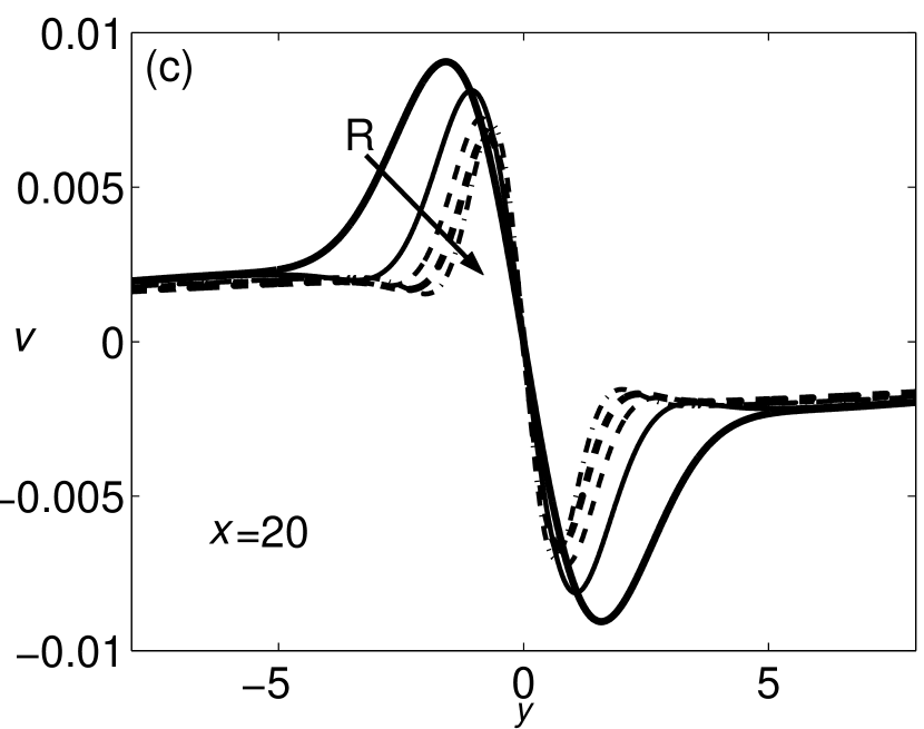
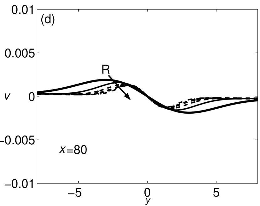
Figure 2: - Velocity profiles at the downstream stations $x=20$, $x=80$ and for $R=20,40,60,80$ and $100$. (a)-(b) Longitudinal velocity $u$, $x=20$ and $x=80$, (c)-(d) transversal velocity $v$, $x=20$ and $x=80$. The comparison with the numerical results by Berrone (2001) (triangles, $R=34$, $x=20$) and the laboratory data by Kovasznay (1948) (circles, $R=34$, $x=20$) is shown in part (a).

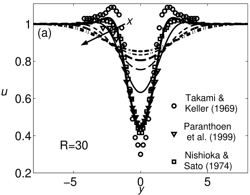
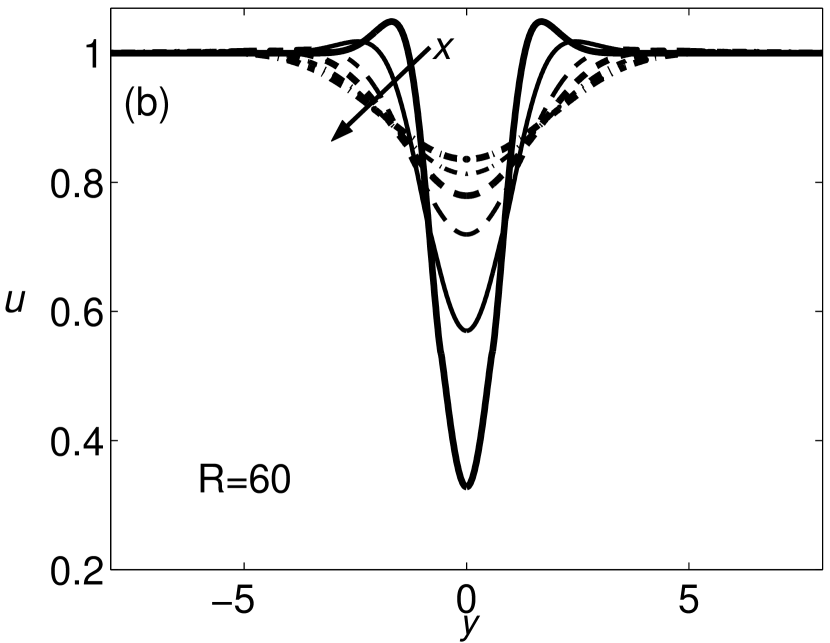
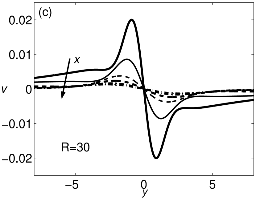
Figure 3: - Velocity profiles for $R=30,60$ plotted at stations $x=10,20,40,60,80$ and $100$. (a)-(b) Longitudinal velocity $u$, $R=30$ and $R=60$, (c)-(d) transversal velocity $v$, $R=30$ and $R=60$. The comparison with the experimental data by Nishioka & Sato (1974) (squares, $R=40$, $x=7$) and Paranthoen et al. (1999) (triangles, $R=34$, $x=10$) is shown in part (a).

The velocity approximation is shown in figures 2 and 3, where the longitudinal and transversal components of the composite solution for the velocity field are plotted for different longitudinal stations and Reynolds numbers.

It should be noted, that in this analytical flow representation, a few key properties of the wake flow have been taken into account. These properties can help an accurate description of the entrainment process to be obtained. These properties are:

i) The existence of intermediate asymptotics for the wake flow, in the general sense as given by Barenblatt and Zeldovich[12]. This is an important point, because the existence of the intermediate region supports the adoption of the thin shear layer hypothesis and relevant near-similar variable transformations for the inner flow, while, at the same time, it also supports a differentiation of the behavior of the intermediate flow with respect to its infinite asymptotics (Oseen’s flow).

ii) The use of an in-field boundary condition which consists of the distribution of the momentum and pressure at a given section along the mainstream of the flow in opposition to the use of integral field quantities. This kind of boundary condition is not new in literature[10], and presents the evident advantage of having a higher degree of field information with respect to the use of integral quantities such as the drag or the lift coefficients (a given integral value can be obtained from many different distributions).

iii) The acknowledgment of the fact that in free flows, such as low Reynolds numbers - 2D or axis-symmetric - wakes or jets developing in an otherwise homogeneous and infinite expanse of a fluid, the main role in shaping the flow is played by the inner flow. This directly inherits the main portion of the convective and diffusive transport of the vorticity, which is created, at the solid boundaries, by the motion of the fluid relative to the body. For these flows, it is physically opportune to denote the ”inner” flow as the straightforward or basic approximation. This means that, up to the first order, the inner solution is independent of the outer solution. According to this, the Navier-Stokes model, coupled with the thin layer hypothesis, very naturally yields the order of the field pressure variations $O(x^{-2})$. Pressure variations were often overestimated at $O(x^{-1})$[13],[9]. This was due to the use, in the inner expansion, of the assumption that the field can accommodate an inner pressure which is independent of the lateral coordinate, which however varies at the leading orders along the $x$ coordinate. However, at intermediate values of $y$ and for fixed $x$, this assumption is responsible for an anomalous rise in the composite expansion, due to the central plateau that appears in the outer expansion. The outer solution is in fact biased at finite values of $x$ to values greater than $1$ and forces the composite expansion to assume inaccurate values – with respect to experimental results – mostly in the region around $y/D\approx 2$ and outwards (at $y/D=20$ the longitudinal velocity is still appreciably different from $U$). For details, the reader may refer to Section IV and fig.6 in Tordella and Belan 2003[9].

iv) Last, we would like to point out that we have used the Navier-Stokes equations in the whole field, without the addition of any further restrictive axiomatic position, such as the principle of exponential decay. This did not prevent our approximated solution from spontaneously showing the properties of rapid decay and irrotationality at the first and second orders for the inner and the outer flows, respectively. At the higher orders, which mainly influence the intermediate region, the decay becomes a fast algebraic decay.

For an unitary spanwise length, the defect of the volumetric flow rate $D$ is defined as

$$D(x) = \int_{-\infty}^{+\infty}(1-u(x,y))dy$$ (6)

and is approximated through $u_{c}=u_{c}(x,y)$, the composite solution for the velocity field, as

$$D(x) \approx \int_{-\infty}^{+\infty}(1-u_{c}(x,y))dy.$$ (7)

Entrainment is the quantity that takes into account the variation of the volumetric flow rate in the streamwise direction, and is defined as

$$E(x)=|\displaystyle{\frac{dD(x)}{dx}}|.$$ (8)

The sequence of the first four terms of the inner and outer approximation for the streamwise velocity and the transversal velocity is given in the following.

Zero order, n=0,

$$u_{i0}(x,y) = c_{0}$$ (9)

$$v_{i0}(x,y) = 0$$ (10)

$$u_{o0}(x,y) = k_{0}$$ (11)

$$v_{o0}(x,y) = 0$$ (12)

with $c_{0}=1,k_{0}=1$.

First order, n=1

$$u_{i1}(x,y) = -Ac_{1}\textrm{e}^{-Ry^{2}/(4x)}x^{-1/2}$$ (13)

$$v_{i1}(x,y) = 0$$ (14)

$$u_{o1}(x,y) = 0$$ (15)

$$v_{o1}(x,y) = 0$$ (16)

with $c_{1}=1$, while the constant $A$ is related to the drag coefficient ($A=\textstyle{\frac{1}{4}}(R/\pi)^{1/2}c_{D}(R)$).

Second order, n=2

$$u_{i2}(x,y) = -\frac{1}{2}A^{2}\textrm{e}^{-Ry^{2}/(4x)}[\textrm{e}^{-Ry^{2}/(4x)}+\frac{1}{2}\frac{y}{\sqrt{x}}\sqrt{\pi R}\textrm{erf}(\frac{1}{2}\sqrt{\frac{R}{x}}y)]x^{-1}$$ (17)

$$v_{i2}(x,y) = -\frac{A}{2}\frac{y}{\sqrt{x}}\textrm{e}^{-Ry^{2}/(4x)}x^{-1}$$ (18)

$$u_{o2}(x,y) = 0$$ (19)

$$v_{o2}(x,y) = 0$$ (20)

Third order, n=3

$$u_{i3}(x,y) = A^{3}\textrm{e}^{-Ry^{2}/(4x)}(2-R\frac{y^{2}}{x})[\frac{1}{2}c_{3}-RF_{3}(x,y)]x^{-3/2}$$

$$v_{i3}(x,y) = -\frac{A^{2}}{2}\{-\frac{1}{2}\frac{y}{\sqrt{x}}\textrm{e}^{-Ry^{2}/(2x)}-\sqrt{\frac{\pi}{2R}}\textrm{erf}(\sqrt{\frac{R}{2x}}y)+(\frac{1}{2}\sqrt{\frac{\pi}{R}}+$$ (21)

$$- \frac{\sqrt{\pi R}}{4}\frac{y^{2}}{x})\textrm{e}^{-Ry^{2}/(4x)}\textrm{erf}(\frac{1}{2}\sqrt{\frac{R}{x}}y)\}x^{-3/2}$$

$$u_{o3}(x,y) = Re(\frac{i}{3}k_{31}e^{(3i/2)arctan(s)}+k_{33}\frac{s_{+}^{3/2}}{s^{3/2}}+\frac{1}{2}k_{32}s^{-3/2}s_{+}^{3/2}$$

$$\times \{\frac{\sqrt{(1+is)s}(\frac{3}{4}-\frac{i}{i+s})}{2(i+s)}+\frac{(-1)^{1/4}}{16\sqrt{2}}log[\frac{(\frac{i-1}{\sqrt{2}}+\sqrt{s})(\frac{i-1}{\sqrt{2}}-(1-i)\sqrt{1+is}+\sqrt{s})}{(\frac{1-i}{\sqrt{2}}+\sqrt{s})(\frac{1-i}{\sqrt{2}}+(1-i)\sqrt{1+is}+\sqrt{s})})$$

$$v_{o3}(x,y) = Re(e^{(3i/2)arctan(s)}[k_{31}+k_{32}s^{+}\frac{s+i}{3(s-i)^{2}}])$$

where $c_{3}=-2.26605+0.15752R-0.00265R^{2}+0.00001R^{3}$, $F_{3}$ is the third order of the function

$$F_{n}(x,y)=\frac{1}{\sqrt{x}}\int_{0}^{y}\frac{\textrm{e}^{R\zeta^{2}/(4x)}}{\textrm{Hr}_{n-1}^{2}(x,\zeta)G_{n}(x,\zeta)}d\zeta$$ (22)

$$G_{n}(x,y)=A^{-n}\frac{1}{\sqrt{x}}\int_{0}^{y}M_{n}(x,\zeta)\textrm{Hr}_{n-1}(x,\zeta)d\zeta$$ (23)

where $M_{n}(x,y)$ is the sum of the non homogeneous terms of the general ordinary differential equation for the inner solution coefficients ($\phi_{n}$), $n\geq 1$, obtained from the $x$ component of the Navier-Stokes equation[8]^,[9], and $\textrm{Hr}_{n-1}(x,y)=\textrm{H}_{n-1}(\displaystyle{\frac{1}{2}\sqrt{\frac{R}{x}}y})$, where $\textrm{H}_{n}$ are Hermite polynomials. In the outer terms, the variables $r,s,s^{\pm}$ are defined as $r=\sqrt{x^{2}+y^{2}}$, $s=y/x$, $s^{\pm}=(1+s^{2})^{\pm 1/2}$ and the relevant constants are $k_{31}=\pm\frac{1}{2}A^{2}/2\sqrt{\pi/(2R)}$, $k_{32}=3ik_{31}$, $k_{33}=0$.

3 Discussion of the results

Before describing the entrainment features we have observed, let us first discuss the asymptotic behaviour of the inner expansion in the lateral far field, since this aspect is important to determine the entrainment decay. At finite values of $x$, the inner streamwise velocity decays to zero as a Gaussian law for $n=1$ and as a power law of exponent $-2$ for $n=2$ and of exponent $-3$ for $n\geq 3$. The cross-stream inner velocity goes to zero for $n=0,1$ and to a constant value for $n\geq 2$. This allows $v$ to vanish as $x^{-3/2}$ for $x\rightarrow\infty$. When $x\rightarrow\infty$ this approximation coincides with the Gaussian representation given by the Oseen approximation. It can be concluded that, at Reynolds numbers as low as the first critical value and where the non-parallelism of the streamlines is not yet negligible, the division of the field into two basic parts - an inner vortical boundary layer flow and an outer potential flow - is spontaneously shown up to the second order of accuracy ($n=1$). At higher orders in the expansion, the vorticity is first convected and then diffused in the outer field. This is the dynamical context in which the entrainment process takes place.

In figures 2 (a) and 3 (a), the longitudinal velocity profiles are contrasted with the experimental data available for steady flows by Berrone[14], Paranthoen et al.(1999)[15], Nishioka & Sato (1974)[16] and Kovasznay (1948)[17]. The accuracy on the velocity distributions, between the analytical data and the laboratory ones is lower than 5%. This estimate was obtained by contrasting the longitudinal velocity distribution $u$ with the laboratory and numerical distributions, considered as the reference distribution. To this end, we computed the deviation $\Delta_{ref}={\|u-u_{ref}\|_{0,x}}/{\|1-u_{ref}\|_{0,x}}$. At $R=34$, a deviation $\simeq 4.5\%\;$ was obtained for the laboratory results by Kowasznay, where $x$ is the station at $20$ diameters from the center of the cylinder, see fig.2. As for the data by Berrone, we find a $\Delta_{ref}$ of about $1.7\%$. At $x\sim 10$ we have a comparison with Paranthoen et al. and Nishioka and Sato, that yields a deviation $\Delta_{ref}$ of about $2.5\%$ and $1.5\%$, respectively, see fig.3.

The entrainment is closely linked to the lateral and far field asymptotic behaviour. Since a numerical experiment cannot be over an unbounded domain of a flow, this approach is not suitable for the study of the field asymptotic behaviour and, as a consequence, entrainment (however, numerical simulations can yield very accurate representations of the near field, in particular of the standing eddy region). As far as entrainment is concerned, we then contrasted our analytical data with laboratory data. We tried to exploit all the results available in literature, obtaining a comparison with Paranthoen et al. (1999)[15] and Kovasznay (1948)[17] because these authors present a sequence of velocity profiles (mainly in supercritical flow configurations) that extend into the intermediate wake. The comparison was instead not feasible with the data by Nishioka and Sato (1974)[16] since they mainly measured the near wake (standing eddy region).

Figure 4 shows the volumetric flow rate defect $D=D(x;R)$ and the entrainment $E=E(x;R)$ obtained from the composite expansion. It can be observed that the volumetric defect flow rate slowly decreases with the distance from the body (fig.4 a). This decrease is faster at the beginning of the intermediate wake and at the higher Reynolds values. Considering a fixed position $x$ (fig.4 c), the flow defect decreases with the Reynolds number. Fig.4 (a) includes data from the laboratory experiments by Paranthoen et al. (1999, $R=53.3$) and Kovasznay (1948, $R=56$), both carried out at a slight supercritical $R$ (unsteady regime). The difference between their results in not small, but it should be recognized that the difficulties in measuring at small values of the Reynolds number are exceptionally high. By considering the arithmetic mean between these two sets of data, an increase of more than $50\%$ with regards to the values of the steady configuration, for $x<20$, is observed.

Parts (b, d) of fig.4 concern the entrainment, that is, the spatial rate of change of the wake velocity defect. The important points are: - the initial high variation at the beginning of the intermediate part of the wake, which increases with $R$, - the higher experimental mean value near $x=10$ ($2.45\;10{-2}$ against $6.5\;10^{-3}$), - for all the $R$, the exhaust of the entrainment at a distance of about $50$ body lengths, - the collection of experimentally determined values of the critical $R$ number that has a median value of $46.6$: a fact that relates the entrainment exhaust length - $EEL$ - to $R_{cr}$ with a simple scaling, such as $EEL\;\sim\;{\displaystyle R_{cr}^{\,n}}$ with $n=1$. In fig.4 (d), one can also observe that at a constant distance $x$ from the body, the entrainment stops growing beyond around $R_{cr}$.

Though the connection between the entrainment length and the instability cannot be direct: - the first can be deduced as an integral property of the steady fully non linear version of the motion equations, - the second from the linear theory of stability, which is conceived to highlight the role of the perturbation characteristics and not of the integral properties of the basic flow, these results could be a fortiori used to interpret the bifurcation to the unsteady flow condition at $R_{cr}$ as a process that allows the wake to tune the entrainment, and, possibly, to redistribute it on a larger wake portion, according to the actual $R$ value.

It can be noticed that the decay distance is of the same order of magnitude as $R_{cr}$ and this shows that the scaling used in recent stability analyses[19],[18] to represent the slow time and space wake evolution - $\tau=\varepsilon t$ and $\xi=\varepsilon x$, where $\varepsilon=\displaystyle{\frac{1}{R}\sim\frac{1}{R_{cr}}}$ - is linked to the exhaust of the entrainment process. In fact, one can say that the unit value of the slow time and spatial scales is reached where the entrainment nearly ends.

4 Conclusions

The entrainment is observed to be intense in the intermediate wake downstream from the separation region where the two-symmetric standing eddies are situated. Here, the dependence on the Reynolds number is clear. The entrainment grows six-fold when $R$ is increased from 20 to 100. The subsequent downstream evolution presents a continuous decrement of the entrainment. For all the $R$ here considered, it has been observed that this decrease is almost accomplished at a distance from the body of about $50$ diameters, which is a value that is close to the critical value $R_{cr}$ for the onset of the first instability and the subsequent set up of the unsteady regime (the median value in literature being $R_{cr}=46.6$). The establishment of the unsteady regime could be interpreted as a way of overcoming the limitation on the entrainment intensity and decay imposed by the steady regime. The observed decay length confirms the validity of the scaling that is often adopted in wake stability studies carried out using the spatial and temporal multitasking approach.

The authors would like to thank Marco Belan from the Politecnico di Milano for several helpful discussions.

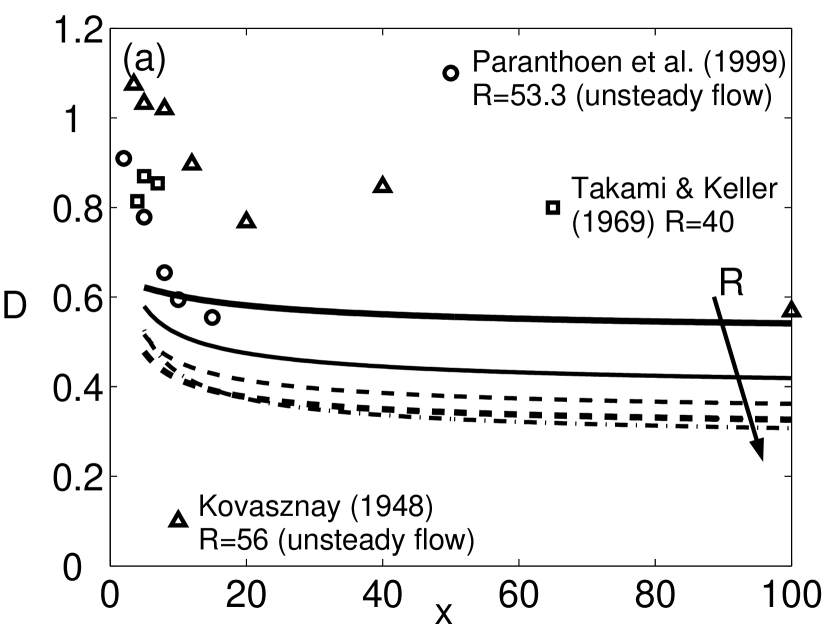
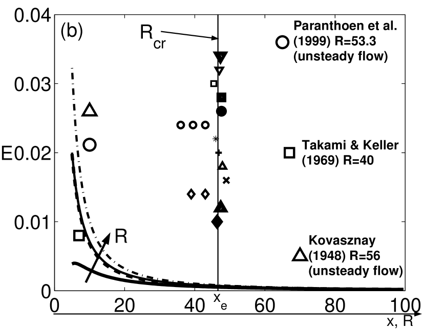
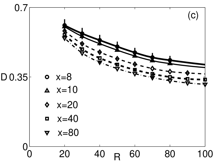
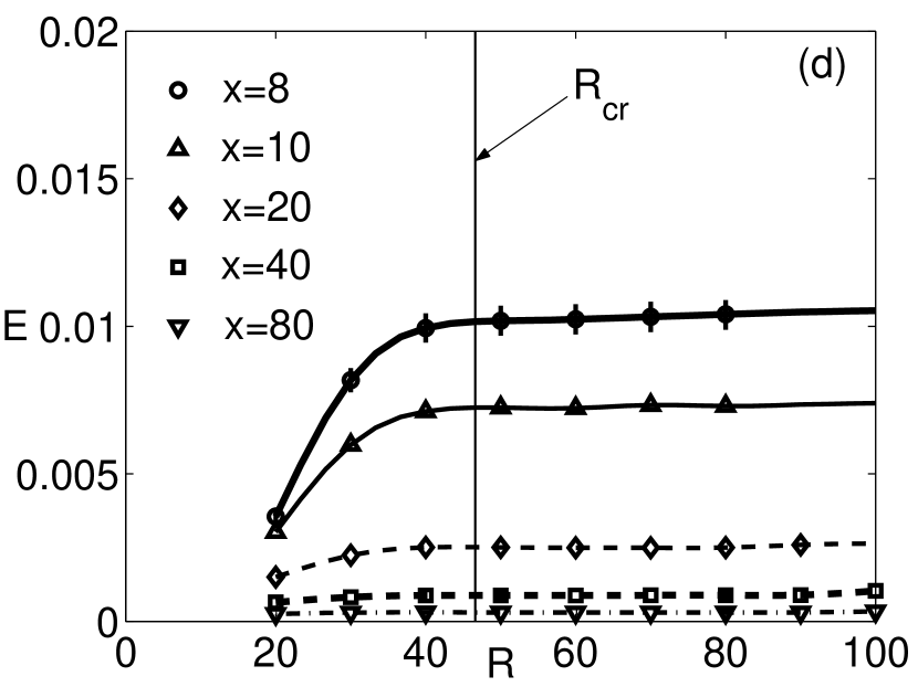
Figure 4: - (a)-(b): Downstream distribution of the volumetric flow rate defect $D$ and entrainment $E$ for $R=20,40,60,80$ and $100$. (c)-(d): Volumetric flow rate defect $D$ and entrainment $E$ as a function of the $R$ for different stations ($x=8,10,20,40,80$). The values of the volumetric flow rate defect $D$ for the oscillating (supercritical) wake, as inferred from experimental data by Kovasznay (1948, $R=56$) and Paranthoen et al. (1999, $R=53.3$), are also shown in part (a). The values of the critical Reynolds number obtained from different numerical and experimental results are placed at a distance from the body, $x_{e}$, equal to $R_{cr}$, see part (b). Position $x_{e}$ is observed to be the wake length where the entrainment is almost extinguished $\forall R\in[20,100]$, which leads to the hypothesis that the steady wake becomes unstable at a Reynolds number that is equal to the normalized distance where the entrainment almost ends and to the value beyond which the entrainment, at a constant distance from the body, stops growing (see part (d)). The symbols represent data from: Norberg 1994 ($\blacktriangle$), Zebib 1987 ($\lozenge$), Pier 2001 ($\times$), Williamson 1989 ($\vartriangle$), Leweke & Provansal 1995 ($+$), Strykowski & Sreenivasan 1990 ($\ast$), Coutanceau & Bouard 1977 ($\circ$), Elsenlhor & Eckelmann 1989 ($\bullet$), Hammache & Gharib 1989 ($\blacksquare$), Jackson 1987 ($\square$), Ding & Kawahara 1999 ($\blacklozenge$), Morzynski et al. 1999 ($\triangledown$), Kumar & Mittal 2006 ($\blacktriangledown$). The solid line in parts (b) and (d) indicates the median value ($R_{cr}\approx 46.6$) of these data.

References

- [1] Maxworthy, T. The structure and stability of vortex rings. J. Fluid Mech., 51: 15–32, 1972.
- [2] Baird, M. H. I., T. Wairegi and H. J. Loo. Velocity and momentum of vortex rings in relation to formation parameters. Can. J. Chem. Engng., 55: 19–26, 1977.
- [3] Müller, E. A. and N. Didden. Zur erzeugung der zirkulation bei der bildung eines ringwirbels an einer dusenmundung. Stroj. Casop., 31: 363–372, 1980.
- [4] Dabiri, J. O. and M. Gharib. Fluid entrainment by isolated vortex rings. J. Fluid Mech., 511: 311–331, 2004.
- [5] Grinstein, F. F. Vortex dynamics and entrainment in rectangular free jets. J. Fluid Mech., 437: 69–101, 2001.
- [6] Kopp, G. A., F. Giralt and J. F. Keffer. Entrainment vortices and interfacial intermittent turbulent bulges in a plane turbulent wake. J. Fluid Mech., 469: 49–70, 2002.
- [7] Ohl, C. D., H. N. Oguz and A. Prosperetti. Mechanism of air entrainment by a disturbed liquid jet. Physics of Fluids, 12 (7): 1710-1714, 2000.
- [8] Belan, M. and D. Tordella. Asymptotic expansions for two-dimensional symmetrical laminar wakes. ZAMM, 82 (4): 219–234, 2002.
- [9] Tordella, D. and M. Belan. A new matched asymptotic expansion for the intermediate and far flow behind a finite body. Physics of Fluids, 15 (7): 1897–1906, 2003.
- [10] Stewartson, K. On asymptotic expansions in the theory of boundary layers. J. Math. Phys., 36, 173, 1957.
- [11] ©Mathematica supplemental file: EPAPS-TS-WAKE-ENTRAINMENT.nb, online repository.
- [12] Barenblatt G.I., and Zel’dovich Y.B. Self-Similar Solutions as Intermediate Asymptotics. Annual Review of Fluid Mechanics, Vol. 4: 285-312 (Volume publication date January 1972) (doi:10.1146/annurev.fl.04.010172.001441)
- [13] Chang, I. Navier Stokes solutions at large distances from a finite body, J. Math. Mech., 10, 811, 1961.
- [14] Berrone, S. Adaptive discretizations of stationary and incompressible Navier-Stokes equations by stabilized Finite Element Methods. Comp. Methods in Appl. Mech. and Eng., 190/34: 4435–4455, 2001.
- [15] Paranthoen, P., L. W. B. Browne, S. Le Masson, F. Dumouchel and J. C. Lecordier. Characteristics of the near wake of a cylinder at low Reynolds Numbers. Eur. J. Mech. B/Fluids, 18: 659–674, 1999.
- [16] Nishioka, M. and H. Sato. Measurements of velocity distributions in the wake of a circular cylinder at low Reynolds numbers. J. Fluid Mech., 65, part 1, 97–112, 1974.
- [17] Kovásznay, L. S. G. Hot-wire investigation of the wake behind cylinders at low Reynolds numbers. Proc. Re. Soc. London S. A, 198: 174–190, 1948.
- [18] Tordella, D., S. Scarsoglio and M. Belan. A synthetic perturbative hypothesis for multiscale analysis of convective wake instability. Physics of Fluids, 18 (5), 2006.
- [19] Belan, M. and D. Tordella. Convective instability in wake intermediate asymptotics. J. Fluid Mech., 552: 127–136, 2006.
- [20] Norberg, C. An experimental investigation of the flow around a circular-cylinder - Influence of aspect ratio. J. Fluid Mech., 258: 287–316, 1994.
- [21] Zebib, A. Stability of viscous flow past a circular cylinder. J. Eng. Math., 21: 155–165, 1987.
- [22] Pier, B. On the frequency selection of finite-amplitude vortex shedding in the cylinder wake. J. Fluid Mech., 458: 407–417, 2002.
- [23] Williamson, C. H. K. Oblique and parallel modes of vortex shedding in the wake of a circular cylinder at low Reynolds numbers. J. Fluid Mech., 206: 579–627, 1989.
- [24] Leweke, T. and M. Provansal. The flow behind rings - Bluff-body wakes without end effects. J. Fluid Mech., 288: 265–310, 1995.
- [25] Strykowski, P. J. and K. R. Sreenivasan. On the formation and suppression of vortex shedding at low Reynolds-numbers. J. Fluid Mech., 218: 71–107, 1990.
- [26] Coutanceau, M. and R. Bouard. Experimental-determination of main features of viscous-flow in wake of a circular-cylinder in uniform translation. J. Fluid Mech., 79: 231–256, 1977.
- [27] Eisenlhor, H. and H. Eckelmann. Vortex splitting and its consequences in the vortex street wake of cylinders at low Reynolds-number. Physics of Fluids A-Fluid Dynamics, 1: 189–192, 1989.
- [28] Hammache, M. and M. Gharib. A novel method to promote parallel vortex shedding in the wake of circular-cylinders. Physics of Fluids A-Fluid Dynamics, 1: 1611–1614, 1989.
- [29] Jackson, C. P. A finite-element study of the onset of vortex shedding in flow past variously shaped bodies. J. Fluid Mech., 182: 23–45, 1987.
- [30] Ding, Y. and M. Kawahara. Three dimensional linear stability analysis of incompressible viscous flows using the finite element method. Int. J. Numer. Meth. Fluids, 31: 451 -479, 1999.
- [31] Morzynski, M., K. Afanasiev and F. Thiele. Solution of the eigenvalue problems resulting from global non-parallel flow stability analysis. Comput. Meth. Appl. Mech. Engrg., 169: 161 -176, 1999.
- [32] Kumar, B. and S. Mittal. Prediction of the critical Reynolds number for flow past a circular cylinder. Comput. Meth. Appl. Mech. Engrg., 195: 6046 -6058, 2006.