An exploratory analysis of the transient and long term behavior of small 3D perturbations in the circular cylinder wake

Abstract

An initial-value problem (IVP) for arbitrary small three-dimensional vorticity perturbations imposed on a free shear flow is considered. The viscous perturbation equations are then combined in terms of the vorticity and velocity, and are solved by means of a combined Laplace-Fourier transform in the plane normal to the basic flow. The perturbations can be uniform or damped along the mean flow direction. This treatment allows for a simplification of the governing equations such that it is possible to observe long transients, that can last hundreds time scales. This result would not be possible over an acceptable lapse of time by carrying out a direct numerical integration of the linearized Navier-Stokes equations. The exploration is done with respect to physical inputs as the angle of obliquity, the symmetry of the perturbation and the streamwise damping rate. The base flow is an intermediate section of the growing two-dimensional circular cylinder wake where the entrainment process is still active. Two Reynolds numbers of the order of the critical value for the onset of the first instability are considered. The early transient evolution offers very different scenarios for which we present a summary for particular cases. For example, for amplified perturbations, we have observed two kinds of transients, namely (1) a monotone amplification and (2) a sequence of growth - decrease - final growth. In the latter case, if the initial condition is an asymmetric oblique or longitudinal perturbation, the transient clearly shows an initial oscillatory time scale. That increases moving downstream, and is different from the asymptotic value. Two periodic temporal patterns are thus present in the system. Furthermore, the more a perturbation is longitudinally confined the more it is amplified in time. The long-term behavior of two-dimensional disturbances shows excellent agreement with a recent two-dimensional spatio-temporal multiscale modal analysis and with laboratory data concerning the frequency and wave length of the parallel vortex shedding in the cylinder wake.

Keywords: Initial-value problem (IVP) - perturbation - early transient - spatially developing flows -instability - absolute - periodic temporal patterns - growth - three-dimensional.

* corresponding author, e-mail: daniela.tordella@polito.it

^♯ Dipartimento di Ingegneria Aeronautica e Spaziale, Politecnico di Torino, 10129 Torino, Italy,

^♭ Department of Applied Mathematics, University of Washington, Seattle, WA 98195-2420, USA

1 Introduction

Recent shear flows studies ([1], [2], [3]) have shown the importance of the early time dynamics, that in principle can lead to non-linear growth long before an exponential mode is dominant. The recognition of the existence of an algebraic growth, due - among other reasons - to the non-orthogonality of the eigenfunctions ([4]) and a possible resonance between Orr-Sommerfeld and Squire solutions ([5]), recently promoted many contributions directed to study the early-period dynamics. For fully bounded flows works by [3], [6], [7], [8], [9], [10], and for partially bounded flows works by [11], [12], [13], [14] can be cited. As for free shear flows, the attention was first aimed in order to obtain closed-form solutions to the initial-value inviscid problem ([15], [16]) and was successful by considering piecewise linear parallel basic flow profiles.

An interesting aspect observed in the intermediate periods is that the maximal amplification is generally associated to oblique disturbances, that, as a consequence, potentially can promote early transition, see e.g. [13]. In fact, these perturbations, which are asymptotically stable at all Reynolds numbers, are the perturbations best exploiting the energy transient amplification.

In this work we consider as a prototype for free shear flow the two-dimensional wake past a bluff body. The wake stability has been widely studied by means of modal analyses (e.g. [17], [18], [19], [20]). However, in this way only the asymptotic fate can be determined, regardless of the transient behavior and the underlying physical cause of any instability.

In this work we adopt the velocity-vorticity formulation to evaluate the general initial-value perturbative problem. This method was proposed by Criminale, Drazin and co-authors in the years 1990-2000 ([2], [14], [16], [6], [11]). In synthesis, the variables are Laplace-Fourier transformed in the plane normal to the basic flow. Afterward, the resulting partial differential equations in time are integrated numerically. This procedure allows for completely arbitrary initial expansions by using a known set of functions (Schauder basis in the $L^{2}$ space) and yields the complete dynamics — the early time transients and the asymptotic behavior (up to many hundred time scales) — for any disturbance. The long term dynamics would not, in fact, have been easily recovered by using the alternative method of the direct numerical integration of the linear equations since the integration over a range of time larger than a few dozen basic time scales is not feasible.

The base flow model that we employ includes the wake transversal velocity and thus the nonlinear and diffusive dynamics that are responsible for the growth of the flow and the associated mass entrainment. We consider the first two order terms of the analytical Navier-Stokes expansion obtained by Tordella and Belan (2002, 2003) ([21], [22]), see §2.1. In particular, we consider the longitudinal component of such an expansion solution, the problem is parameterized by $x_{0}$, the longitudinal coordinate, and the Reynolds number $Re$.

We use a complex wavenumber for the disturbance component aligned with the flow so that longitudinal spatially damped waves are represented. It should be observed that a longitudinal spatial growth could not be considered physically admissible as an initial condition since the energy density of the initial perturbation would be infinite. In the context of the initial-value problem, this is an innovative feature adopted to introduce a possible spatial evolution (damping) of the perturbative wave in the longitudinal direction. The perturbative equations are numerically integrated by the method of lines. The equations formulation and initial and boundary conditions are presented in §2.2.

The perturbation evolution is examined for the base flow configurations corresponding to the Reynolds numbers of $50,100$, and for a typical section, $x_{0}=10$, of the intermediate region of the flow where the entrainment process is active. A comparison with a base flow far field configuration, $x_{0}=50$, is also proposed. The normalized perturbation kinetic energy density is the physical quantity on which the transient growth is observed (see §3.1). To determine the temporal asymptotics of the disturbance an equivalent of the modal temporal growth rate is introduced (see §3.3).

In the case of longitudinal disturbances, comparison with recent spatio-temporal multiscale Orr-Sommerfeld analysis ([23], [24]) and with laboratory experimental data ([27]) is carried out, see §3.3. As noted, the initial conditions posed are arbitrary. As far as the modal theory is concerned, the agreement is excellent both for the frequency, defined as the temporal derivative of the perturbation phase, and the temporal growth rate. It is also in quantitative agreement with respect to the laboratory data. The experiment shows couples of pulsation and wavelength of the cylinder vortex shedding that are close to those yielded by the IVP analysis when the wavenumber is that where the growth rate is maximum. Conclusions are given in §4.

2 Initial-value problem

2.1 Base flow

The base flow is considered viscous and incompressible. To describe the two-dimensional growing wake flow, an expansion solution for the Navier-Stokes two-dimensional steady bluff body wake ([22], [21]) has been used. The $x$ coordinate is parallel to the free stream velocity, the $y$ coordinate is normal. This approximated analytical Navier-Stokes solution incorporates the effects due to the full non linear convection as well as the streamwise and transverse diffusion. The solution was obtained by matching an inner Navier-Stokes expansion in terms of the inverse of the longitudinal coordinate $x$ ($x^{-n/2}$, $n=0,1,2,\ldots$) with an outer Navier-Stokes expansion in terms of the inverse of the distance from the body.

Here we take the first two orders ($n=0,1$) of the inner longitudinal component of the velocity field as a first approximation of the primary flow. In the present formulation the near-parallel hypothesis for the base flow, at a longitudinal position $x=x_{0}$, is made. The coordinate $x_{0}$ plays the role of parameter of the steady system together with the Reynolds number. The analytical expression for the profile of the longitudinal component is

$$\noindent U(y;x_{0},Re)=1-aC_{1}x_{0}^{-1/2}\rm e^{\displaystyle{-\frac{Re}{4}\frac{y^{2}}{x_{0}}}}$$ (1)

where $a$ is related to the drag coefficient ($a=\displaystyle{\frac{1}{4}}(Re/\pi)^{1/2}c_{D}(Re)$) and $C_{1}$ is an integration constant depending on the Reynolds number. As said in the introduction, this two terms representation is extracted from an analytical asymptotic expansion where the velocity vector and the pressure are determined to the forth order. It should be observed that the transversal velocity component $V$ first appears at the third order $(n=2)$, while the pressure only at the forth order $(n=3)$. Up to the second order, the field is thus parallel. Beyond the second order the analytical expression becomes much more complex, special functions as the confluent hypergeometric functions plays a role ([21]) associated to the deviation from parallelism. By changing the $x_{0}$ values, the base flow profile (1) will locally approximate the behavior of the actual wake generated by the body. Here, the region considered, if not otherwise specified, is fixed to a typical section, $x_{0}=10D$ (where $D$ is the spatial scale of the wake) of the intermediate wake. The term intermediate is used in the general sense as used by [28]: ’intermediate asymptotics are self-similar or near-similar solutions of general problems, valid for times, and distances from boundaries, large enough for the influence of the fine details of the initial/or boundary conditions to disappear, but small enough that the system is far from the ultimate equilibrium state…’. The distance beyond which the intermediate region is assumed to begin varies from eight to four diameters $D$ for $Re\in[20,40]$ (see [21], [22]). Base flow configurations corresponding to a $Re$ of $50,100$ are considered. In Figure 1 a representation of the wake profile at differing longitudinal stations is shown.

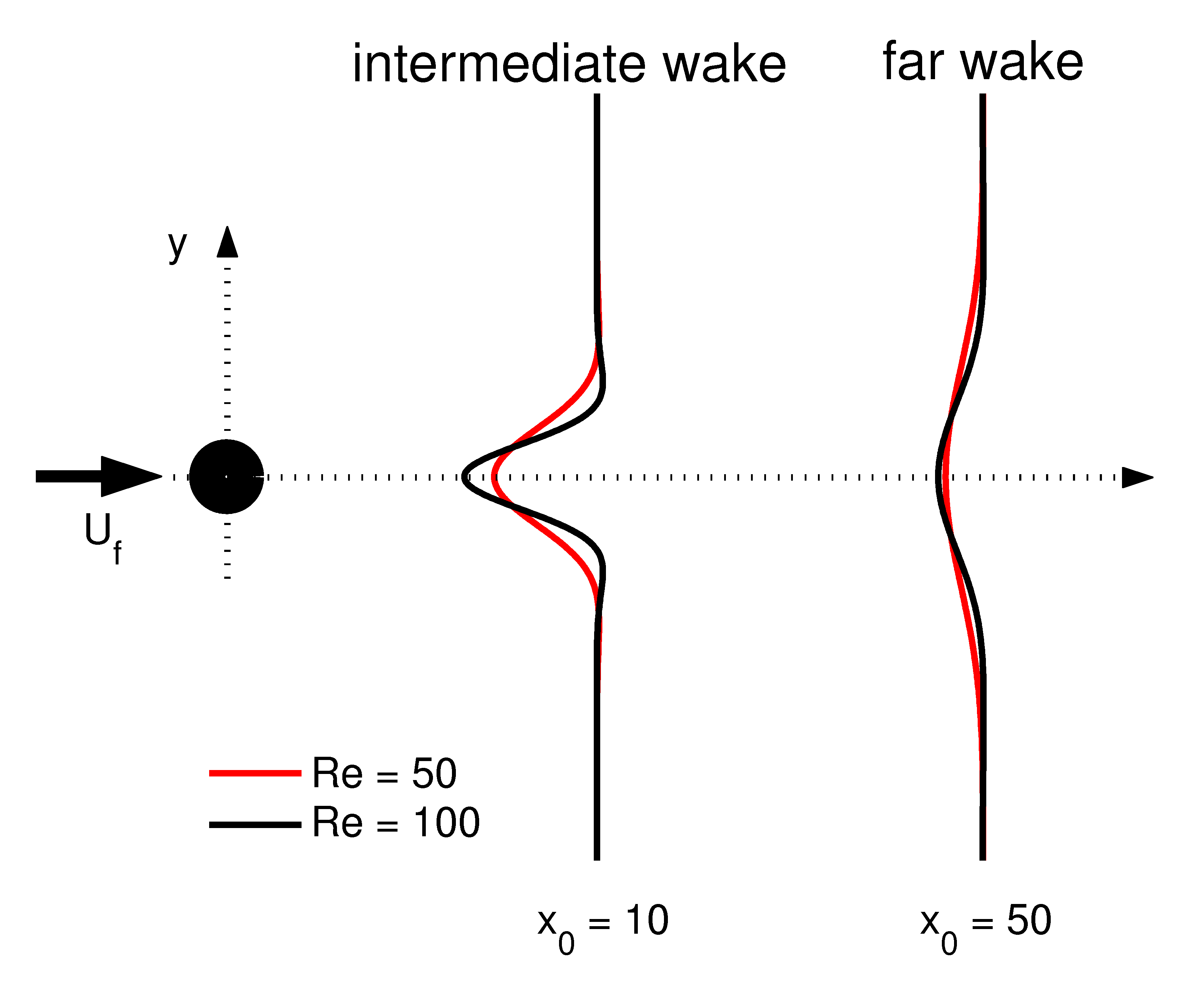
Figure 1: Wake schematic. Profile $U_{f}(y;x_{0},Re)$ in the intermediate ($x_{0}=10$) and far ($x_{0}=50$) wake for different Reynolds numbers, $U_{f}$ is the free stream velocity. The diameter of the cylinder is out of scale (three times) with respect to the wake profiles.

2.2 Formulation

By exciting the base flow with small arbitrary three-dimensional perturbations, the continuity and Navier-Stokes equations that describe the perturbed system are

$$\frac{\partial\widetilde{u}}{\partial x}+\frac{\partial\widetilde{v}}{\partial y}+\frac{\partial\widetilde{w}}{\partial z}=0$$ (2)

$$\frac{\partial\widetilde{u}}{\partial t}+U\frac{\partial\widetilde{u}}{\partial x}+\widetilde{v}\frac{\partial U}{\partial y}+\frac{\partial\widetilde{p}}{\partial x}=\frac{1}{Re}\nabla^{2}\widetilde{u}$$ (3)

$$\frac{\partial\widetilde{v}}{\partial t}+U\frac{\partial\widetilde{v}}{\partial x}+\frac{\partial\widetilde{p}}{\partial y}=\frac{1}{Re}\nabla^{2}\widetilde{v}$$ (4)

$$\frac{\partial\widetilde{w}}{\partial t}+U\frac{\partial\widetilde{w}}{\partial x}+\frac{\partial\widetilde{p}}{\partial z}=\frac{1}{Re}\nabla^{2}\widetilde{w}$$ (5)

where ($\widetilde{u}(x,y,z,t)$, $\widetilde{v}(x,y,z,t)$, $\widetilde{w}(x,y,z,t)$) and $\widetilde{p}(x,y,z,t)$ are the perturbation velocity components and pressure respectively. The independent spatial variables $z$ and $y$ are defined from $-\infty$ to $+\infty$, while $x$ is defined in the semispace occupied by the wake, from $0$ to $+\infty$. All physical quantities are normalized with respect to the free stream velocity $U_{f}$, the body scale $D$ and the density. By combining equations (3) to (5) to eliminate the pressure, the linearized equations describing the perturbation dynamics become

$$(\frac{\partial}{\partial t}+U\frac{\partial}{\partial x})\nabla^{2}\widetilde{v}-\frac{\partial\widetilde{v}}{\partial x}\frac{d^{2}U}{dy^{2}}=\frac{1}{Re}\nabla^{4}\widetilde{v}$$ (6)

$$(\frac{\partial}{\partial t}+U\frac{\partial}{\partial x})\widetilde{\omega}_{y}+\frac{\partial\widetilde{v}}{\partial z}\frac{dU}{dy}=\frac{1}{Re}\nabla^{2}\widetilde{\omega}_{y}$$ (7)

where $\widetilde{\omega}_{y}$ is the transversal component of the perturbation vorticity field. By introducing the quantity $\widetilde{\Gamma}$, that is defined by

$$\nabla^{2}\widetilde{v}=\widetilde{\Gamma}$$ (8)

we obtain three coupled equations (6), (7) and (8). Equations (6) and (7) are the Orr-Sommerfeld and Squire equations respectively, from the classical linear stability analysis for three-dimensional disturbances. From kinematics, the relation

$$\widetilde{\Gamma}=\frac{\partial\widetilde{\omega}_{z}}{\partial x}-\frac{\partial\widetilde{\omega}_{x}}{\partial z}$$ (9)

physically links together the perturbation vorticity components in the $x$ and $z$ directions ($\widetilde{\omega}_{x}$ and $\widetilde{\omega}_{z}$ respectively) and the perturbed velocity field. By combining equations (6) and (8) then

$$\frac{\partial\widetilde{\Gamma}}{\partial t}+U\frac{\partial\widetilde{\Gamma}}{\partial x}-\frac{\partial\widetilde{v}}{\partial x}\frac{d^{2}U}{dy^{2}}=\frac{1}{Re}\nabla^{2}\widetilde{\Gamma}$$ (10)

which, together with (7) and (8), fully describes the perturbed system in terms of vorticity. This formulation is a classical one. Alternative classical formulations, as the velocity-pressure one, are in common use. We chose this formulation because the vorticity transport and diffusion is the principal phenomenology for the dynamics of a wake system. For piecewise linear profiles for $U$ analytical solutions can be found. For continuous profiles, the governing perturbative equations cannot be analytically solved in general, but may assume a reduced form in the free shear case ([26]).

Moreover, from the equations (7), (8) and (10), it is clear that the interaction of the mean vorticity in $z$-direction ($\Omega_{z}=-dU/dy$) with the perturbation strain rates in $x$ and $z$ directions ($\frac{\partial\widetilde{v}}{\partial x}$ and $\frac{\partial\widetilde{v}}{\partial z}$ respectively) proves to be a major source of any perturbation vorticity production.

The perturbation quantities are Laplace and Fourier decomposed in the $x$ and $z$ directions, respectively. A complex wavenumber $\alpha=\alpha_{r}+i\alpha_{i}$ along the $x$ coordinate as well as a real wavenumber $\gamma$ along the $z$ coordinate are introduced. In order to have a finite perturbation kinetic energy, the imaginary part $\alpha_{i}$ of the complex longitudinal wavenumber can only assume non-negative values. In so doing, we allow for perturbative waves that can spatially decay ($\alpha_{i}>0$) or remain constant in amplitude ($\alpha_{i}=0$). The perturbation quantities $(\widetilde{v},\widetilde{\Gamma},\widetilde{\omega}_{y})$ involved in the system dynamics are now indicated as $(\hat{v},\hat{\Gamma},\hat{\omega}_{y})$, where

$$\hat{g}(y,t;\alpha,\gamma)=\int_{-\infty}^{+\infty}\int_{0}^{+\infty}\widetilde{g}(x,y,z,t)e^{-i\alpha x-i\gamma z}dxdz$$ (11)

indicates the Laplace-Fourier transform of a general dependent variable in the $\alpha-\gamma$ phase space and in the remaining independent variables $y$ and $t$. The governing partial differential equations are

$$\frac{\partial^{2}\hat{v}}{\partial y^{2}} - (k^{2}-\alpha_{i}^{2}+2ikcos(\phi)\alpha_{i})\hat{v}=\hat{\Gamma}$$ (12)

$$\frac{\partial\hat{\Gamma}}{\partial t}= - (ikcos(\phi)-\alpha_{i})U\hat{\Gamma}+(ikcos(\phi)-\alpha_{i})\frac{d^{2}U}{dy^{2}}\hat{v}$$ (13)

$$+ \frac{1}{Re}[\frac{\partial^{2}\hat{\Gamma}}{\partial y^{2}}-(k^{2}-\alpha_{i}^{2}+2ikcos(\phi)\alpha_{i})\hat{\Gamma}]$$

$$\frac{\partial\hat{\omega}_{y}}{\partial t}= - (ikcos(\phi)-\alpha_{i})U\hat{\omega}_{y}-iksin(\phi)\frac{dU}{dy}\hat{v}$$ (14)

$$+ \frac{1}{Re}[\frac{\partial^{2}\hat{\omega}_{y}}{\partial y^{2}}-(k^{2}-\alpha_{i}^{2}+2ikcos(\phi)\alpha_{i})\hat{\omega}_{y}]$$

where $\phi=tan^{-1}(\gamma/\alpha_{r})$ is the angle of obliquity with respect to the $x$-$y$ physical plane, $k=\sqrt{\alpha_{r}^{2}+\gamma^{2}}$ is the polar wavenumber and $\alpha_{r}=kcos(\phi)$, $\gamma=ksin(\phi)$ are the wavenumbers in $x$ and $z$ directions respectively. The imaginary part $\alpha_{i}$ of the complex longitudinal wavenumber represents the spatial damping rate in the streamwise direction. In figure 2 the three-dimensional perturbative geometry scheme is depicted.

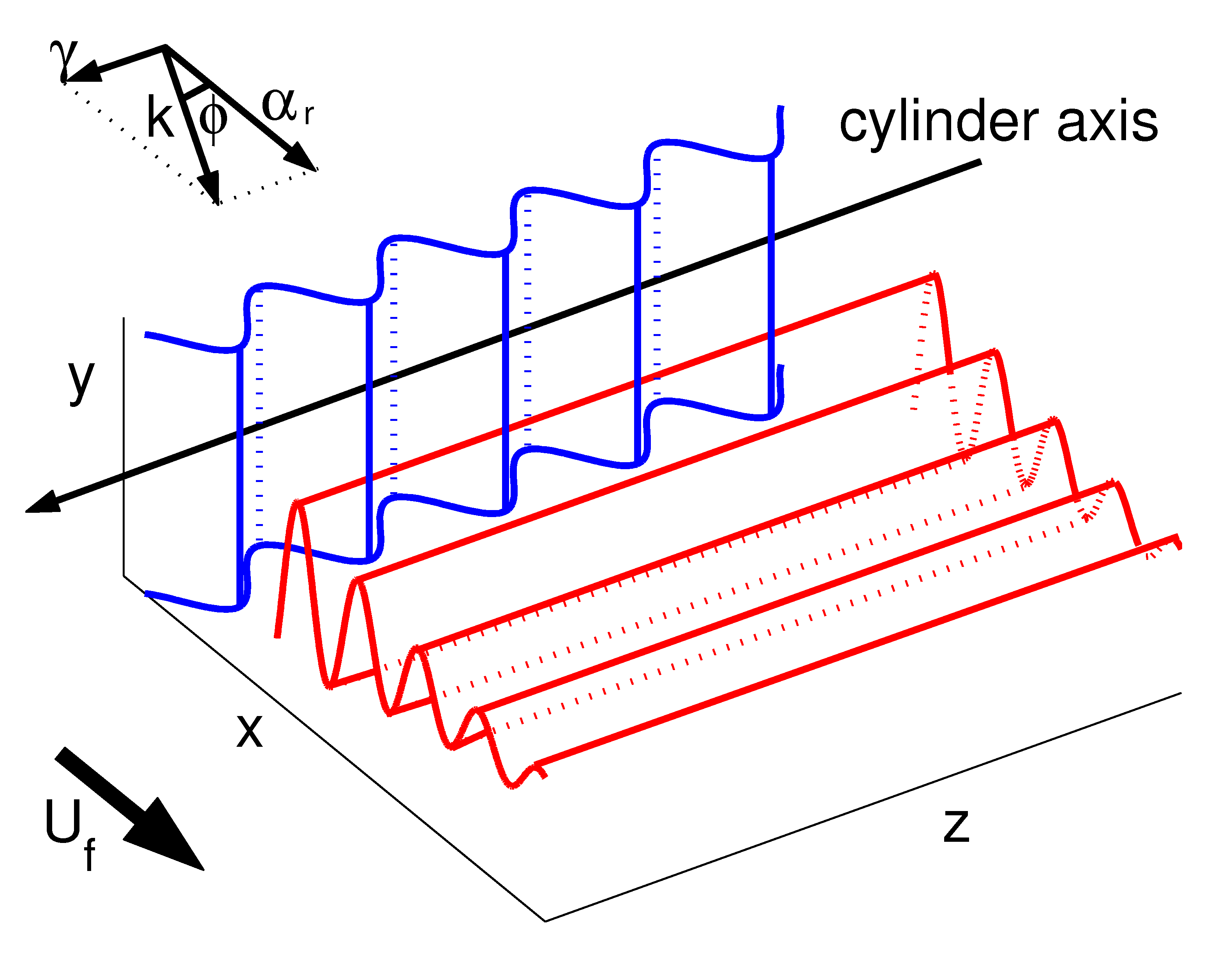
Figure 2: Perturbation geometry scheme.

From equations (12)-(14), it can be noted that there can neither be advection nor production of vorticity in the lateral free stream. The vorticity can only be diffused since only the diffusive terms remains in the limit when $y\rightarrow\infty$. Perturbation vorticity vanishes in the free stream, regardless if it is initially inserted there (if inserted, vorticity is finally dissipated in time when $y\rightarrow\infty$). This means that the velocity field is harmonic as $y\rightarrow\infty$.

Governing equations (12), (13) and (14) need proper initial and boundary conditions to be solved. Among all solutions, those whose perturbation velocity field is bounded in the free stream are sought. Periodic initial conditions for

$$\hat{\Gamma}=\frac{\partial^{2}\hat{v}}{\partial y^{2}}-(k^{2}-\alpha_{i}^{2}+2ikcos(\phi)\alpha_{i})\hat{v}$$ (15)

can be cast in terms of a set of functions in the $L^{2}$ Hilbert space, as

$$\hat{v}(0,y)=e^{-(y-y_{0})^{2}}\textmd{cos}(n_{0}(y-y_{0}))\,\,\,\,\textmd{or}\,\,\,\,\hat{v}(0,y)=e^{-(y-y_{0})^{2}}\textmd{sin}(n_{0}(y-y_{0})),$$

for the symmetric and the asymmetric perturbations, respectively. Parameter $n_{0}$ is an oscillatory parameter for the shape function, while $y_{0}$ is a parameter which controls the distribution of the perturbation along $y$ (by moving away, or bringing nearer, the perturbation maxima from the axis of the wake). The trigonometrical system is a Schauder basis in each space $L^{p}[0,1]$, for $1<p<\infty$. More specifically, the system $(1,sin(n_{0}y),cos(n_{0}y),\dots)$, where $n_{0}=1,2,\dots$, is the Schauder basis for the space of square-integrable periodic functions with period $2\pi$. This means that any element of the space $L^{2}$, where the dependent variables are defined, can be written as an infinite linear combination of the elements of the basis.

The transversal vorticity $\hat{\omega}_{y}$ is chosen initially equal to zero throughout the $y$ domain in order to ascertain which is the net contribution of three-dimensionality on the transversal vorticity generation and temporal evolution. However, it can be demonstrated that the eventual introduction of an initial transversal vorticity does not actually affect the perturbation temporal evolution.

Once initial and boundary conditions are properly set, the partial differential equations (12)-(14) are numerically solved by the method of lines. The spatial derivatives are centre differenced and the resulting system is then integrated in time by an adaptative multi-step method (variable order Adams-Bashforth-Moulton PECE solver). The transversal computational domain is large thirty body scales. By enlarging the computational domain to 50 and 100 body scales the results vary on the third and fourth significant digit, respectively.

2.3 Measure of the growth

One of the salient aspects of the initial-value problem is to observe the early transient evolution of various initial conditions. To this end, a measure of the perturbation growth can be defined through the disturbance kinetic energy density in the plane $(\alpha,\gamma)$ (see e.g [25],[26])

$$e(t;\alpha,\gamma,Re) = \frac{1}{2}\frac{1}{2y_{d}}\int_{-y_{d}}^{+y_{d}}(|\hat{u}|^{2}+|\hat{v}|^{2}+|\hat{w}|^{2})dy$$ (16)

$$= \frac{1}{2}\frac{1}{2y_{d}}\frac{1}{|\alpha^{2}+\gamma^{2}|}\int_{-y_{d}}^{+y_{d}}(|\frac{\partial\hat{v}}{\partial y}|^{2}+|\alpha^{2}+\gamma^{2}||\hat{v}|^{2}+|\hat{\omega}_{y}|^{2})dy,$$

where $2y_{d}$ is the extension of the spatial numerical domain. The value $y_{d}$ is defined so that the numerical solutions are insensitive to further extensions of the computational domain size. Here, we take $y_{d}=15$. The total kinetic energy can be obtained by integrating the energy density over all $\alpha_{r}$ and $\gamma$. The amplification factor $G(t)$ can be introduced in terms of the normalized energy density

$$G(t;\alpha,\gamma)=\frac{e(t;\alpha,\gamma)}{e(t=0;\alpha,\gamma)}.$$ (17)

This quantity can effectively measure the growth of a disturbance of wavenumbers $(\alpha,\gamma)$ at the time $t$, for a given initial condition at $t=0$ (Criminale et al. 1997; Lasseigne et al. 1999).

The temporal growth rate on the kinetic energy $r$

$$r(t;\alpha,\gamma)=\frac{log|e(t;\alpha,\gamma)|}{2t},\;\;\;t>0$$ (18)

is introduced in order to evaluate both the early transient as well as the asymptotic behavior of the perturbations (here it is the first moment of the perturbation which is assumed to asymptotically approach an exponential growth). Computations to evaluate the long time asymptotics are made by integrating the equations forward in time beyond the transient ([6], [11]) until the temporal growth rate $r$ asymptotes to a constant value ($dr/dt<\epsilon$, where $\epsilon$ is of the order $10^{-4}$). The angular frequency (pulsation) $\omega$ of the perturbation can be introduced by defining a local, in space and time, time phase $\varphi$ of the complex wave at a fixed transversal station (for example $y=1$) as

$$\hat{v}(y,t;\alpha,\gamma,Re)=A_{t}(y;\alpha,\gamma,Re)e^{i\varphi(t)}$$ (19)

and then computing the time derivative of the phase perturbation $\varphi$ ([29])

$$\omega(t)=\frac{d\varphi(t)}{dt}.$$ (20)

Since $\varphi$ is defined as the phase variation in time of the perturbative wave, it is reasonable to expect constant values of frequency, once the asymptotic state is reached.

3 Results

We present a summary of the most significant transient behavior and asymptotic fate of the three-dimensional perturbations. The temporal evolution is observed in the intermediate asymptotic region of the wake, which is the region where the spatial evolution is predominant. It can be demonstrated that changing the number of oscillations $n_{0}$ and the parameter $y_{0}$ that controls the perturbation distribution along the $y$ direction can only extend or shorten the duration of the transient, while the ultimate state is not altered. More specifically, if the perturbation oscillates rapidly or is concentrated mainly outside the shear region of the basic flow, for a stable configuration, the final damping is accelerated while, for an unstable configuration, the asymptotic growth is delayed. Thus, these two parameters are not crucial, because their influence can be recognized a priori. Therefore, in the following we use the two reference values, $n_{0}=1$ and $y_{0}=0$, and focus the attention mainly on parameters such as the obliquity, the symmetry, the value of the polar wavenumber and the spatial damping rate of the disturbance. In particular, the polar wavenumber $k$ changes in a range of values reaching at maximum the order of magnitude $O(1)$, according to what is suggested by recent modal analyses ([24], [23]). The order of magnitude of the spatial damping rate $\alpha_{i}$ varies around the polar wavenumber value.

3.1 Exploratory analysis of the transient dynamics

Figure 3 takes into account the influence, on the early time behavior, of the perturbation symmetry and of the wake region considered in the analysis, which is represented by the parameter $x_{0}$. All the configurations considered are asymptotically amplified, but the transients are different.

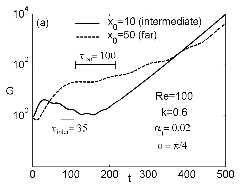
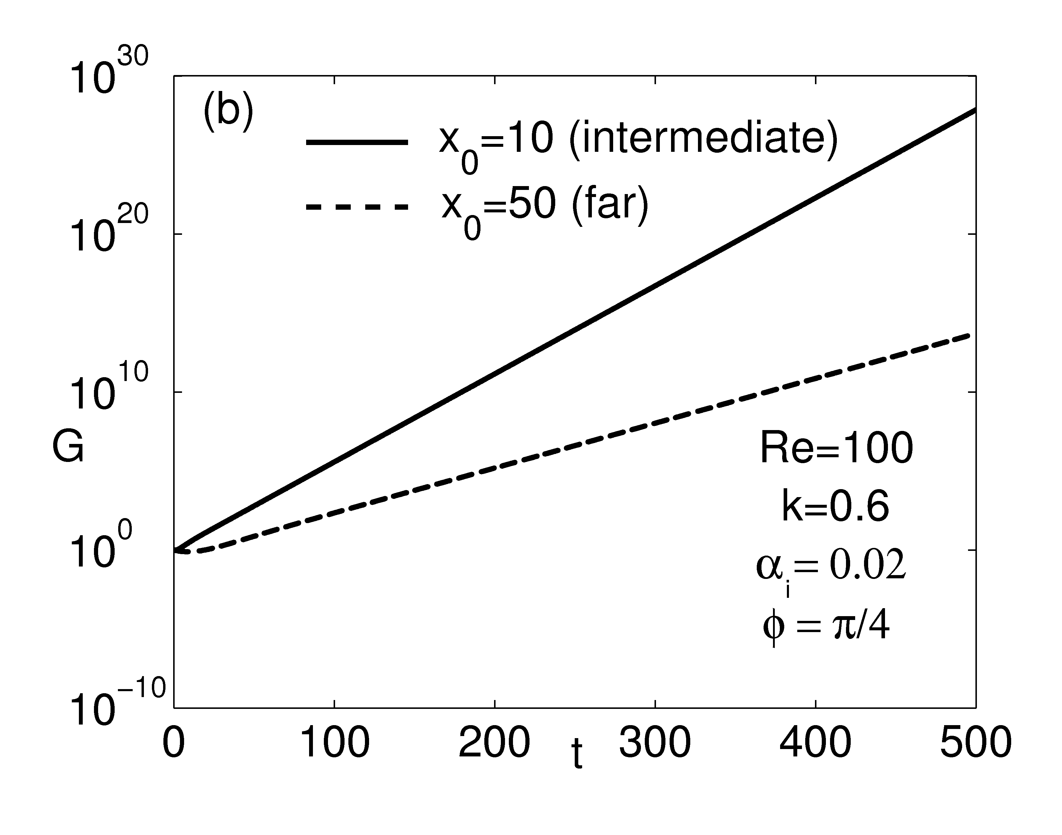
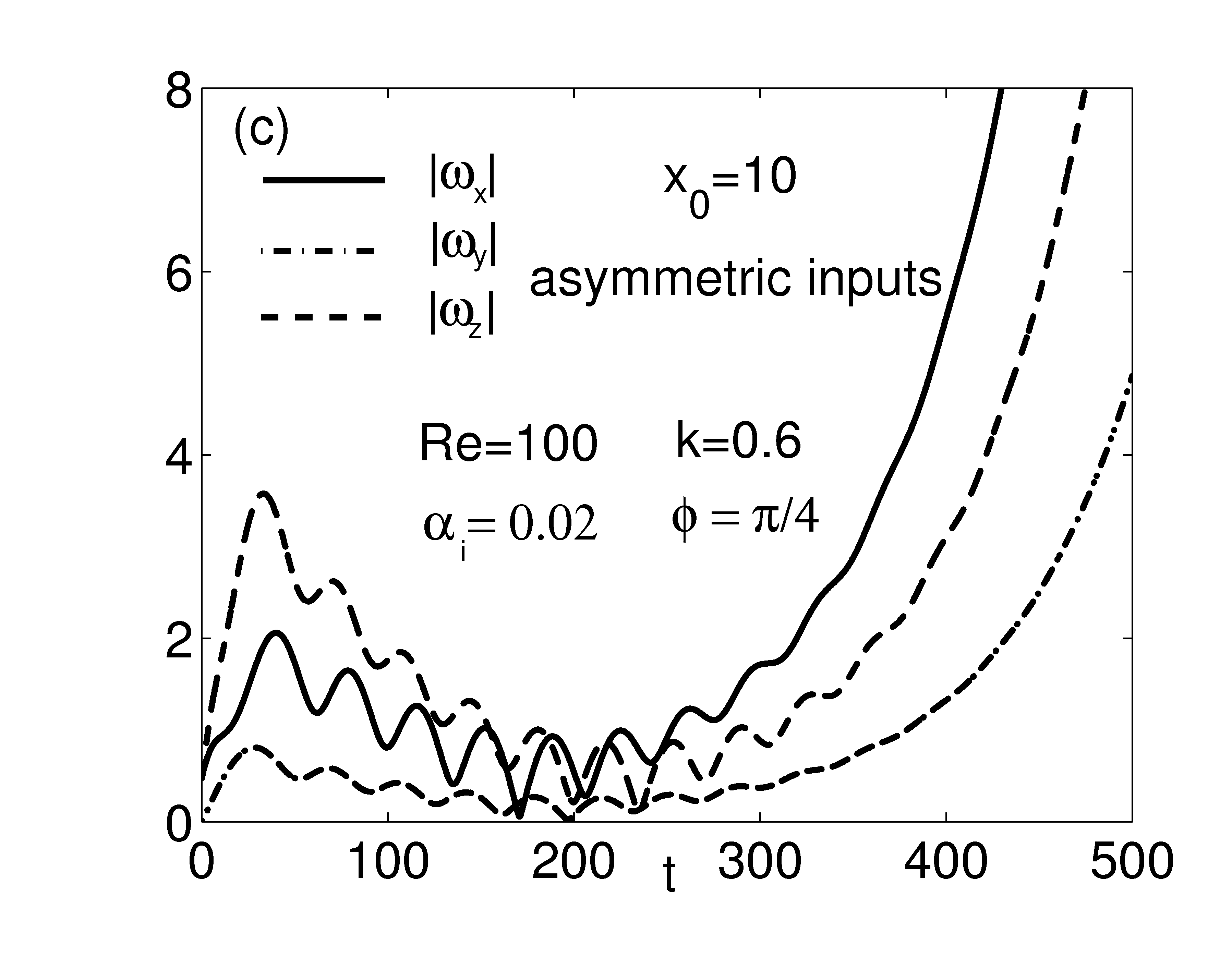
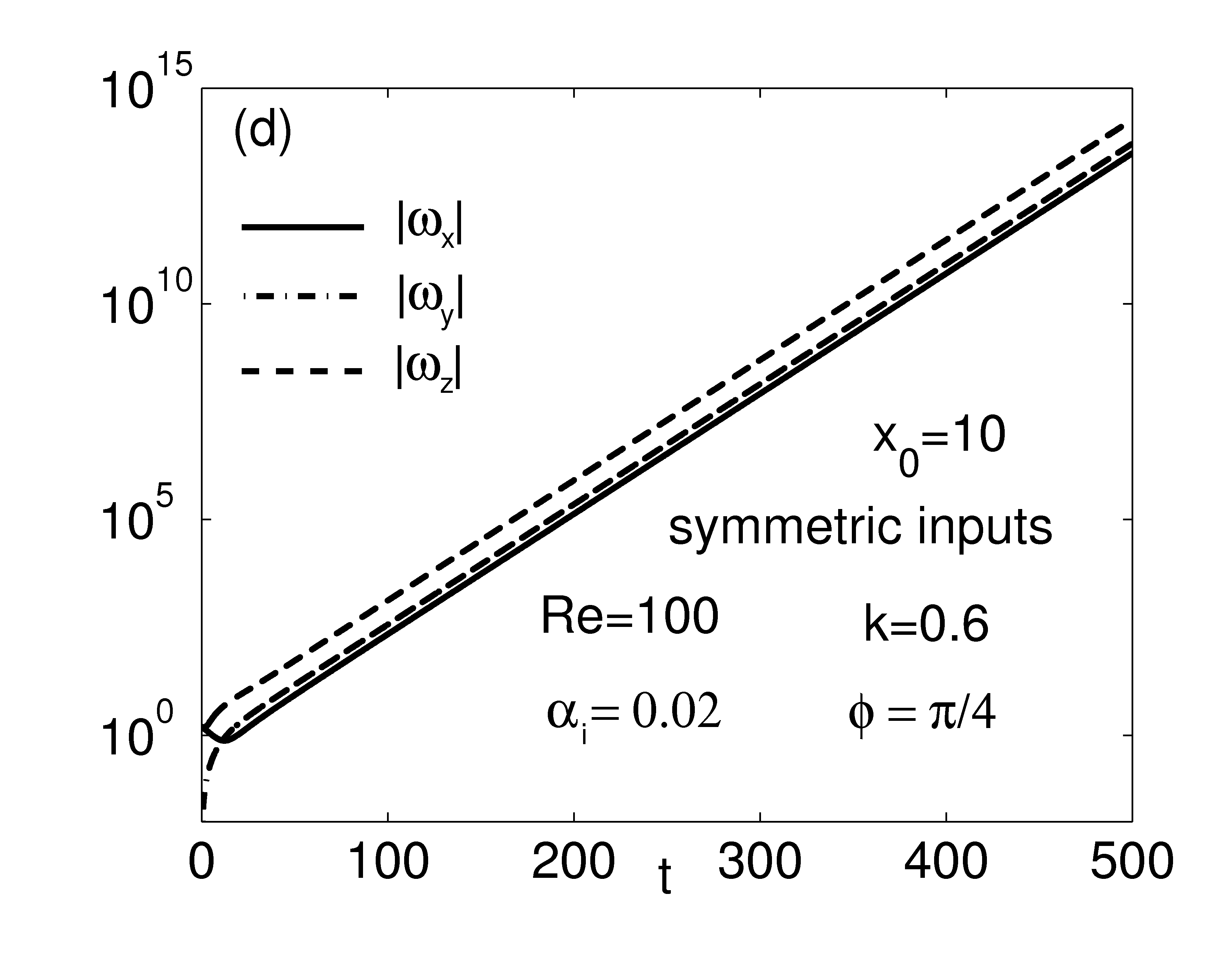
Figure 3: Effect of the symmetry of the perturbation. (a) - (b): The amplification factor $G$, and (c)-(d) the perturbation vorticity components at $y=1$ as a function of time. (a)-(c) asymmetric initial condition, (b)-(d) symmetric initial condition. Intermediate ($x_{0}=10$, solid curves) and far field ($x_{0}=50$, dashed curves) wake configurations. The periods $\tau_{inter},\tau_{far}$ are the periods of the modulation visible on $G$, in the intermediate and far field, respectively. The values of the vorticity component in part (d) have no physical meaning. The plot simply shows that, on the contrary of the asymmetric case in part(c), the symmetric disturbance growth has a short transient after which it becomes homogeneous in time.

The asymmetric cases (a) present, for both the intermediate position $x_{0}=10$ (solid curve) and the far field position $x_{0}=50$ (dashed curve), two temporal evolutions. For $x_{0}=10$ a local maximum, followed by a minimum, is visible in the energy density, then the perturbation is slowly amplifying and the transient can be considered extinguished only after hundreds of time scales. For $x_{0}=50$ these features are less marked. It can be noted that the far field configuration ($x_{0}=50$) has a faster growth than the intermediate field configuration ($x_{0}=10$) up to $t=400$. Beyond this instant the growth related to the intermediate configuration will prevail on that of the far field configuration. In the symmetric cases (b) the growths become monotone after few time scales ($t=20$) and the perturbations quickly reach their asymptotic states (around $t=50$). The intermediate field configuration ($x_{0}=10$, solid curve) is always growing faster than the far field configuration ($x_{0}=50$, dashed curve). This particular case shows a behavior that is generally observed in this analysis, that is, asymmetric conditions lead to transient evolutions that last longer than the corresponding symmetric ones, and demonstrates that the transient growth for a longitudinal station in the far wake can be faster than in the intermediate wake. It should be noted that, even if the asymmetric perturbation leads to a much slower transient growth than that observed for the symmetric case, the growth rate become equal when the asymptotic states are reached (see for example fig. 9). The temporal window shown in fig.3 ($t=500$) does not yet capture the asymptotic state of the asymmetric input. However, we observed that further in time the amplification factor $G$ reaches the same order of magnitude of the symmetric perturbation.

The more noticeable results presented in fig. 3 are that the asymmetric growths in the early transient are much less rapid than the symmetric ones and that the function $G$, in the case of asymmetric perturbations only, shows a modulation which is very evident in the first part of the transient, and which corresponds to a modulation in amplitude of the pulsation of the instability wave, see fig.4. In fact, the pulsation varies: in the early transient it oscillates around a mean value with a regular period, which is the same visible on G, and with an amplitude which is growing until this value jumps to a new value around which oscillates in a damped way. This second value is the asymptotic constant value. This behavior is always observed in the case of asymmetric longitudinal or oblique instability waves. Instead, it is not shown by transversal ($\phi=\pi/2$) waves or by symmetric waves, see fig. 4, where, on the one hand, the asymptotic value, nearly equal to that of the asymmetric perturbation, is rapidly reached after a short monotone growth and where, on the other, the growth is many orders of magnitude faster, and as a consequence, a modulation would not be easily observable. Thus, we may comment here on the fact that two time scales are observed in the transient and long term behavior of longitudinal and oblique perturbations: namely, the periodicity associated to the average value of the pulsation in the early transient, clearly visible in the asymmetric case only, and the final asymptotic pulsation. The asymptotic value of the pulsation is higher than the initial one, typically is about $2.5$ times higher. The period of the frequency modulation of the energy density $G$ is larger, nearly (1.4 - 1.7) higher, than the average period of the oscillating wave in the early transient, because $G$ is a square norm of the system solution. Thus the evolution of the system exhibits two periodic patterns at different frequencies: the first, of transient nature, and the other of asymptotic nature. When the average damping of the energy density in the early transient is not strong and is then followed by a monotone asymptotic growth, the change of the frequency of the oscillation is evident, see fig.4.

This kind of behavior is often observed in the study of linear systems with an oscillating norm, a problem that naturally arises in the context of the linearized formulation of convection-dominated systems over finite length domains. The occurrence of oscillating patterns in the energy evolution of the solutions is linked to the non-normal character of the linear operator which describes the system, see e.g. Coppola and De Luca (2006)[30].

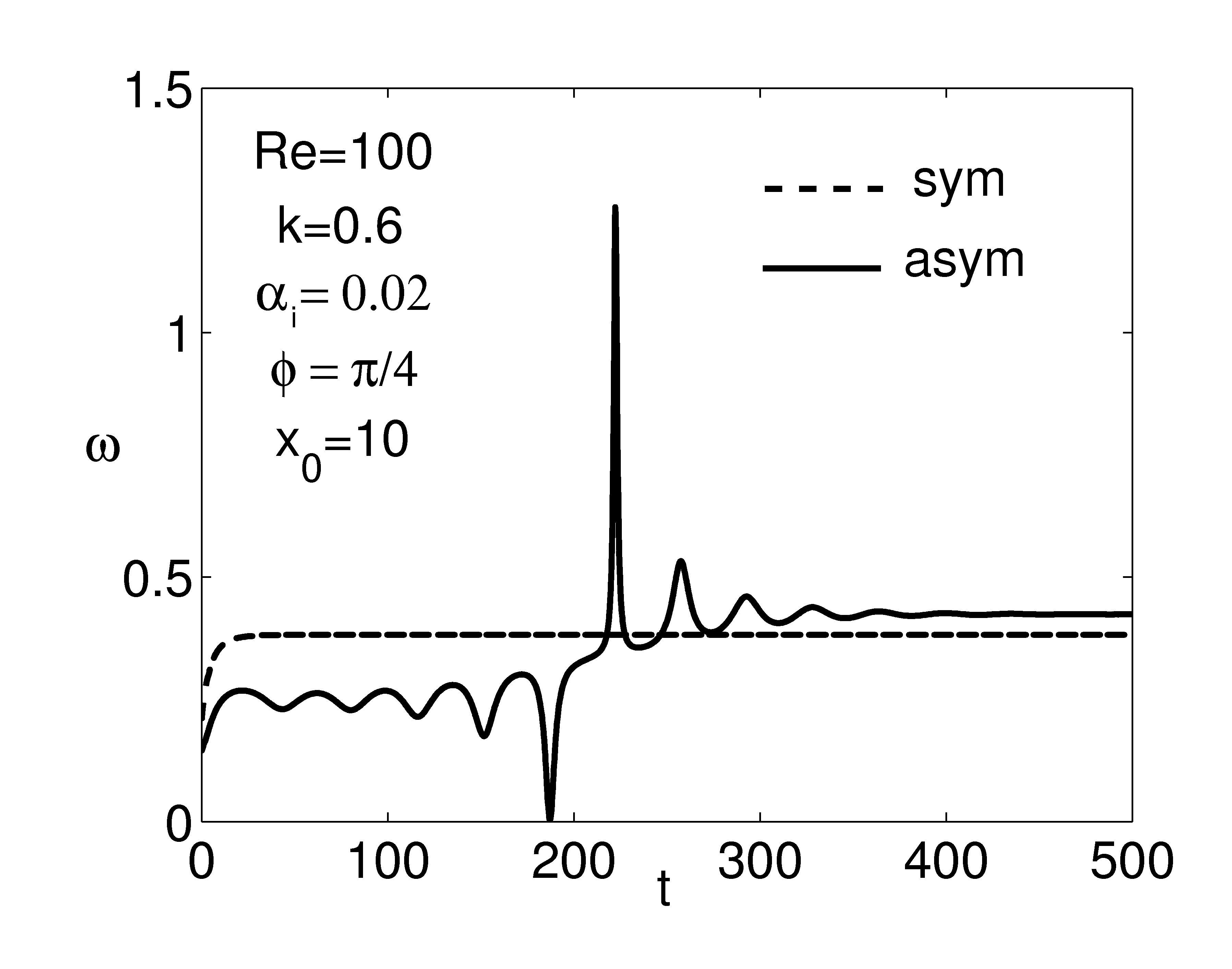
Figure 4: Pulsation behavior. The wave parameters are those shown in the previous figure, for $x_{0}=10$.

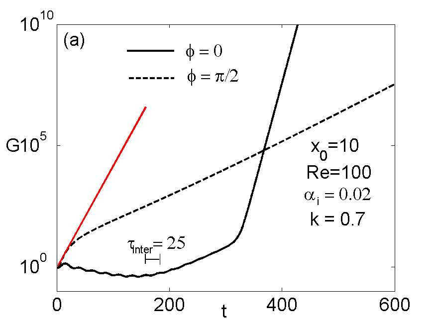
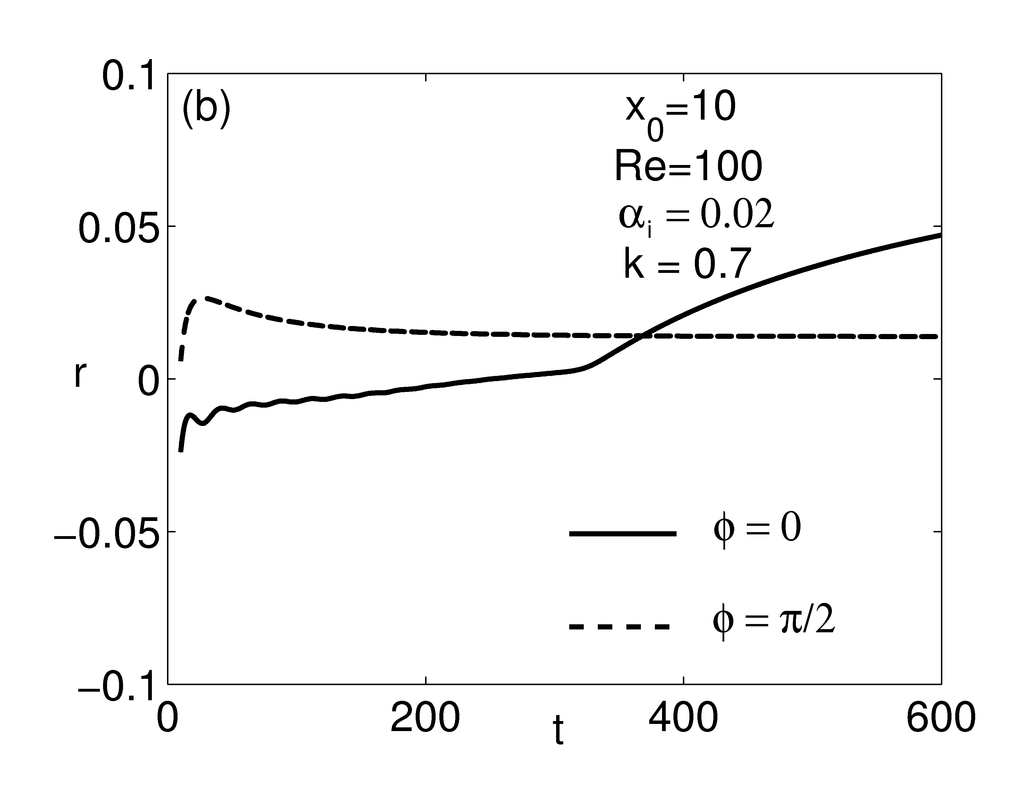
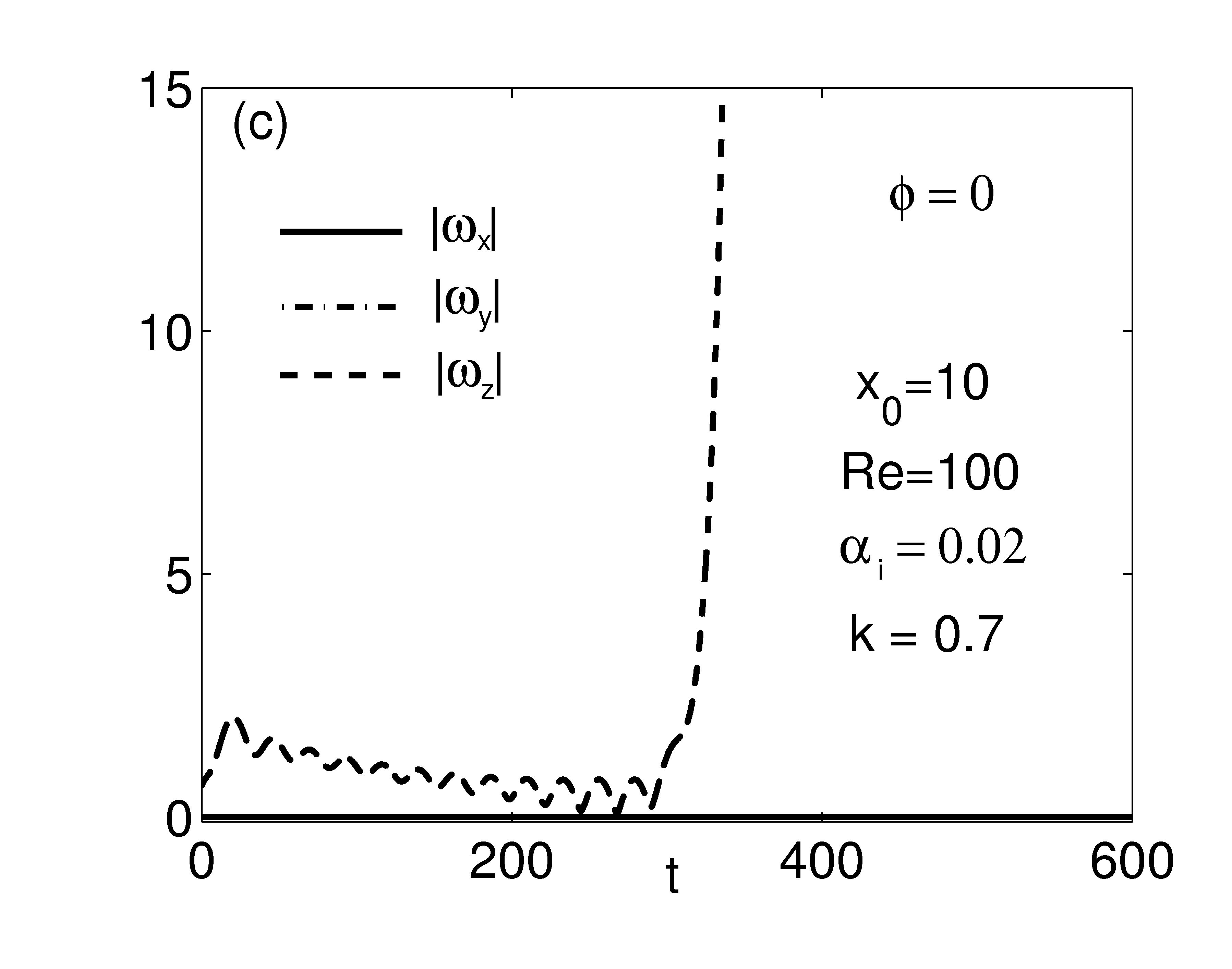
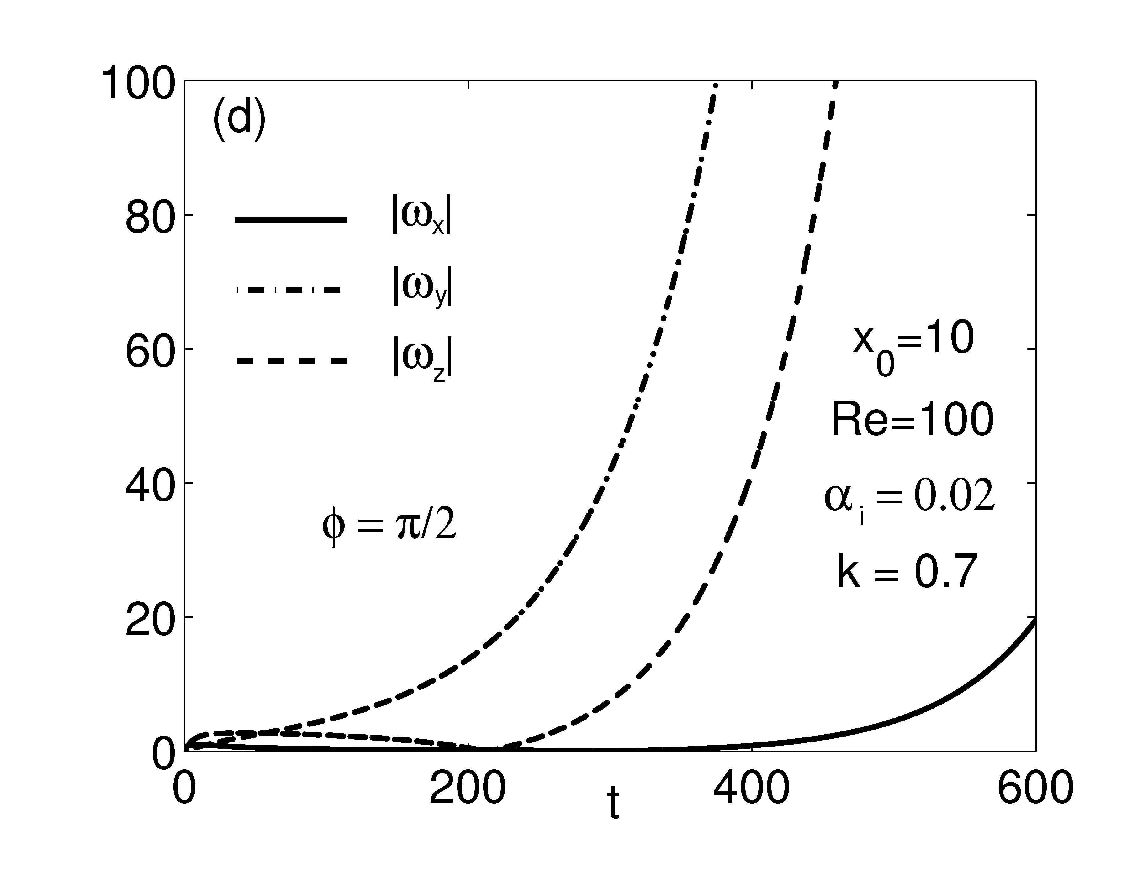
Figure 5: Effect of the angle of obliquity $\phi$. (a) The amplification factor $G$ and (b) the temporal growth rate $r$ as functions of time. Asymmetric initial condition, $\phi=0$ (solid curves), $\phi=\pi/2$ (dashed curves). (c)-(d) the perturbation vorticity components as functions of time at $y=1$, (c) $\phi=0$ and (d) $\phi=\pi/2$. The periods $\tau_{inter}$ is the period of the modulation visible on $G$, in the intermediate field.

Figure 5 illustrates an interesting comparison between two-dimensional and three-dimensional waves (note that a logarithmic scale on the ordinate is used in part (a) of Fig. 5). The purely two-dimensional wave (solid curve) is rapidly reaching a first maximum of amplitude (at about $t=15$), then the perturbation decreases while oscillating and reaches a minimum around $t=150$. Afterwards, the disturbance slowly grows up to $t\approx 300$, where an inflection point of the amplification factor $G$ occurs. It should be noted that this behavior is controlled solely by the evolution of the $\omega_{z}$, that is by the vorticity component present in the basic flow only. Then, the growth becomes faster and the perturbation is highly amplified in time. The purely orthogonal perturbation (dashed curve) is instead immediately amplified. The trend is monotone, and does not present visible fluctuations in time. The initial growth is actually rapid and an inflection point of the amplification factor $G$ can be found around $t=50$. Beyond this point, the growth changes its velocity and becomes slower, but still destabilizing. Both cases have asymmetric initial conditions and are ultimately amplified. In agreement with Squire theorem, the two-dimensional case turns out to be more unstable than the three-dimensional one, as the 2D asymptotically established exponential growth is more rapid than the 3D one (see solid and dashed curves in Fig. 5(a) for $t>400$). However, it should be noted that, for an extended part of the transient (up to about $t\approx 380$), the three-dimensional perturbation presents a larger growth than the two-dimensional one.

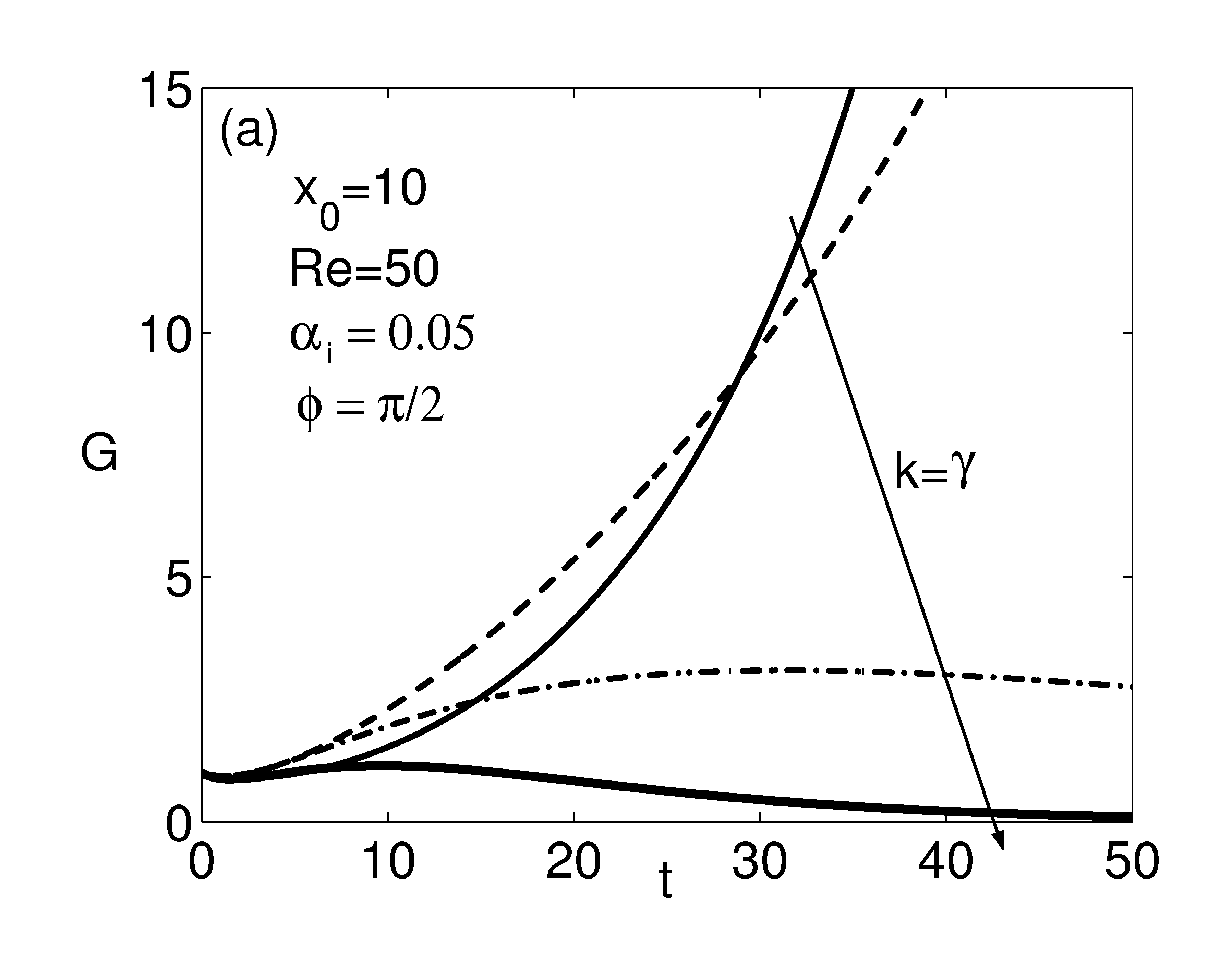
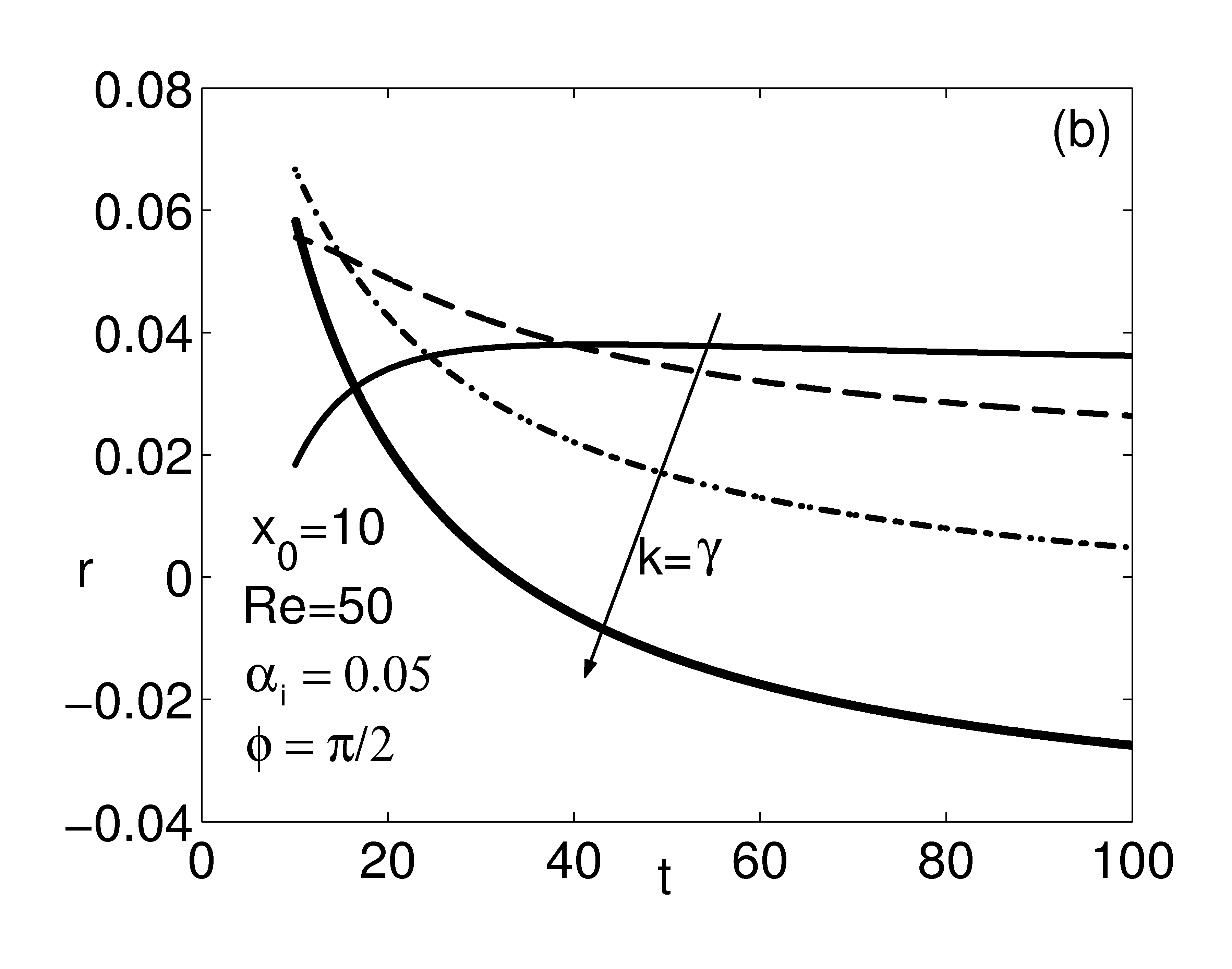
Figure 6: Effect of the polar wavenumber $k$. (a) The amplification factor $G$ and (b) the temporal growth rate $r$ as function of time. Symmetric initial condition, $k=0.5,1,1.5,2$.

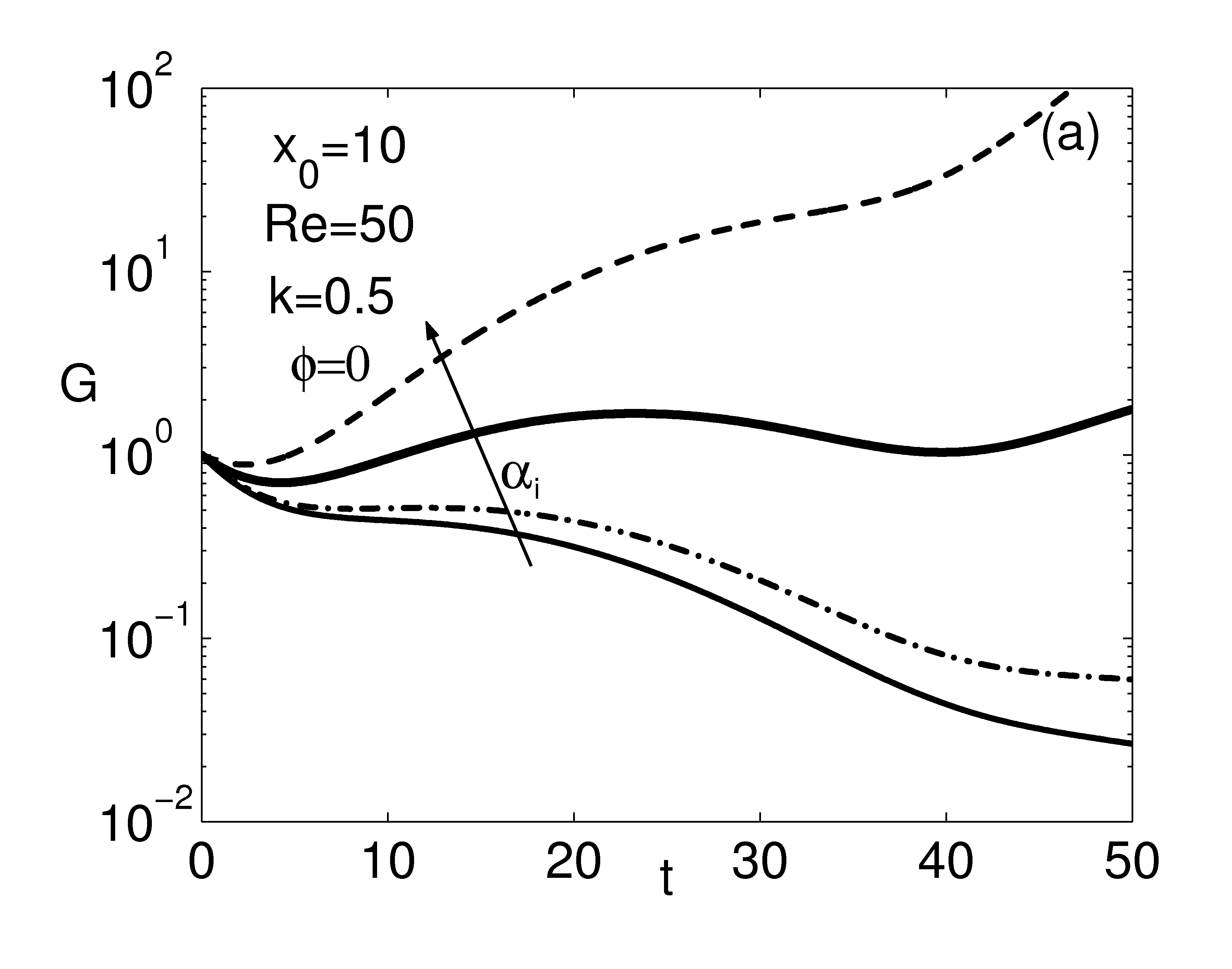
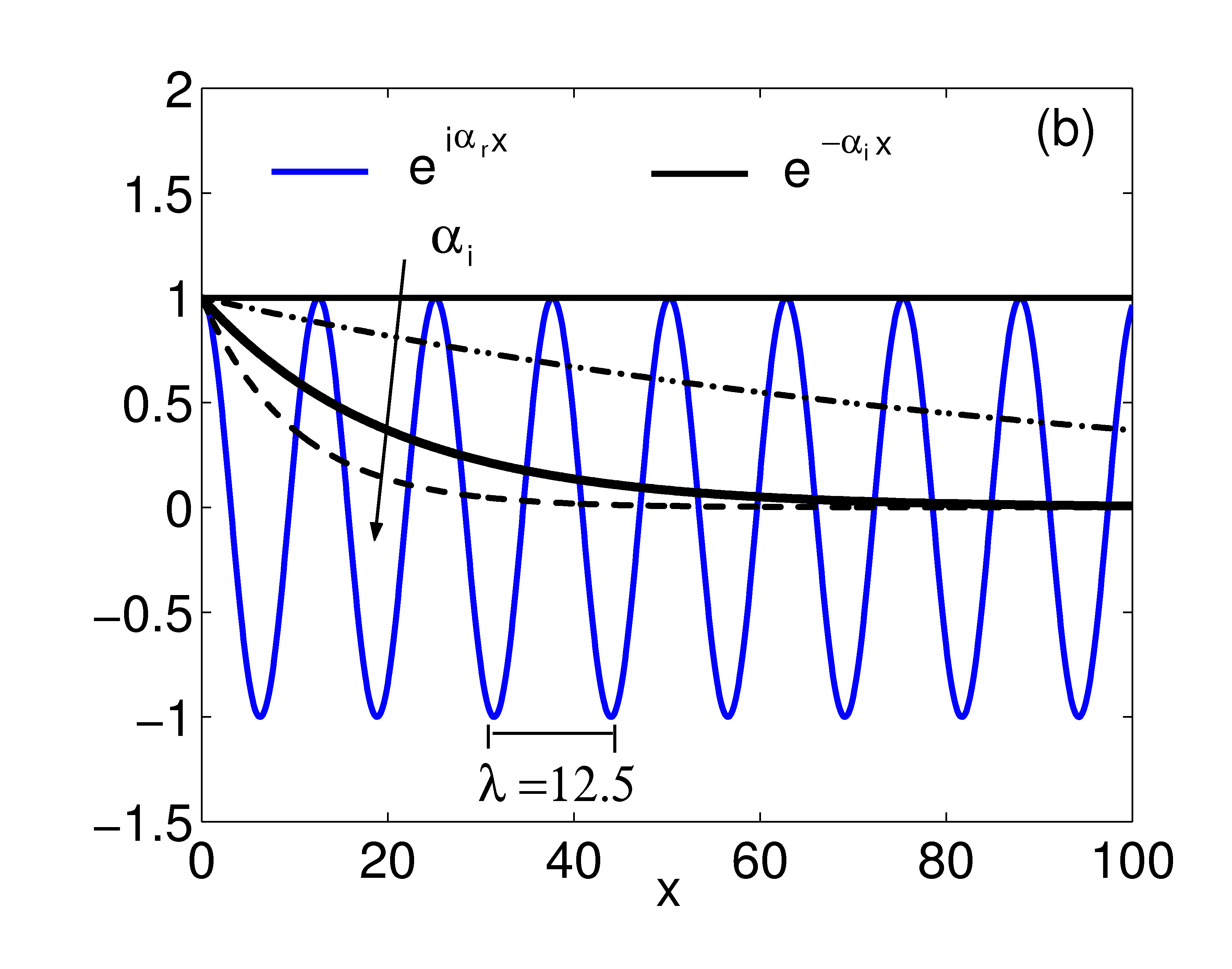
Figure 7: Effect of the spatial damping rate $\alpha_{i}$. (a) The amplification factor $G$ as function of time and (b) the wave spatial evolution in the $x$ direction for $k=\alpha_{r}=0.5$. Asymmetric initial condition, $\alpha_{i}=0,0.01,0.05,0.1$.

Fig. 6 demonstrates that purely orthogonal three-dimensional unstable perturbations may become damped by increasing their wavenumber ($k=\gamma$). In the case displayed in this figure, this happens when the wave number is increased beyond the value $1$. Before the asymptotic stable states are reached, these configurations yield maxima of the energy density (e.g. when $k=1.5,G\sim 3$ at $t\sim 30$) in the transients. This trend is also typical of oblique and longitudinal waves, and it can be considered a universal feature in the context of the stability of near parallel shear flows. It should be noted that, in fig. 6, the perturbation is symmetric and again the amplitude modulation is not observed in the early transient, even in the asymptotically stable situations. However, this example of transient behavior also contains a feature which is specific of orthogonal, both amplified or damped, and symmetric or asymmetric, perturbations, namely, the fact the most amplified component of the vorticity is the $\omega_{y}$, see also fig.5, part d.

In fig. 7 a significant phenomenon is observed for a longitudinal wave. By changing the order of magnitude of $\alpha_{i}$, it can be seen that perturbations that are more rapidly damped in space (see, in fig. 7b, the longitudinal spatial evolution of the wave) yield a faster growth in time. In fact, for nearly uniform waves in $x$ direction ($\alpha_{i}\rightarrow 0$) the configurations are asymptotically damped in time, while for increasing values of the spatial damping rate the perturbations are amplified in time (note that a logarithmic scale is used on part (a) of the figure). A possible general explanation is that the introduction in a physical system of a spatial concentration of kinetic energy is always destabilizing, hence the higher is the disturbance concentration the faster is the growth factor.

3.2 Physical interpretation of the different growth rate of symmetric and asymmetric disturbances

The dramatically increased growth rate of the symmetric mode with respect to the asymmetric mode can be understood from the induced velocity of the vorticity field. For simplicity, imagine that the wake consists of two parallel shear layers of opposite vorticity, as shown in figure 8(a). Further assume that the vorticity is discretized into a finite number of identical vortices. Suppose the upper shear layer is perturbed into a sinusoidal shape, as shown in figure 8(b). The induced velocity at the crest of the sinusoid at point 1 due to the other vortices in the upper shear layer alone is up and to the right as indicated by the arrow, corresponding to the classical Kelvin-Helmholtz instability.

Now consider the asymmetric mode, so that the lower shear layer is a sinusoid in phase with the upper one (figure 8(c)). The induced velocity at the crest of the lower shear layer at point 2 due to the other vortices in the lower shear layer alone is exactly the opposite of that at point 1. Thus the growth in the asymmetric mode is due to only higher order gradients in the induced velocity field of one shear layer on the other.

In contrast, with a symmetric perturbation, the lower shear is the mirror image of the upper. In figure 8(d), the induced velocity at point 2 is necessarily the mirror image of that at point 1. Both points move in concert to the right, without the low order velocity cancellation of the asymmetric mode. Thus the symmetric mode grows much faster.

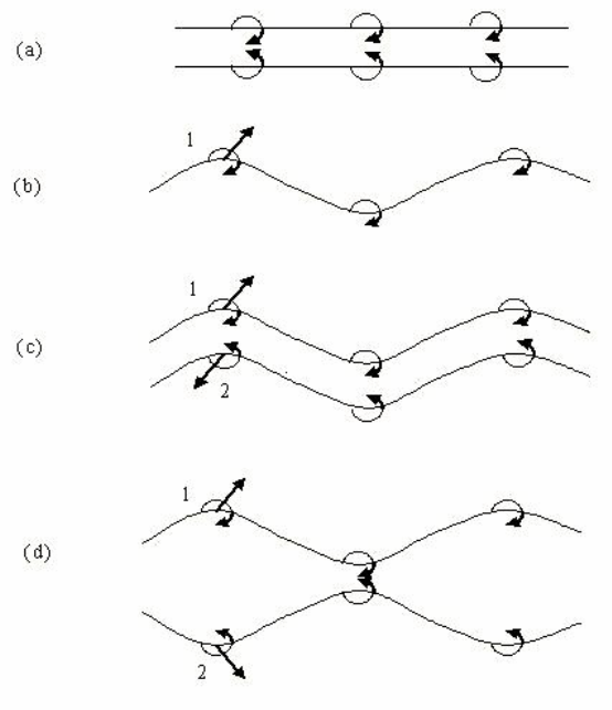
Figure 8: Induced velocity field of the symmetric and asymmetric modes. (a): Idealization of the base flow of the wake into two shear layers of opposite sign. (b): Perturbed upper shear layer. (c): Induced velocities in the asymmetric mode. Note that they cancel to lowest order. (d): Induced velocities in the symmetric mode. Superposition enhances the amplitude at both points 1 and 2.

This linear absolute instability takes place in the intermediate and far field and acts as a source of excitation for the pair of steady recirculating eddies in the lee of the cylinder. The onset of a time periodic flow, a supercritical Hopf bifurcation ([31], [32]) indicates that in the end the vortices are shed alternatively from the separated streamlines above and below the cylinder forming the Von Karman vortex street. The vortex street is the stable configuration after the bifurcation has taken place. It has the symmetry of a traveling sinuous mode, which indicates asymmetry up-and-down of the cylinder. Thus, it can be observed that, also in the context of the vortex shedding, asymmetry shows higher stability properties with respect to symmetry.

3.3 Asymptotic fate and comparison with modal analysis

Figure 9 presents a comparison between the initial-value problem and the asymptotic theory results represented by the zero order Orr-Sommerfeld problem ([24]) in terms of temporal growth rate $r$ and pulsation $\omega$.

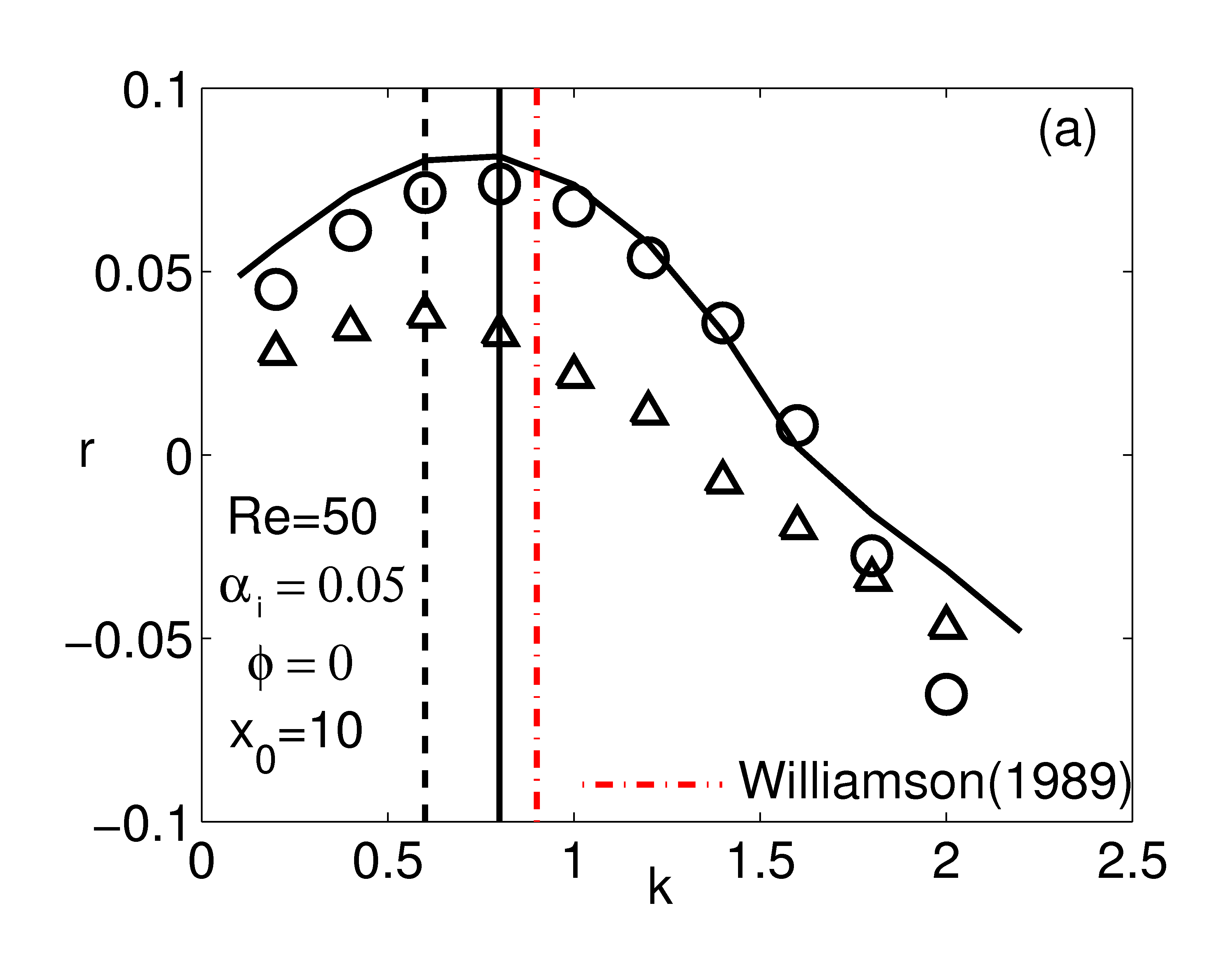
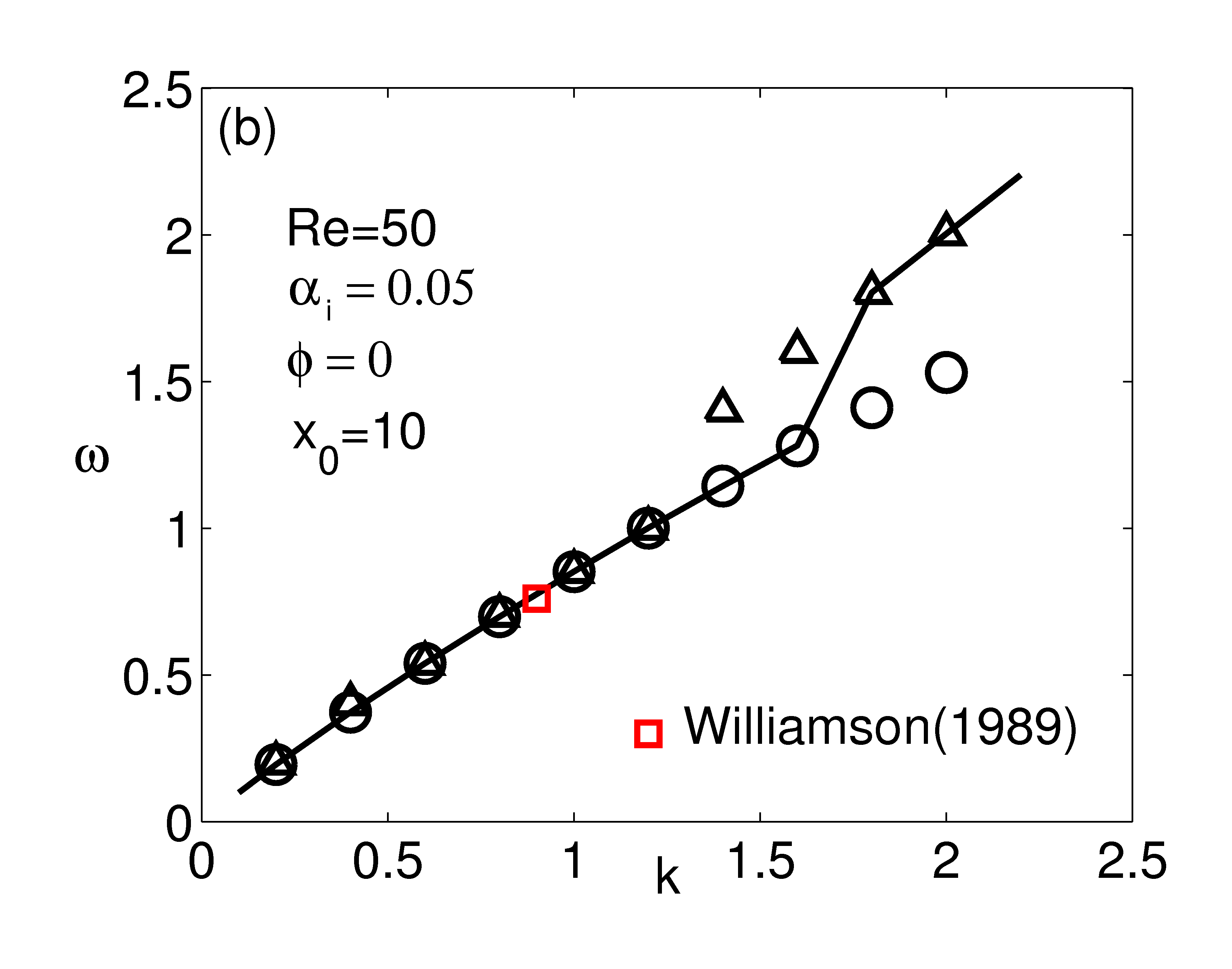
Figure 9: (a) Temporal growth rate and (b) pulsation. Comparison among the asymptotic results obtained by the IVP analysis (circles: symmetric perturbation; triangles: asymmetric perturbation) and the normal mode analysis (solid lines, see [24]. The asymptotic values for the IVP analysis are determined when the condition $dr/dt<\epsilon$ ($\epsilon\sim 10^{-4}$) is satisfied. For the symmetric perturbations the asymptote was reached before 50 time scales were elapsed, for the asymmetric perturbation the asymptote was determined after 500 time scales were elapsed.

In fig. 9 the imaginary part $\alpha_{i}$ of the complex longitudinal wavenumber is fixed, and differing polar wavenumbers ($k=\alpha_{r}$) are considered. For both the symmetric and asymmetric arbitrary disturbances here considered, a good agreement with the stability characteristics given by the multiscale near-parallel Orr-Sommerfeld theory can be observed. However, it should be noted that the wave number corresponding to the maximum growth factor in the case of asymmetric perturbations is about 15% lower than that obtained in the case of symmetric perturbations and that obtained by the normal mode analysis. When the perturbations are asymmetric, the transient is very long, of the order of hundreds time scales. This difference can be due either to the fact that the true asymptote was not yet reached, or to the fact that the extent of the numerical errors in the integration of the equations is higher than that obtained in the case of symmetric transients, which last only a few dozen time scales. Note that this satisfactory agreement is observed by using arbitrary initial conditions in terms of elements of the trigonometrical Schauder basis for the $L^{2}$ space, and not by considering as initial condition the most unstable waves given by the Orr-Sommerfeld dispersion relation. Moreover, a maximum of the perturbation energy (in terms of $r$) is found around $k=0.8$ and confirmed by both the analyses.

As shown in fig. 9, we have also contrasted our results with the laboratory experimental results obtained in 1989 by Williamson[27], who gave a quantitative determination of the Strouhal number and wavelength of the vortex shedding – oblique and parallel modes – of a circular cylinder at low Reynolds number. The comparison is quantitatively good, because it shows that a wave number close to the wave number that theoretically has the maximum growth rate at $Re=50$ (see part a of fig. 9) has a – theoretically deduced – frequency which is very close to the frequency measured in the laboratory. At this point, also the laboratory experimental uncertainty, globally of the order of a $\pm 10\%$ in an accurate measurement set up, should be introduced. The uncertainty associated to the laboratory method and to the theoretical model (estimated through the difference between the position of the maximum growth rate showed by the two cases of asymmetric and symmetric perturbation) overlaps, which confirms the quality of this comparison. The same quantitative agreement is observed also at $Re=100$.

4 Conclusions

The three-dimensional stability analysis of the intermediate asymptotics of the 2D bluff-body viscous growing wake was considered as an initial-value problem. The velocity-vorticity formulation was used. The perturbative equations are Laplace-Fourier transformed in the plane normal to the growing basic flow. The Laplace transform allows for the use of a damped perturbation in the streamwise direction as initial condition. In this regard, the introduction of the imaginary part of the longitudinal wavenumber (the spatial damping rate) was done to explicitly include in the perturbation, which otherwise would have been longitudinally homogeneous, a degree of freedom associated to the spatial evolution of the system.

An important point is that the vorticity-velocity formulation, Fourier-Laplace transformation, allows (over a reasonable lapse of computing time) for the following of the temporal evolution over hundred of basic flow time scales and thus to observe very long transients. Such a limiting behaviour would not have been so easily reached by means of the direct numerical integration of the linearized governing equations of the motion.

Two main transient scenarios have been observed in the region of the wake where the entrainment is present, the region in between $x_{0}=10$ diameters (intermediate) and $x_{0}=50$ diameters (far field), for a $Re$ number equal to $50$ and $100$. A long transient, where an initial growth smoothly levels off and is followed either by an ultimate damping or by a slow amplification for both oblique or 2D waves, and a short transient where the growth or the damping is monotone. The most important parameters affecting these configurations are the angle of obliquity, the symmetry, the polar wavenumber and the spatial damping rate. While the symmetry of the disturbance is remarkably influencing the transient behaviour leaving inalterate the asymptotic fate, a variation of the obliquity, of the polar wavenumber and of the spatial damping rate can significantly change the early trend as well as the final stability configuration. Interesting phenomena are observed. A first one is that, in the case of asymmetric longitudinal or oblique perturbations, the system exhibits two periodic patterns, a first, of transient nature, and a second one of asymptotic nature. A second phenomenon is that, in the case of an orthogonal perturbation, albeit always initially set equal to zero, the transversal vorticity component is the vorticity component which grows faster. The third phenomenology is linked to the magnitude of the spatial damping rate. Perturbations that are more rapidly damped in space lead to a larger growth in time.

For disturbances aligned with the flow, the asymptotic behaviour is shown to be in excellent agreement with the zero order results of spatio-temporal multiscale modal analyses and with the laboratory determined frequency and wave length of the parallel vortex shedding at $Re=50$ and $100$. It should be noted that the agreement between the initial value problem results and the normal mode theory is obtained not using as initial condition the most unstable wave given by the Orr-Sommerfeld dispersion relation at any section of the wake, but arbitrary initial conditions in terms of elements of the trigonometrical Schauder basis for the $L^{2}$ space.

References

- [1] K. M. Butler and B. F. Farrell. Three-dimensional optimal perturbations in viscous shear flow, Phys. Fluids A. 4: 1637–1650 (1992).
- [2] W. O. Criminale and P. G. Drazin. The evolution of linearized perturbations of parallel shear flows, Stud. in Applied Math. 83: 123–157 (1990).
- [3] W. O. Criminale, B. Long and M. Zhu. General three-dimensional disturbances to inviscid Couette flow, Stud. in Applied Math. 85: 249–267 (1991).
- [4] A. Sommerfeld. Partial Differential Equations in Physics, Lectures in Theoretical Physics. 6, Academic Press (1949).
- [5] D. J. Benney and L. H. Gustavsson. A new mechanism for linear and non-linear hydrodynamic instability, Stud. in Applied Math. 64: 185–209 (1981).
- [6] W. O. Criminale, T. L. Jackson, D. G. Lasseigne and R. D. Joslin. Perturbation dynamics in viscous channel flows, J. Fluid Mech. 339: 55–75 (1997).
- [7] L. H.Gustavsson. Energy growth of three-dimensional disturbances in plane Poiseuille flow, J. Fluid Mech. 224: 241–260 (1991).
- [8] L. Bergstrom. Evolution of laminar disturbances in pipe Poiseuille flow, Eur. J. Mech. B/Fluids. 12: 749–768 (1993).
- [9] P. J. Schmid and D. S. Henningson. Optimal energy density growth in Hagen-Poiseuille flow, J. Fluid Mech. 277: 197–225 (1994).
- [10] P. J. Schmid. Nonmodal Stability Theory, Ann. Rev. Fluid Mech. 39: 129–162 (2007).
- [11] D. G. Lasseigne, R. D. Joslin, T. L. Jackson and W. O. Criminale. The transient period for boundary layer disturbances, J. Fluid Mech. 381: 89–119 (1999).
- [12] L. S. Hultgren and L. H. Gustavsson. Algebraic growth of disturbance in a laminar boundary layer, Phys. Fluids. 24: 1000–1004 (1981).
- [13] P. Corbett and A. Bottaro. Optimal perturbations for boundary layers subject to stream-wise pressure gradient, Phys. Fluids. 12 (1): 366–374 (2000).
- [14] W. O. Criminale and P. G. Drazin. The initial-value problem for a modeled boundary layer, Phys. Fluids. 12: 366–374 (2000).
- [15] Y. Bun and W. O. Criminale. Early-period dynamics of an incompressible mixing layer, J. Fluid Mech. 273: 31–82 (1994).
- [16] W. O. Criminale, T. L. Jackson and D. G. Lasseigne. Towards enhancing and delaying disturbances in free shear flows, J. Fluid Mech. 294: 283–300 (1995).
- [17] G. E. Mattingly and W. O. Criminale. The stability of an incompressible two-dimensional wake, J. Fluid Mech. 51: 233–272 (1972).
- [18] G. S. Triantafyllou, M. S. Triantafyllou and C. Chryssostomidis. On the formation of vortex street behind stationary cylinders, J. Fluid Mech. 170: 461–477 (1986).
- [19] L. S. Hultgren and A. K. Aggarwal. Absolute instability of the Gaussian wake profile, Phys. Fluids. 30: 3383–3387 (1987).
- [20] P. Huerre and P. A. Monkewitz. Local and global instabilities in spatially developing flows, Ann. Rev. Fluid Mech. 22: 473–537. (1990).
- [21] M. Belan and D. Tordella. Asymptotic expansions for two-dimensional symmetrical laminar wakes, ZAMM. 82: 219–234 (2002).
- [22] D. Tordella and M. Belan. A new matched asymptotic expansion for the intermediate and far flow behind a finite body, Phys. Fluids. 15: 1897–1906 (2003).
- [23] M.Belan and D. Tordella. Convective instability in wake intermediate asymptotics, J. Fluid Mech. 552: 127–136 (2006).
- [24] D. Tordella, S. Scarsoglio and M. Belan. A synthetic perturbative hypothesis for multiscale analysis of convective wake instability, Phys. Fluids. 18: 054105 (2006).
- [25] P. J. Schmid and D. S. Henningson. Stability and transition in shear flows. New York: Springer - Verlag (2001).
- [26] W. O. Criminale, T. L. Jackson and R. D. Joslin, Theory and computation in Hydrodynamic Stability. Cambridge: Cambridge Univeristy Press (2003).
- [27] C. H. K. Williamson. Oblique and parallel modes of vortex shedding in the wake of a circular cylinder at low Reynolds numbers, J. Fluid Mech. 206: 579–627 (1989).
- [28] G. I. Barenblatt. Scaling, Self-similarity, and Intermediate Asymptotics, Cambridge University Press. Cambridge UK (1966).
- [29] G. B. Whitham. Linear and nonlinear waves, New York, Wiley. (1974).
- [30] G. Coppola and L. De Luca. On transient growth oscillations in linear models, Phys. Fluids. 18, 078104 (2006).
- [31] T. L. Jackson. Effect of thermal-expansion on the stability of 2-reactant flames, Combustion Science and Technology. 53: 51–54 (1987).
- [32] M. Provansal, C. Mathis and L. Boyer. Benard-Von Karman instability - Transient and forced regimes, J. Fluid Mech. 182: 1–22 (1987).