Isotropic transformation optics:
approximate acoustic and quantum cloaking

Abstract

Transformation optics constructions have allowed the design of electromagnetic, acoustic and quantum parameters that steer waves around a region without penetrating it, so that the region is hidden from external observations. The material parameters are anisotropic, and singular at the interface between the cloaked and uncloaked regions, making physical realization a challenge. We address this problem by showing how to construct isotropic and nonsingular parameters that give approximate cloaking to any desired degree of accuracy for electrostatic, acoustic and quantum waves. The techniques used here may be applicable to a wider range of transformation optics designs.

For the Helmholtz equation, cloaking is possible outside a discrete set of frequencies or energies, namely the Neumann eigenvalues of the cloaked region. For the frequencies or energies corresponding to the Neumann eigenvalues of the cloaked region, the ideal cloak supports trapped states; near these energies, an approximate cloak supports almost trapped states. This is in fact a useful feature, and we conclude by giving several quantum mechanical applications.

1 Introduction

Cloaking devices designs based on transformation optics require anisotropic and singular material parameters, whether the conductivity (electrostatic) [27, 28], index of refraction (Helmholtz) [40, 19], permittivity and permeability (Maxwell) [47, 19], mass tensor (acoustic) [9, 15, 23, 46], or effective mass (Schrödinger)[54]. The same is true for other transformation optics designs, such as those motivated by general relativity [41]; field rotators [8]; concentrators [43]; electromagnetic wormholes [20, 22]; or beam splitters [48]. Both the anisotropy and singularity present serious challenges in trying to physically realize such theoretical plans using metamaterials. In this paper, we give a general method, isotropic transformation optics, for dealing with both of these problems; we describe it in some detail in the context of cloaking, but it should also be applicable to a wider range of transformation optics-based designs.

A well known phenomenon in effective medium theory is that homogenization of isotropic material parameters may lead, in the small-scale limit, to anisotropic ones [44]. Using ideas from [45, 1, 11] and elsewhere, we show how to exploit this to find cloaking material parameters that are at once both isotropic and nonsingular, at the price of replacing perfect cloaking with approximate cloaking (of arbitrary accuracy). This method, starting with transformation optics-based designs and constructing approximations to them, first by nonsingular, but still anisotropic, material parameters, and then by nonsingular isotropic parameters, seems to be a very flexible tool for creating physically realistic theoretical designs, easier to implement than the ideal ones due to the relatively tame nature of the materials needed, yet essentially capturing the desired effect on waves.

In ideal cloaking, for any wave propagation governed by the Helmholtz equation at frequency $\omega$, there is a dichotomy [19, Thm. 1] between generic values of $\omega$, for which the waves must vanish within the cloaked region $D$, and the discrete set of Neumann eigenvalues of $D$, for which there exist trapped states: waves which are zero outside of $D$ and equal to a Neumann eigenfunction within $D$. In the approximate cloaking resulting from isotropic transformation optics that we will describe, trapped states for the limiting ideal cloak give rise to almost trapped states for the approximate cloaks. The existence of these should be considered as a feature, not a bug; we discuss this further in Sec. 4.2 and give applications in [25].

We start by considering isotropic transformation optics for acoustic (and hence, at frequency zero, electrostatic) cloaking. First recall ideal cloaking for the Helmholtz equation. For a Riemannian metric $g=(g_{ij})$ in $n$-dimensional space, the Helmholtz equation with source term is

$$\frac{1}{\sqrt{|g|}}\sum_{i,j=1}^{n}\frac{\partial}{\partial x_{i}}\left(\sqrt{|g|}\,g^{ij}\frac{\partial u}{\partial x_{j}}\right)+\omega^{2}u=p,$$ (1)

where $|g|=\hbox{det}(g_{ij})$ and $(g^{ij})=g^{-1}=(g_{ij})^{-1}$. In the acoustic equation, for which ideal 3D spherical cloaking was described by Chen and Chan [9] and Cummer, et al., [15], $\sqrt{|g|}g^{ij}$ represents the anisotropic density and $\sqrt{|g|}$ the bulk modulus.

In [19], we showed that the singular cloaking metrics $g$ for electrostatics constructed in [27, 28], giving the same boundary measurements of electrostatic potentials as the Euclidian metric $g_{0}=(\delta_{ij})$, also cloak with respect to solutions of the Helmholtz equation at any nonzero frequency $\omega$ and with any source $p$. An example in 3D, with respect to spherical coordinates $(r,\theta,\phi)$, is

$$(g^{jk})=\left(\begin{array}[]{ccc}2(r-1)^{2}\sin\theta&0&0\\ 0&2\sin\theta&0\\ 0&0&2(\sin\theta)^{-1}\\ \end{array}\right)$$ (5)

on $B_{2}-B_{1}=\{1<r\leq 2\}$, with the cloaked region being the ball $B_{1}=\{0\leq r\leq 1\}$. This $g$ is the image of $g_{0}$ under the singular transformation $(r,\theta,\phi)=F(r^{\prime},\theta^{\prime},\phi^{\prime})$ defined by $r=1+\frac{r^{\prime}}{2},\,\theta=\theta^{\prime},\,\phi=\phi^{\prime},\,0<r^{\prime}\leq 2$, which blows up the point $r^{\prime}=0$ to the cloaking surface $\Sigma=\{r=1\}$. The same transformation was used by Pendry, Schurig and Smith [47] for Maxwell’s equations and gives rise to the cloaking structure that is referred to in [19] as the single coating. It was shown in [19, Thm.1] that if the cloaked region is given any nondegenerate metric, then finite energy waves $u$ that satisfy the Helmholtz equation (1) on $B_{2}$ in the sense of distributions (cf. Sec. 2.2 below) have the same set of Cauchy data at $r=2$, i.e., the same acoustic boundary measurements, as do the solutions for the Helmholtz equation for $g_{0}$ with source term $p\circ F$. The part of $p$ supported within the cloaked region is undetectable at $r=2$, while the part of $p$ outside $\Sigma$ appears to be shifted by the transformation $F$; cf. [56]. Furthermore, on the inner side $\Sigma^{-}$ of the cloaking surface, the normal derivative of $u$ must vanish, so that within $B_{1}$ the acoustic waves propagate as if $\Sigma$ were lined with a sound–hard surface. Within $B_{1}$, $u$ can be any Neumann eigenfunction; if $-\omega^{2}$ is not an eigenvalue, then the wave must vanish on $B_{1}$, while if it is, then $u$ can equal any associated eigenfunction there, leading to what we refer to as a trapped state of the cloak.

In Sec. 2 we introduce isotropic transformation optics in the setting of acoustics, starting by approximating the ideal singular anisotropic density and bulk modulus by nonsingular anisotropic parameters. Then, using a homogeneization argument [45, 1], we approximate these nonsingular anisotropic parameters by nonsingular isotropic ones. This yields almost, or approximate, invisibility in the sense that the boundary observations for the resulting acoustic parameters converge to the corresponding ones for a homogeneous, isotropic medium.

In Sec. 3 we consider the quantum mechanical scattering problem for the time-independent Schrödinger equation at energy $E$,

$$(-\nabla^{2}+V(x))\psi(x)=E\psi(x),\quad x\in\mathbb{R}^{d},$$ (6)

$$\psi(x)=\exp(iE^{1/2}x\cdotp\theta)+\psi_{sc}(x),$$

where $\theta\in\mathbb{R}^{d}$, $|\theta|=1$, and $\psi_{sc}(x)$ satisfies the Sommerfeld radiation condition. By a gauge transformation, we can reduce an isotropic acoustic equation to a Schrödinger equation. In this paper we restrict ourselves to the case when the potential $V$ is compactly supported, so that

$$\psi_{sc}(x)=\frac{a_{V}(E,{x}/{|x|},\theta)}{|x|^{\frac{d-1}{2}}}\cdot e^{i\lambda|x|}+{\cal O}\Big{(}\frac{1}{|x|^{\frac{d}{2}}}\Big{)},\quad\hbox{as }|x|\to\infty.$$

The function $a_{V}(E,\theta^{\prime},\theta)$ is the scattering amplitude at energy $E$ of the potential $V$. The inverse scattering problem consists of determination of $V$ from the scattering amplitude. As $V$ is compactly supported, this inverse problem is equivalent to the problem of determination of $V$ from boundary measurements. Indeed, if $V$ is supported in a domain $\Omega$, we define the Dirichlet-to-Neumann (DN) operator $\Lambda_{V}(E)$ at energy $E$ for the potential $V$ as follows. For any smooth function $f$ on $\partial\Omega$, we set

$$\Lambda_{V}(E)f=\partial_{\nu}\psi|_{\partial\Omega}$$

where $\psi$ is the solution of the Dirichlet boundary value problem

$$(-\nabla^{2}+V)\psi=E\psi,\,\,\psi|_{\partial\Omega}=f.$$

(Of course, $\Lambda_{V}(E)=\Lambda_{V-E}(0)$.) Knowing $\Lambda_{V}(E)$ is equivalent to knowing $a_{V}(E,\theta^{\prime},\theta)$ for all $(\theta^{\prime},\theta)\in{\mathbb{S}}^{d-1}\times{\mathbb{S}}^{d-1}$. Roughly speaking, $\Lambda_{V}(E)$ can be considered as knowledge of all external observations of $V$ at energy $E$ [5].

In Sec. 4 we also consider the magnetic Schrödinger equation with magnetic potential $A$ and electric potential $V$,

$$(-(\nabla+iA)^{2}+V-E)\psi=0,\quad\psi|_{\partial\Omega}=f,$$

which defines the DN operator,

$$\Lambda_{V,A}(E)(f)=\partial_{\nu}\psi|_{\partial\Omega}+i(A\cdot\nu)f.$$

There is an enormous literature on unique determination of a potential, whether from scattering data or from boundary measurements of solutions of the associated Schrödinger equation. In [51] it was shown that an $L^{\infty}$ potential is determined by the associated DN operator, and [39] and [7] extended this to rougher potentials. In dimension $d=2$, it has been shown recently that uniqueness holds if $V$ is merely in $L^{p},p>2$ [6].

On the other hand, for $d=2$ and each $E>0$, there are continuous families of rapidly decreasing (but noncompactly supported) potentials which are transparent, i.e., for which the scattering amplitude $a_{V}(E,\theta^{\prime},\theta)$ vanishes at a fixed energy $E$, $a_{V}(E,\theta^{\prime},\theta)\equiv a_{0}(E,\theta^{\prime},\theta)=0$ [29]. More recently, [32] described central potentials transparent on the level of the ray geometry.

Recently, Zhang, et al., [54] have described an ideal quantum mechanical cloak at any fixed energy $E$ and proposed a physical implementation. The construction starts with a homogeneous, isotropic mass tensor $\widehat{m}_{0}$ and potential $V_{0}\equiv 0$, and subjects this pair to the same singular transformation (“blowing up a point”) as was used in [27, 28, 47]. The resulting cloaking mass-density tensor $\widehat{m}$ and potential $V$ yield a Schrödinger equation that is the Helmholtz equation (at frequency $\omega=\sqrt{E})$ for the corresponding singular Riemannian metric, thus covered by the analysis of cloaking for the Helmholtz equation in [19, Sec. 3]. The cloaking mass-density tensor $\widehat{m}$ and potential are both singular, and $\widehat{m}$ infinitely anisotropic, at $\Sigma$, combining to make such a cloak difficult to implement, with the proposal in [54] involving ultracold atoms trapped in an optical lattice.

In this paper, we consider the problem in dimension $d=3$. For each energy $E$, we construct a family $\{V_{n}^{E}\}_{n=1}^{\infty}$ of bounded potentials, supported in the annular region $B_{3}-B_{1}$, which act as an approximate invisibility cloak: for any potential $W$ on $B_{1}$, the scattering amplitudes $a_{V_{n}^{E}+W}(E,\theta^{\prime},\theta)\to 0$ as $n\to\infty$. Thus, when surrounded by the cloaking potentials $V_{n}^{E}$, the potential $W$ is undetectable by waves at energy $E$, asymptotically in $n$. Furthermore, $E$ either is or is not a Neumann eigenvalue for $W$ on the cloaked region. In the latter case, with high probability the approximate cloak keeps particles of energy $E$ from entering the cloaked region; i.e., the cloak is effective at energy $E$. In the former case, the cloaked region supports “almost trapped” states, accepting and binding such particles and thereby functioning as a new type of ion trap. Furthermore, the trap is magnetically tunable: application of a homogeneous magnetic field allows one to switch between the two behaviors [25].

In Sec. 4 we consider several applications to quantum mechanics of this approach. In the first, we study the magnetic Schrödinger equation and construct a family of potentials which, when combined with a fixed homogeneous magnetic field, make the matter waves behave as if the potentials were almost zero and the magnetic potential were blowing up near a point, thus giving the illusion of a locally singular magnetic field. In the second, we describe “almost trapped” states which are largely concentrated in the cloaked region. For the third application, we use the same basic idea of isotropic transformation optics but we replace the single coating construction used earlier by the double coating construction of [19], corresponding to metamaterials deployed on both sides of the cloaking surface, to make matter waves behave as if confined to a three dimensional sphere, ${\mathbb{S}}^{3}$.

Full mathematical proofs will appear elsewhere [24]. The authors are grateful to A. Cherkaev and V. Smyshlyaev for useful discussions on homogenization, to S. Siltanen for help with the numerics, and to the anonymous referees for constructive criticism and additional references.

2 Cloaking for the acoustic equation

2.1 Background

Our analysis is closely related to the inverse problem for electrostatics, or Calderón’s conductivity problem. Let $\Omega\subset\mathbb{R}^{d}$ be a domain, at the boundary of which electrostatic measurements are to be made, and denote by $\sigma(x)$ the anisotropic conductivity within. In the absence of sources, an electrostatic potential $u$ satisfies a divergence form equation,

$$\nabla\cdot\sigma\nabla u=0$$ (7)

on $\Omega$. To uniquely fix the solution $u$ it is enough to give its value, $f$, on the boundary. In the idealized case, one measures, for all voltage distributions $u|_{\partial\Omega}=f$ on the boundary the corresponding current fluxes, $\nu\cdotp\sigma\nabla u$, where $\nu$ is the exterior unit normal to $\partial\Omega$. Mathematically this amounts to the knowledge of the Dirichlet–Neumann (DN) map, $\Lambda_{\sigma}$. corresponding to $\sigma$, i.e., the map taking the Dirichlet boundary values of the solution to (7) to the corresponding Neumann boundary values,

$$\Lambda_{\sigma}:\ \ u|_{\partial\Omega}\mapsto\nu\cdotp\sigma\nabla u|_{\partial\Omega}.$$ (8)

If $F:\Omega\to\Omega,\quad F=(F^{1},\dots,F^{d})$, is a diffeomorphism with $F|_{\partial\Omega}=\hbox{Identity}$, then by making the change of variables $y=F(x)$ and setting $u=v\circ F^{-1}$, we obtain

$$\nabla\cdot\widetilde{\sigma}\nabla v=0,$$ (9)

where $\widetilde{\sigma}=F_{*}\sigma$ is the push forward of $\sigma$ in $F$,

$$(F_{*}\sigma)^{jk}(y)=\left.\frac{1}{\hbox{det}[\frac{\partial F^{j}}{\partial x^{k}}(x)]}\sum_{p,q=1}^{d}\frac{\partial F^{j}}{\partial x^{p}}(x)\,\frac{\partial F^{k}}{\partial x^{q}}(x)\sigma^{pq}(x)\right|_{x=F^{-1}(y)}.$$ (10)

This can be used to show that

$$\Lambda_{F_{*}\sigma}=\Lambda_{\sigma}.$$

Thus, there is a large (infinite-dimensional) family of conductivities which all give rise to the same electrostatic measurements at the boundary. This observation is due to Luc Tartar (see [37] for an account.) Calderón’s inverse problem for anisotropic conductivities is then the question of whether two conductivities with the same DN operator must be push-forwards of each other. There are a number of positive results in this direction, but it was shown in [27, 28] that, if one allows singular maps, then in fact there counterexamples, i.e., conductivities that are undetectable to electrostatic measurements at the boundary. See [36] for $d=2$.

¿From now on, for simplicity we will restrict ourselves to the three dimensional case. For each $R>0$, let $B_{R}=\{|x|\leq R\}$ and $\Sigma_{R}=\{|x|=R\}$ be the central ball and sphere of radius $R$, resp., in $\mathbb{R}^{3}$, and let ${\it O}=(0,0,0)$ denote the origin. To construct an invisibility cloak, for simplicity we use the specific singular coordinate transformation $F:\mathbb{R}^{3}-\{{\it O}\}\to\mathbb{R}^{3}-B_{1},$ given by

$$x=F(y):=\left\{\begin{array}[]{cl}y,&\hbox{for }|y|>2,\\ \left(1+\frac{|y|}{2}\right)\frac{y}{|y|},&\hbox{for }0<|y|\leq 2.\end{array}\right.$$ (13)

Letting $\sigma_{0}=1$ be the homogeneous isotropic conductivity on $\mathbb{R}^{3}$, $F$ then defines a conductivity $\sigma$ on $\mathbb{R}^{3}-B_{1}$ by the formula

$$\sigma^{jk}(x):=(F_{*}\sigma_{0})^{jk}(x),$$ (14)

cf. (10). More explicitly, the matrix $\sigma=[\sigma^{jk}]_{j,k=1}^{3}$ is

$$\sigma(x) = 2|x|^{-2}(|x|-1)^{2}\Pi(x)+2(I-\Pi(x)),\quad 1<|x|<2,$$

where $\Pi(x):\mathbb{R}^{3}\to\mathbb{R}^{3}$ is the projection to the radial direction, defined by

$$\Pi(x)\,v=\left(v\,\cdotp\frac{x}{|x|}\right)\frac{x}{|x|},$$ (15)

i.e., $\Pi(x)$ is represented by the matrix $|x|^{-2}xx^{t}$, cf. [36].

One sees that $\sigma(x)$ is singular, as one of its eigenvalues, namely the one corresponding to the radial direction, tends to $0$ as $|x|\searrow 1$. We can then extend $\sigma$ to $B_{1}$ as an arbitrary smooth, nondegenerate (bounded from above and below) conductivity there. Let $\Omega=B_{3}$; the conductivity $\sigma$ is then a cloaking conductivity on $\Omega$, as it is indistinguishable from $\sigma_{0}$, vis-a-vis electrostatic boundary measurements of electrostatic potentials, treated rigorously as bounded, distributional solutions of the degenerate elliptic boundary value problem corresponding to $\sigma$ [27, 28].

The same construction of $\sigma|_{\Omega-B_{1}}$ was proposed in Pendry, Schurig and Smith [47] to cloak the region $B_{1}$ from observation by electromagnetic waves at a positive frequency; see also Leonhardt [40] for a related approach for Helmholtz in $\mathbb{R}^{2}$.

2.2 Cloaking for Helmholtz: ideal acoustic cloaks

The cloaking conductivity $\sigma$ above corresponds to a Riemannian metric $g_{jk}$ that is related to $\sigma^{ij}$ by

$$\sigma^{ij}(x)=|g(x)|^{1/2}g^{ij}(x),\quad|g|=\left(\hbox{det}[\sigma^{ij}]\right)^{2}$$ (16)

where $[g^{jk}(x)]$ is the inverse matrix of $[g_{jk}(x)]$ and $|g(x)|=\hbox{det}[g_{jk}(x)]$. The Helmholtz equation, with source term $p$, corresponding to this cloaking metric has the form

$$\sum_{j,k=1}^{3}|g(x)|^{-1/2}\frac{\partial}{\partial x^{j}}(|g(x)|^{1/2}g^{jk}(x)\frac{\partial}{\partial x^{k}}u)+\omega^{2}u=p\quad\hbox{on }\Omega,$$ (17)

$$u|_{\partial\Omega}=f.$$

For now, $g$ is allowed to be an arbitrary nonsingular Riemannian metric, $g_{inn}$, on $B_{1}$. Reinterpreting the conductivity tensor $\sigma$ as a mass tensor ( which has the same transformation law (10) ) and $|g|^{\frac{1}{2}}$ as the bulk modulus parameter, (17) becomes an acoustic equation,

$$\left(\nabla\cdotp\sigma\nabla+\omega^{2}|g|^{\frac{1}{2}}\right)u=p(x)|g|^{\frac{1}{2}}\quad\hbox{on }\Omega,$$ (18)

$$u|_{\partial\Omega}=f.$$

This is the form of the acoustic wave equation considered in [9, 15]; see also [14] for $d=2$, and [46] for a somewhat different approach. As $\sigma$ is singular at the cloaking surface $\Sigma:=\Sigma_{1}=\partial B_{1}$, one has to carefully define what one means by “waves”, that is by solutions to (17) or (18). Let us recall the precise definition of the solution to (17) or (18), discussed in detail in [19]. We say that $u$ is a finite energy solution of the Helmholtz equation (17) or the acoustic equation (18) if

1. $u$ is square integrable with respect to the metric, i.e., is in the weighted $L^{2}$-space,

   $$u\in L^{2}_{g}(\Omega)=\{u:\ \|u\|^{2}_{g}:=\int_{\Omega}\,dx\,|g|^{1/2}|u|^{2}<\infty\};$$

2. the energy of $u$ is finite,

   $$\|\nabla u\|_{g}^{2}:=\int_{\Omega}\,dx\,|g|^{1/2}g^{ij}\partial_{i}u\partial_{j}u<\infty;$$

3. $u$ satisfies the Dirichlet boundary condition $u|_{\partial\Omega}=f$; and

4. the equation (18) is valid in the weak distributional sense, i.e., for all ${\psi}\in C^{\infty}_{0}(\Omega)$

   $$\int_{\Omega}\,dx\,[-(|g|^{1/2}g^{ij}\partial_{i}u)\partial_{j}{\psi}+\omega^{2}u{\psi}|g|^{1/2}]=\int_{\Omega}\,dx\,p(x){\psi}(x)|g|^{1/2}.$$ (19)

This last can be interpreted as saying that any smooth superposition of point measurements of $u$ satisfies the same integral identity as it would for a classical solution. We also note that, since $g$ is singular, the term $|g|^{1/2}g^{ij}\partial_{i}u$ must also be defined in an appropriate weak sense.

It was shown in [19, Thm. 1] that if $u$ is the finite energy solution of the acoustic equation (18), then $u(x)$ defines two functions $v^{+}(y),\,y\in\Omega$, and $v^{-}(y),\,y\in B_{1}$, by the formulae

$$u(x)=\left\{\begin{array}[]{cl}v^{+}(y),&\hbox{where $x=F(y)$, for }1<|x|<3,\\ v^{-}(y),&\hbox{where $x=y$, for }0<|x|<1.\end{array}\right.$$ (22)

These functions satisfy the following boundary value problems:

$$(\nabla^{2}+\omega^{2})v^{+}(y) = \widetilde{p}(y):=p(F(y))\quad\hbox{in }\Omega,$$ (23)

$$v^{+}|_{\partial\Omega} = f,$$

and

$$(\nabla^{2}_{g_{inn}}+\omega^{2}|g_{inn}|^{1/2})v^{-}(y) = |g_{inn}|^{1/2}p(y)\quad\hbox{in }B_{1},$$ (24)

$$\partial_{\nu}v^{-}|_{\partial B_{1}} = 0$$

where $\partial_{\nu}u=\partial_{r}u$ denotes the normal derivative on $\partial B_{1}$.

In the absence of sources within the cloaked region, (24) leads, as mentioned in the introduction, to the phenomenon of trapped states: If $-\omega^{2}$ is not a Neumann eigenvalue for $(B_{1},g_{inn})$, then $v^{-}\equiv 0$ on $B_{1}$, the waves do not enter $B_{1}$, and cloaking as generally understood holds. On the other hand, if $-\omega^{2}$ is an eigenvalue, then $v^{-}$ can be any function in the associated eigenspace; indeed, one can have $v^{+}\equiv 0$, in which case the total wave $u$ behaves as a bound state for the cloak, concentrated in $B_{1}$; for simplicity, we refer to this as a trapped state of the ideal cloak.

2.3 Nonsingular approximate acoustic cloak

Next, consider nonsingular approximations to the ideal cloak, which are more physically realizable by virtue of having bounded anisotropy ratio; see [49, 21, 36] for analyses of cloaking from the point of view of similar truncations. Studying the behavior of solutions to the corresponding boundary value problems near the cloaking surface, as these nonsingular approximately cloaking conductivities tend to the ideal $\sigma$, we will see that the Neumann boundary condition appears in (24) on the cloaked region $B_{1}$. At the present time, for mathematical proofs [24] of some of the results below we assume that $\sigma$ be chosen to be the homogeneous, isotropic conductivity, $\sigma=\kappa\sigma_{0}$ inside $B_{1}$, i.e., $\sigma^{jk}(x)=\kappa\delta^{jk}$, with $\kappa\geq 2$ a constant such that $-\omega^{2}$ is not a Neumann eigenvalue on $B_{1}$. The first assumption is not needed for physical arguments, but the second is.

To start, let $1<R<2$, $\rho:=2(R-1)$ and introduce the coordinate transformation $F_{R}:\mathbb{R}^{3}-B_{\rho}\to\mathbb{R}^{3}-B_{R}$,

$$x:=F_{R}(y)=\left\{\begin{array}[]{cl}y,&\hbox{for }|y|>2,\\ \left(1+\frac{|y|}{2}\right)\frac{y}{|y|},&\hbox{for }\rho<|y|\leq 2.\end{array}\right.$$

We define the corresponding approximate conductivity, $\sigma_{R}$ as

$$\sigma^{jk}_{R}(x)=\left\{\begin{array}[]{cl }\sigma^{jk}(x)&\hbox{for }|x|>R,\\ \kappa\delta^{jk},&\hbox{for }|x|\leq R.\end{array}\right.$$ (28)

Note that then $\sigma^{jk}(x)=\left(\left(F_{R}\right)_{*}\sigma_{0}\right)^{jk}(x)$ for $|x|>R$, where $\sigma_{0}\equiv 1$ is the homogeneous, isotropic conductivity (or mass density) tensor, Observe that, for each $R>1$, the conductivity $\sigma_{R}$ is nonsingular, i.e., is bounded from above and below with, however, the lower bound going to $0$ as $R\searrow 1$. Let us define

$$g_{R}(x)=\hbox{det}(\sigma_{R}(x))^{2}=\left\{\begin{array}[]{cl}1,&\hbox{for }|x|\geq 2,\\ 64|x|^{-4}(|x|-1)^{4}&\hbox{for }R<|x|<2,\\ \kappa^{6},&\hbox{for }|x|\leq R,\end{array}\right.$$ (32)

cf. (16). Similar to (18), consider the solutions of

$$(\nabla\cdotp\sigma_{R}\nabla+\omega^{2}g_{R}^{1/2})u_{R} = g_{R}^{1/2}p\quad\hbox{in }\Omega:=B_{3}$$

$$u_{R}|_{\partial\Omega} = f,$$

As $\sigma_{R}$ and $g_{R}$ are now non-singular everywhere on $D$, we have the standard transmission conditions on $\Sigma_{R}:=\{x:\ |x|=R\}$,

$$u_{R}|_{\Sigma_{R}+}=u_{R}|_{\Sigma_{R}-},$$ (33)

$$e_{r}\cdotp\sigma_{R}\nabla u_{R}|_{\Sigma_{R}+}=e_{r}\cdotp\sigma_{R}\nabla u_{R}|_{\Sigma_{R}-},$$

where $e_{r}$ is the radial unit vector and $\pm$ indicates when the trace on $\Sigma_{R}$ is computed as the limit $r\to R^{\pm}$.

Similar to (22), we have

$$u_{R}(x)=\left\{\begin{array}[]{cl}v_{R}^{+}(F_{R}^{-1}(x)),&\hbox{for }R<|x|<3,\\ v_{R}^{-}(x),&\hbox{for }|x|\leq R,\end{array}\right.$$

with $v_{R}^{\pm}$ satisfying

$$(\nabla^{2}+\omega^{2})v_{R}^{+}(y) = p(F_{R}(y))\quad\hbox{in }\rho<|y|<3,$$

$$v_{R}^{+}|_{\partial\Omega} = f,$$

and

$$(\nabla^{2}+\kappa^{2}\omega^{2})v_{R}^{-}(y) = \kappa^{2}p(y),\quad\hbox{in }|y|<R.$$ (35)

Next, using spherical coordinates $(r,\theta,\varphi)$, $r=|y|$, the transmission conditions (33) on the surface $\Sigma_{R}$ yield

$$v_{R}^{+}(\rho,\theta,\phi)=v_{R}^{-}(R,\theta,\phi),$$ (36)

$$\rho^{2}\,\partial_{r}v_{R}^{+}(\rho,\theta,\phi)=\kappa R^{2}\,\partial_{r}v_{R}^{-}(R,\theta,\phi).$$

Below, we are most interested in the case $p=0$, but also analyze the case

$$p(x)=\kappa^{-2}\sum_{|\alpha|\leq N}q_{\alpha}\partial_{x}^{\alpha}\delta_{0}(x),$$ (37)

where $\delta_{0}$ is the Dirac delta function at origin and $q_{\alpha}\in{\mathbb{C}}$, i.e., there is a (possibly quite strong) point source the cloaked region. The Helmholtz equation (35) on the entire space $\mathbb{R}^{3}$, with the above point source and the standard radiation condition, would give rise to the wave

$$u^{p}_{0}(y)=\sum_{n=0}^{N}\sum_{m=-n}^{n}p_{nm}h^{(1)}_{n}(\kappa\omega r)Y^{m}_{n}(\theta,\varphi),\quad p_{nm}=p_{nm}(\omega),$$

where $Y^{m}_{n}$ are spherical harmonics and $h_{n}^{(1)}(z)$ and $j_{n}(z)$ are the spherical Bessel functions, see, e.g., [13].

In $B_{R}$ the function $v_{R}^{-}(y)$ differs from $u^{p}_{0}$ by a solution to the homogeneous equation (35), and thus for $r<R$

$$v_{R}^{-}(r,\theta,\varphi) = \sum_{n=0}^{\infty}\sum_{m=-n}^{n}(a_{nm}j_{n}(\kappa\omega r)+p_{nm}h^{(1)}_{n}(\kappa\omega r))Y^{m}_{n}(\theta,\varphi),$$

with yet undefined $a_{nm}=a_{nm}(\kappa,\omega;R)$. Similarly, for $\rho<r<3$,

$$v^{+}_{R}(r,\theta,\varphi) = \sum_{n=0}^{\infty}\sum_{m=-n}^{n}(c_{nm}h^{(1)}_{n}(\omega r)+b_{nm}j_{n}(\omega r))Y^{m}_{n}(\theta,\varphi),$$

with as yet unspecified $b_{nm}=b_{nm}(\kappa,\omega;R)$ and $c_{nm}=c_{nm}(\kappa,\omega;R)$.

Rewriting the boundary value $f$ on $\partial\Omega$ as

$$f(\theta,\varphi)=\sum_{n=0}^{\infty}\sum_{m=-n}^{n}f_{nm}Y^{m}_{n}(\theta,\varphi),$$

we obtain, together with transmission conditions (36), the following equations for $a_{nm},\,b_{nm}$ and $c_{nm}$:

$$f_{nm}=b_{nm}j_{n}(3\omega)+c_{nm}h_{n}^{(1)}(3\omega),$$ (38)

$$a_{nm}j_{n}(\kappa\omega R)+p_{nm}h^{(1)}_{n}(\kappa\omega R)=b_{nm}j_{n}(\omega\rho)+c_{nm}h_{n}^{(1)}\omega\rho),$$ (39)

$$\kappa R^{2}(\kappa\omega a_{nm}(j_{n})^{\prime}(\kappa\omega R)+\kappa\omega p_{nm}(h^{(1)}_{n})^{\prime}(\kappa\omega R))$$ (40)

$$\quad\quad=\rho^{2}(b_{nm}\omega(j_{n})^{\prime}(k\rho)+\omega c_{nm}(h_{n}^{(1)})^{\prime}(\omega\rho)).$$

When $\omega$ is not a Dirichlet eigenvalue of the equation (18), we can find the $a_{nm}$ and $c_{nm}$ from (39)-(40) in terms of $p_{nm}$ and $b_{nm}$, and use the solutions obtained and the equation (38) to solve for $b_{nm}$ in terms of $f_{nm}$ and $p_{nm}$. This yields

$$b_{nm}=\frac{1}{j_{n}(3\omega)+s_{n}h_{n}^{(1)}(3\omega)}(f_{nm}-\widetilde{s}_{n}h_{n}^{(1)}(3\omega)p_{nm}),$$

$$c_{nm}=s_{n}b_{nm}-\widetilde{s}_{n}p_{nm},$$ (41)

$$a_{nm}=t_{n}b_{nm}-\widetilde{t}_{n}p_{nm}$$

where

$$s_{n}=\frac{\kappa^{2}R^{2}j_{n}(\omega\rho)(j_{n})^{\prime}(\kappa\omega R)-\rho^{2}(j_{n})^{\prime}(\omega\rho)j_{n}(\kappa\omega R)}{\rho^{2}(h_{n}^{(1)})^{\prime}(\omega\rho)j_{n}(\kappa\omega R)-\kappa^{2}R^{2}h_{n}^{(1)}(\omega\rho)(j_{n})^{\prime}(\kappa\omega R)},$$

$$t_{n}=\frac{\rho^{2}j_{n}(\omega\rho)(h_{n}^{(1)})^{\prime}(\omega\rho)-\rho^{2}(j_{n})^{\prime}(\omega\rho)h_{n}^{(1)}(\omega\rho)}{\rho^{2}(h_{n}^{(1)})^{\prime}(\omega\rho)j_{n}(\kappa\omega R)-\kappa^{2}R^{2}h_{n}^{(1)}(\omega\rho)(j_{n})^{\prime}(\kappa\omega R)},$$

$$\widetilde{s}_{n}=\frac{\kappa^{2}R^{2}h_{n}^{(1)}(\kappa\omega R)(j_{n})^{\prime}(\kappa\omega R)-\kappa^{2}R^{2}(h_{n}^{(1)})^{\prime}(\kappa\omega R)j_{n}(\kappa\omega R)}{\rho^{2}(h_{n}^{(1)})^{\prime}(\omega\rho)j_{n}(\omega R)-\kappa^{2}R^{2}h_{n}^{(1)}(\omega\rho)(j_{n})^{\prime}(\kappa\omega R)},$$

$$\widetilde{t}_{n}=\frac{\rho^{2}h_{n}^{(1)}(\kappa\omega R)(h_{n}^{(1)})^{\prime}(\omega\rho)-\kappa^{2}R^{2}(h_{n}^{(1)})^{\prime}(\kappa\omega R)h_{n}^{(1)}(\omega\rho)}{\rho^{2}(h_{n}^{(1)})^{\prime}(\omega\rho)j_{n}(\kappa\omega R)-\kappa^{2}R^{2}h_{n}^{(1)}(\omega\rho)(j_{n})^{\prime}(\kappa\omega R)}.$$

Recalling that $a_{nm},\,b_{nm}$ and $c_{nm}$ depend on $R$, let us consider what happens as $R\searrow 1$, i.e., as $\rho=2(R-1)\searrow 0$. We use the asymptotics

$$j_{n}(\omega\rho)={\it O}(\rho^{n}),\,\,j_{n}^{\prime}(\omega\rho)={\it O}(\rho^{n-1});$$

$$h^{(1)}_{n}(\omega\rho)={\it O}(\rho^{-n-1}),\,\,(h^{(1)}_{n})^{\prime}(\omega\rho)={\it O}(\rho^{-n-2}),\quad\hbox{as}\,\,\rho\to 0,$$

and obtain

$$s_{n}\sim\frac{c_{1}\rho^{2}\rho^{n-1}+c_{2}\rho^{n}}{c_{3}\rho^{2}\rho^{-n-2}+c_{4}\rho^{-n-1}}\sim c_{5}\rho^{2n+1},$$ (43)

$$t_{n}\sim\frac{c_{1}^{\prime}\rho^{2}\rho^{n}\rho^{-n-2}+c_{2}^{\prime}\rho^{2}\rho^{n-1}\rho^{-n-1}}{c_{3}^{\prime}\rho^{2}\rho^{-n-2}+c_{4}\rho^{-n-1}}\sim c^{\prime}_{5}\rho^{n+1},$$ (44)

$$\widetilde{s}_{n}\sim\frac{c_{1}^{\prime\prime}+c_{2}^{\prime\prime}}{c_{3}\rho^{2}\rho^{-n-2}+c_{4}\rho^{-n-1}}\sim c^{\prime\prime}_{5}\rho^{n+1},$$ (45)

$$\widetilde{t}_{n}\sim\frac{c_{1}^{\prime\prime\prime}\rho^{2}\rho^{-n-2}+c_{2}^{\prime\prime\prime}\rho^{-n-1}}{c_{3}^{\prime}\rho^{2}\rho^{-n-2}+c_{4}\rho^{-n-1}}\sim c^{\prime\prime\prime}_{5},$$ (46)

assuming the constant $c_{4}$ does not vanish. The constant $c_{4}$ is the product of a non-vanishing constant and $(j_{n})^{\prime}(\kappa\omega)$. Thus the asymptotics (43)-(46) are valid if $-(\kappa\omega)^{2}$ is not a Neumann eigenvalue of the Laplacian in the cloaked region $B_{1}$ and $-\omega^{2}$ is not a Dirichlet eigenvalue of the Laplacian in the domain $\Omega$. In the rest of this section we assume that this is the case.

Since the system (38)-(40) is linear, we consider separately two cases, when $f_{nm}\neq 0,\,p_{nm}=0$, and when $f_{nm}=0,\,p_{nm}\neq 0$.

In the case $f_{nm}\neq 0,\,p_{nm}=0$, we have

$$b_{nm}={\it O}(1),\quad c_{nm}={\it O}(\rho^{2n+1}),$$

$$a_{nm}={\it O}(\rho^{n+1}),\quad\hbox{as}\,\,\rho\to 0.$$

The above equations, together with (2.3), imply that the wave $v_{R}^{-}$ in the approximately cloaked region $r<R$ tends to $0$ as $\rho\to 0$, with the term associated to the spherical harmonic $Y_{n}^{m}$ behaving like ${\it O}(\rho^{n+1})$. As for the wave $v_{R}^{+}$ in the region $\Omega-B_{R}$, both terms associated to the spherical harmonic $Y_{n}^{m}$ and involving $j_{n}(\omega r)$ and $h^{(1)}_{n}(\omega r)$, respectively, are of the same order ${\it O}(1)$ near $r=\rho$. However, the terms involving $h^{(1)}_{n}(\omega r)$ decay, as $r$ grows, becoming ${\it O}(\rho^{2n+1})$ for $r\geq r_{0}>1$.

In the the second case, when $f_{nm}=0,\,p_{nm}\neq 0$, we see that

$$a_{nm}\sim-\frac{h^{\prime}_{n}(\kappa\omega R)}{j_{n}(\kappa\omega R)}p_{nm}={\it O}(1),\quad\hbox{as}\,\,\rho\to 0.$$

Also,

$$b_{nm}={\it O}(\rho^{n+1}),\quad c_{nm}={\it O}(\rho^{n+1}),\quad\hbox{as}\,\,\rho\to 0.$$ (47)

These estimates show that $v_{R}^{+}$ is of the order ${\it O}(1)$ near $r=\rho$. However, it decays as $r$ grows becoming ${\it O}(\rho^{n+1})$ for $r\geq r_{0}>1$.

Summarizing, when we have a source only in the exterior (resp., interior) of the cloaked region, the effect in the interior (resp., exterior) becomes very small as $R\to 1$. More precisely, the solutions $v_{R}^{\pm}$ with converge to $v^{\pm}$, i.e.,

$$\lim_{R\to 1}v_{R}^{\pm}(r,\theta,\varphi)=v^{\pm}(r,\theta,\varphi),$$

where $v^{\pm}$ were defined in (22), (23), and (24). Equations (39),(2.3) and (47) show how the Neumann boundary condition naturally appears on the inner side $\Sigma^{-}$ of the cloaking surface.

2.4 Isotropic nonsingular approximate acoustic cloak

In this section we approximate the anisotropic approximate cloak $\sigma_{R}$ by isotropic conductivities, which then will themselves be approximate cloaks. Cloaking by layers of homogeneous, isotropic EM media has been proposed in [33, 10]; see also [17] for a related anisotropic 2D approach based on homogenization. For general references on homogenization, see [3, 4, 16, 34]; for some previous work on its application in the context of photonic crystals, see [30, 31, 55].

We will consider the isotropic conductivities of the form

$$\gamma_{\varepsilon}(x)=\gamma(x,\frac{r}{\varepsilon})$$

where $r:=r(x)=|x|$ is the radial coordinate, $\gamma(x,r^{\prime})=h(x,r^{\prime})I\in\mathbb{R}^{3\times 3}$ and $h(x,r^{\prime})$ a smooth, scalar valued function to be chosen later that is periodic in $r^{\prime}$ with period 1, i.e., $h(x,r^{\prime}+1)=h(x,r^{\prime})$, satisfying $0<C_{1}\leq h(x,r^{\prime})\leq C_{2}$.

Let $s=(r,\theta,\phi)$ and $t=(r^{\prime},\theta^{\prime},\phi^{\prime})$ be spherical coordinates corresponding to two different scales. Next we homogenize the conductivity in the $(r^{\prime},\phi^{\prime},\theta^{\prime})$-coordinates. With this goal, we denote by $e^{1}=(1,0,0)$, $e^{2}=(0,1,0)$, and $e^{3}=(0,0,1)$ the vectors corresponding to unit vectors in $r^{\prime}$, $\theta^{\prime}$ and $\phi^{\prime}$ directions, respectively. Moreover, let $U^{i}(s,t),\,i=1,2,3,$ be the solutions of

$$\hbox{div}_{t}(\gamma(s,t)(\hbox{grad}_{t}\cdot U^{i}(s,t)+e^{i})=0,\quad t=(r^{\prime},\theta^{\prime},\phi^{\prime})\in\mathbb{R}^{3},$$ (48)

that are $1$-periodic functions in $r^{\prime},\theta^{\prime}$ and $\phi^{\prime}$ variables that satisfy, for all $s$,

$$\int_{[0,1]^{3}}\,dt^{\prime}\,U^{i}(s,t^{\prime})=0,$$

where, $t^{\prime}=(r^{\prime},\theta^{\prime},\phi^{\prime})$ and $dt=dr^{\prime}d\theta^{\prime}d\phi^{\prime}$.

Define the two-scale corrector matrices [45, 1, 2] as

$$P_{j}^{k}(s,t)=\frac{\partial}{\partial t^{j}}U^{k}(s,t)+\delta^{k}_{j}.$$

Then the homogenized conductivity is

$$\widehat{\gamma}^{jk}(s)=\sum_{p=1}^{3}\int_{[0,1]^{3}}\,dt\,\gamma^{jp}(s,t)P^{k}_{p}(s,t)=\int_{[0,1]^{3}}\,dt\,h(s,r^{\prime})P^{k}_{j}(s,t),$$ (49)

and satisfies $C_{1}I\leq\widehat{\gamma}\leq C_{2}I$.

Since $\gamma$ is independent of $\theta^{\prime},\,\phi^{\prime}$, the above condition implies that $U^{i}=0$ for $i=2,3$. As for $U^{1}$, it satisfies

$$\frac{\partial}{\partial r^{\prime}}\left(h(s,r^{\prime})\frac{\partial U^{1}}{\partial r^{\prime}}\right)=-\frac{\partial h(s,r^{\prime})}{\partial r^{\prime}},$$

with $U^{1}$ being $1$-periodic with respect to $(\theta^{\prime},\phi^{\prime})$. These imply that $U^{1}$ is independent of $(\theta^{\prime},\phi^{\prime})$ with

$$\frac{\partial U^{1}}{\partial r^{\prime}}=-1+\frac{C}{h(s,r^{\prime})}.$$

To find the constant $C$ we again use the periodicity of $U^{1}$, now with respect to $r^{\prime}$, to get that $C$ is given by the harmonic means $h_{harm}$ of $h$,

$$C=h_{harm}(s):=\frac{1}{\int_{0}^{1}\,dr^{\prime}\,h^{-1}(s,r^{\prime})}.$$ (50)

Let $h_{a}(s)$ denote the arithmetic means of $h$ in the second variable,

$$h_{a}(s)=\int_{[0,1]}\,dr^{\prime}\,h(s,r^{\prime}).$$

Then the homogenized conductivity will be

$$\widehat{\gamma}(x) = h_{harm}(x)\Pi(x)+h_{a}(x)(I-\Pi(x)),$$

where $\Pi(x)$ is the projection (15). For similar constructions see, e.g., [11].

If

$$(g_{R}(x)^{-1/2}\nabla\cdotp\gamma_{\varepsilon}(x)\nabla)w_{\varepsilon}=G\quad\hbox{on }\Omega,$$ (51)

$$w_{\varepsilon}|_{\partial\Omega}=f,$$

applying results analogous to [45, 1] in spherical coordinates (see [24]), we obtain

$$\lim_{\varepsilon\to 0}w_{\varepsilon}=w,\quad\hbox{in}\,\,L^{2}(\Omega),$$ (52)

where

$$(g_{R}(x)^{-1/2}\nabla\cdotp\widehat{\gamma}(x)\nabla)w=G\quad\hbox{on }\Omega,$$ (53)

$$w|_{\partial\Omega}=f.$$

The convergence (52) is physically reasonable; if we combine spherical layers of conducting materials, the radial conductivity is the harmonic average of the conductivity of layers and the tangential conductivity is the arithmetic average of the conductivity of the layers. Applying this, the fact that $\widehat{\gamma}$ and $\gamma_{\varepsilon}$ are uniformly bounded both from above and below, and results from the spectral theory, e.g., [35], one can show [24] that if

$$g_{R}(x)^{-1/2}\nabla\cdotp\gamma_{\varepsilon}(x)\nabla u_{\varepsilon}+\omega^{2}u_{\varepsilon}=G\quad\hbox{on }\Omega,$$ (54)

$$u_{\varepsilon}|_{\partial\Omega}=f$$

and $\omega^{2}$ is not a Dirichlet eigenvalue of the problem

$$g_{R}(x)^{-1/2}\nabla\cdotp\widehat{\gamma}(x)\nabla u+\omega^{2}u=G\quad\hbox{on }\Omega,$$ (55)

$$u|_{\partial\Omega}=f$$

then

$$\lim_{\varepsilon\to 0}u_{\varepsilon}=u,\quad\hbox{in}\,\,L^{2}(\Omega).$$ (56)

To consider an explicit isotropic conductivity, let us consider functions $\phi:\mathbb{R}\to\mathbb{R}$ and $\phi_{L}:\mathbb{R}\to\mathbb{R}$ given by

$$\phi(t)=\left\{\begin{array}[]{cl}0,&t<0,\\ \frac{1}{2}t^{2},&0\leq t<1,\\ 1-\frac{1}{2}(2-t)^{2},&1\leq t<2\\ 1,&t\geq 2,\end{array}\right.$$

and

$$\phi_{L}(t)=\left\{\begin{array}[]{cl}0,&t<0,\\ \phi(t),&0\leq t<2,\\ 1,&2\leq t<L-2,\\ \phi(L-t),&t\geq L-2.\end{array}\right.$$

Let us use

$$\gamma(r,\frac{r}{\varepsilon})=\left[1+a^{1}(r)\zeta_{1}(\frac{r}{\varepsilon})-a^{2}(r)\zeta_{2}(\frac{r}{\varepsilon})\right]^{2},$$ (59)

where where $a^{2}(r)$ is chosen positive and so that $\gamma(r,r^{\prime})>0$ and, for some positive integer $L$, we define $\zeta_{j}:\mathbb{R}\to\mathbb{R}$ to be $1-$periodic functions ,

$$\zeta_{1}(t) = \phi_{L}\Big{(}2Lt\Big{)},\quad 0\leq t<1,$$

$$\zeta_{2}(t) = \phi_{L}\Big{(}2L(t-\frac{1}{2})\Big{)},\quad 0\leq t<1.$$

Temporarily fix an $R>1$; eventually, we will take a sequence of these $\searrow 1$. In order to guarantee that the conductivity $\widehat{\gamma}$ is smooth enough, we piece together the cloaking conductivity in the exterior domain $r>R$ and the homogeneous conductivity in the cloaked domain in a smooth manner. To this end, we introduce a new parameter $\eta>0$ and solve for each $r$ the parameters $a^{1}(r)\geq 0$ and $a^{2}(r)\geq 0$ from the equations for the harmonic and arithmetic averages,

$$\int_{0}^{1}\,dr^{\prime}\,[1+a^{1}(r)\zeta_{1}(r^{\prime})-a^{2}(r)\zeta_{2}(r^{\prime})]^{-2}$$

$$\ \ =\left\{\begin{array}[]{cl}2R^{-2}(R-1)^{2}(1-\phi(\frac{R-r}{\eta}))+\kappa\phi(\frac{R-r}{\eta}),&\hbox{if }r<R,\\ 2r^{-2}(r-1)^{2},&\hbox{if }R<r<2,\\ 1,&\hbox{if }r>2,\end{array}\right.$$

$$\int_{0}^{1}\,dr^{\prime}\,[1+a^{1}(r)\zeta_{1}(r^{\prime})-a^{2}(r)\zeta_{2}(r^{\prime})]^{2}$$

$$\ \ =\left\{\begin{array}[]{cl}2(1-\phi(\frac{R-r}{\eta}))+\kappa\phi(\frac{R-r}{\eta}),&\hbox{if }r<R,\\ 2,&\hbox{if }R<r<2,\\ 1,&\hbox{if }r>2,\end{array}\right.$$

thus obtaining $a^{1}(r)$ and $a^{2}(r)$ such that the homogenized conductivity is

$$\widehat{\gamma}(x)=\sigma_{R,\eta}(x)=\left\{\begin{array}[]{cl}\pi_{R}(1-\phi(\frac{R-r}{\eta}))+\kappa\phi(\frac{R-r}{\eta}),&\hbox{if }r<R,\\ \pi_{R},&\hbox{if }R<r<2,\\ 1,&\hbox{if }r>2,\end{array}\right.$$ (65)

where

$$\pi_{R}=2R^{-2}(R-1)^{2}\Pi(x)+2(1-\Pi(x))$$

and $\Pi(x)$ is as in (15). (In (65), the term $\kappa\phi(\frac{R-r}{\eta})$ connects the exterior conductivity smoothly to the interior conductivity $\kappa$.)

We denote the solutions by $a^{1}_{R,\eta}(r)$ and $a^{2}_{R,\eta}(r)$. Now when first $\varepsilon\to 0$, then $\eta\to 0$ and finally $R\to 1$, the obtained conductivities approximate better and better the cloaking conductivity $\sigma$. Thus we choose appropriate sequences $R_{n}\to 1$, $\eta_{n}\to 0$ and $\varepsilon_{n}\to 0$ and denote

$$\gamma_{n}(x):=\left[1+a^{1}_{R_{n},\eta_{n}}(r)\zeta_{1}(\frac{r}{\varepsilon_{n}})-a^{2}_{R_{n},\eta_{n}}(r)\zeta_{2}(\frac{r}{\varepsilon_{n}})\right]^{2},\quad r=|x|.$$ (66)

Note also that if $a^{1}$ and $a^{2}$ are constant functions then $\gamma_{n}=\gamma(x_{0},x/\epsilon_{n})$, so that all $\gamma_{n}$ look the “same” inside the $\epsilon_{n}$ period; this is the case in Figs. 1 and 2. For later use, we need to assume that $\varepsilon_{n}$ goes to zero faster than $\eta_{n}$, and so choose $\varepsilon_{n}<\eta_{n}^{2}$; we can also assume that all of the $\varepsilon_{n}^{-1}\in{\mathbb{Z}}$, which ensures that the function $\gamma(x,r(x)/\varepsilon_{n})$ is $C^{1,1}$ smooth at $r=2$. Denoting $g_{n}(x):=g_{R_{n}}(x)$, one can summarize the above analysis by:

Isotropic approximate acoustic cloaking. If $p$ is supported at the origin as in (37), then the solutions of

$$\left(g_{n}(x)^{-1/2}\nabla\cdotp\gamma_{n}(x)\nabla+\omega^{2}\right)u_{n}=p\quad\hbox{on }\Omega,$$ (67)

$$u_{n}|_{\partial\Omega}=f,$$

tend to a solution of (18), as $n\to\infty$.

This generalizes to the case when $p$ is a general source, as long as its support does not intersect the cloaking surface $\Sigma$, see [24].

3 Cloaking for the Schrödinger equation

3.1 Gauge transformation

This section is devoted to approximate quantum cloaking at a fixed energy, i.e., for the time-independent Schrödinger equation with the a potential $V(x)$,

$$(-\nabla^{2}+V)\psi=E\psi,\quad\hbox{in }\Omega.$$

A standard gauge transformation converts the equation (67) to such a Schrödinger equation. Assuming that $u_{n}$ satisfies equation (67) with $\omega^{2}=E$, and defining

$$\psi_{n}(x)=\gamma_{n}^{1/2}(x)u_{n}(x),$$ (68)

with $\gamma_{n}$ as in (66), we then have that

$$\gamma_{n}^{-1/2}\nabla\cdotp\gamma_{n}\nabla(\gamma_{n}^{-1/2}\psi_{n})=\nabla^{2}\psi_{n}-\overline{V_{n}}\psi_{n},$$

where

$$\overline{V_{n}}=\gamma_{n}^{-1/2}\nabla^{2}\,(\gamma_{n}^{1/2}).$$

$\psi_{n}$ thus satisfies the equation,

$$(-\nabla^{2}+\overline{V_{n}}-E\gamma_{n}^{-1}g_{n}^{1/2})\psi_{n}=0\quad\hbox{in }\,\,\Omega,$$

which can be interpreted as a Schrödinger at energy $E$ by introducing the effective potential

$$V_{n}^{E}(x):\,=\overline{V_{n}}(x)-E\gamma_{n}^{-1}g_{n}^{1/2}+E,$$ (69)

so that

$$(-\nabla^{2}+V_{n}^{E})\psi_{n}=E\psi_{n}\quad\hbox{in }\,\,\Omega.$$ (70)

We will show that for generic $E$ the potentials $V_{n}^{E}$ function as approximate invisibility cloaks in quantum mechanics at energy $E$ (recall the discussion in the Introduction of the ideal quantum mechanical cloaking of [54]), while for a discrete set of $E$, the approximate cloaks support almost trapped states.

Let us next consider measurements made on $\partial\Omega$. Let $W(x)$ be a bounded potential supported on $B_{1}$, let $\Lambda_{W+V_{n}^{E}}(E)$ be the Dirichlet-to-Neumann (DN) operator corresponding to the potential $W+V_{n}^{E}$, and $\Lambda_{0}(E)$ be the DN operator, defined earlier, corresponding to the zero potential.

The results for the acoustic equation given in Sec. 2 yield the following result, constituting approximate cloaking in quantum mechanics; for mathematical details of the proof, see [24].

Approximate quantum cloaking. Let $E\in\mathbb{R}$ be neither a Dirichlet eigenvalue of $-\nabla^{2}$ on $\Omega$ nor a Neumann eigenvalue of $-\nabla^{2}+W$ on $B_{1}$. Then, the DN operators (corresponding to boundary measurements at $\partial\Omega$ of matter waves) for the potentials $W+V_{n}^{E}$ converge to the DN operator corresponding to free space, that is,

$$\lim_{n\to\infty}\Lambda_{W+V_{n}^{E}}(E)f=\Lambda_{0}(E)f$$

in $L^{2}(\partial\Omega)$, for any smooth $f$ on $\partial\Omega$.

Since convergence of the near field measurements imply convergence of the scattering amplitudes [5], we also have

$$\lim_{n\to\infty}a_{W+V_{n}^{E}}(E,\theta^{\prime},\theta)=a_{0}(E,\theta^{\prime},\theta).$$

Note that the $V_{n}^{E}$ can be considered as almost transparent potentials at energy $E$, but this behavior is of a very different nature than the well-known results from the classical theory of spectral convergence, since the $V_{n}^{E}$ do not tend to $0$ as $n\to\infty$. (On the contrary, as we will see shortly, they alternate and become unbounded near the cloaking surface $\Sigma$ as $n\to\infty$.) More importantly, the $V_{n}^{E}$ also serve as approximate invisibility cloaks for two-body scattering in quantum mechanics. We note the following fundamental dichotomy:

Approximate cloaking vs. almost trapped states. Any potential $W$ supported in $B_{1}$, when surrounded by $V_{n}^{E}$, becomes, for generic $E$, undetectable by matter waves at energy $E$, asymptotically in $n$. Furthermore, the combination of $\,W$ and the cloaking potential $V_{n}^{E}$ has negligible effect on waves passing the cloak. On the other hand, for a discrete set of energies $E$,the potential $W+V_{n}^{E}$ admits almost trapped states. This means that, if $E$ is an eigenvalue of $W$ inside $B_{1}$, there are $E_{n}$ close to $E$ which are eigenvalues of $W+V_{n}^{E}$ in $\Omega$, and the corresponding eigenfunctions are heavily concentrated in $B_{1}$; see Sec. 4.2 for details.

As all measurement devices have limited precision, we can interpret this as saying that, given a specific device using particles at energy $E$, one can design a potential to cloak an object from any single-particle measurements made using that device.

3.2 Explicit approximate quantum cloak

We now make explicit the structure of the potentials $V_{n}^{E}$, obtaining analytic expressions used to produce the numerics and figures below. Recall that the potential $\overline{V_{n}}$ when $\gamma_{n}$ is given by (59), with $L>4$ an integer. Since

$$\frac{d^{2}}{dt^{2}}\phi_{L}(t)=\left\{\begin{array}[]{rl}0,&\hbox{if }t<0\hbox{ or }2\leq t<L-2\hbox{ or }L\leq t,\\ 1,&\hbox{if }0\leq t<1\hbox{ or }L-1\leq t<L\\ -1,&\hbox{if }1\leq t<2\hbox{ or }L-2\leq t<L-1\\ \end{array}\right.$$

we see that

$$\overline{V_{n}} = \gamma_{n}^{-1/2}\nabla^{2}\,(\gamma_{n}^{1/2})$$

$$= \varepsilon_{n}^{-2}\frac{a^{1}_{R_{n},\eta_{n}}(r)\chi_{n}^{1}(\frac{r}{\varepsilon_{n}})-a^{2}_{R_{n},\eta_{n}}(r)\chi_{n}^{2}(\frac{r}{\varepsilon_{n}})}{1+a^{1}_{R_{n},\eta_{n}}(r)\zeta_{1}(\frac{r}{\varepsilon_{n}})-a^{2}_{R_{n},\eta_{n}}(r)\zeta_{2}(\frac{r}{\varepsilon_{n}})}+{\cal O}(\varepsilon_{n}^{-1})$$

where

$$\chi_{n}^{1}(r)=\left\{\begin{array}[]{rl}1,&\hbox{if }r\in(0,1/L)+{\mathbb{Z}}\hbox{ and }R<r\varepsilon_{n}<2,\\ -1,&\hbox{if }r\in(1/L,2/L)+{\mathbb{Z}}\hbox{ and }R<r\varepsilon_{n}<2,\\ 1,&\hbox{if }r\in((L-2)/L,(L-1)/L)+{\mathbb{Z}}\hbox{ and }R<r\varepsilon_{n}<2,\\ -1,&\hbox{if }r\in((L-1)/L,1)+{\mathbb{Z}}\hbox{ and }R<r\varepsilon_{n}<2,\\ 0,&\hbox{otherwise},\end{array}\right.$$

and $\chi_{n}^{2}(r)=\chi_{n}^{1}(r-\frac{1}{2})$.

We then see that the $\overline{V_{n}}$ are centrally symmetric and can be considered as being comprised of layers of potential barrier walls and wells that become very high and deep near the inner surface $\Sigma_{R_{n}}$. Each $\overline{V_{n}}$ is bounded, but as $n\to\infty$, the height of the innermost walls and the depth of the innermost wells goes to infinity when approaching the interface $\Sigma$ from outside. These same properties are then passed from $\overline{V_{n}}$ to $V_{n}^{E}$ by (69).

Figure 1: One radial cell of conductivity. The isotropic conductivity $\gamma_{n}(x)$ is of the form $\gamma_{n}(x)=h(x,\frac{|x|}{\varepsilon_{n}})$, where the function $r^{\prime}\mapsto h(x,r^{\prime})$ with a fixed value of $x$ has period 1 in variable $r^{\prime}$. The horizontal axis is $r^{\prime}=\frac{|x|}{\varepsilon_{n}}\in[0,1]$. The vertical axis is $h(x,r^{\prime})$ as in (43), with the $a^{1}=2$ and $a^{2}=0.8$.

Figure 2: One radial cell of potential. Potential $\overline{V}_{n}$ corresponding via (3.2) to conductivity $\gamma_{n}$ in Fig 1. The term of order $\varepsilon_{n}^{-2}$, with the values $a^{1}=2$ and $a^{2}=0.8$, is shown as a function of $r^{\prime}=|x|/\varepsilon_{n}$, as this varies through the period $[0,1]$.

3.3 Enforced boundary conditions on cloaking surface

As described in Sec. 2.2,, the natural boundary condition for the Helmholtz and acoustic equations with perfect cloak, including those with sources within the cloaked region $B_{1}$, is the Neumann boundary condition on $\Sigma^{-}$. However, the above analysis of approximate cloaking for the Schrödinger equation makes it possible to produce quantum cloaking devices which enforce more general boundary conditions on $\Sigma^{-}$, e.g., the Robin boundary conditions, which may be a useful feature in applications.

To describe this, let

$$\chi_{{\widetilde{\varepsilon}}}^{0}(|x|)=\left\{\begin{array}[]{cl}1,&\hbox{if }1-{\widetilde{\varepsilon}}<r<1,\\ 0,&\hbox{otherwise},\end{array}\right.$$

with $\alpha=\alpha({\widehat{x}}),\,{\widehat{x}}=x/|x|$ a function on $\Sigma=\partial B_{1}$.

Introduce an extra potential wall inside $B_{1}$ close to the surface $\Sigma$, namely, take $W(x)$ in the form

$$W(x)=Q_{{\widetilde{\varepsilon}}}(\alpha;|x|)=\alpha({\widehat{x}})\frac{\chi_{{\widetilde{\varepsilon}}}^{0}(|x|)}{{\widetilde{\varepsilon}}},$$

and then consider the boundary value problem,

$$(-\nabla^{2}-E+V_{n}^{E}+Q_{{\widetilde{\varepsilon}}})v=p\quad\hbox{in }B_{3},$$ (75)

$$v|_{\partial\Omega}=f.$$

As $n\to\infty$ the solution $v=v_{n{\widetilde{\varepsilon}}}$ to (75) tends, inside $B_{1}$, to the solution of the equation

$$(-\nabla^{2}-E+Q_{{\widetilde{\varepsilon}}})v_{{\widetilde{\varepsilon}}}=p\quad\hbox{in }B_{1},$$ (76)

$$\partial_{r}v_{{\widetilde{\varepsilon}}}|_{\Sigma}=0.$$

Now, as ${\widetilde{\varepsilon}}\searrow 0$, we see that

$$Q_{{\widetilde{\varepsilon}}}\rightarrow\alpha\delta(r-1),$$ (77)

so that the functions $v_{{\widetilde{\varepsilon}}}$ tend to the solution of the boundary value problem

$$\Big{(}-\nabla^{2}-E+\alpha\delta(r-1)\Big{)}v = p\quad\hbox{in }B_{1},$$ (78)

$$\partial_{r}v|_{\Sigma} = 0.$$

Note that to give the precise meaning of the above problem and its solution, we should interpret (78) in the weak sense. Namely, $v$ is the solution to (78), if for all ${\varphi}\in C^{\infty}(B_{1})$

$$\int_{B_{1}}\,dx\,[\nabla u\cdotp\nabla\varphi-Eu\varphi]\,+\,\int_{\Sigma}\,dS(x)\,\alpha u\varphi\,=\int_{B_{1}}\,dx\,p{\varphi},$$

which may be obtained from (78) by a (formal) integration by parts and utilizing (77). However, the above weak formulation is equivalent to the boundary value problem,

$$(-\nabla^{2}-E)v=p\quad\hbox{in }B_{1},$$

$$\left(\partial_{r}v-\alpha v\right)|_{\Sigma}=0.$$

Thus, the Neumann boundary condition for the Schrödinger equation at the energy level $E$ has been replaced by a Robin boundary condition on $\Sigma^{-}$, and the same holds for ideal acoustic cloaking.

Returning to approximate cloaking, this means that if, for $\varepsilon,{\widetilde{\varepsilon}}$ very small, with $\varepsilon<<{\widetilde{\varepsilon}}$, we construct an approximate cloaking potential with layers of thickness $\varepsilon$ and height $\varepsilon^{-1}$, and augment it by an innermost potential wall of width ${\widetilde{\varepsilon}}$ and height ${\widetilde{\varepsilon}}^{-1}$, then we obtain an approximate quantum cloak with the wave inside $B_{1}$ behaving as if it satisfies the Robin boundary condition. It is clear from the above that the boundary condition appearing on the cloaking surface is very dependent on the fine structure of the approximately cloaking potential. Physically, this boundary condition may be enforced by appropriate design of this extra potential wall (rather than being due to the cloaking material in $B_{3}-B_{1}$), so that we refer to this as an enforced boundary condition in approximate cloaking, as opposed to the natural Neumann condition that occurs in ideal cloaking.

3.4 Approximation of $V^{E}_{n}$ with point charges

One possible path to physical realization of these approximate quantum mechanical cloaks would be via electrostatic potentials, approximating (again!) the potentials $V^{E}_{n}$ by sums of point sources. Indeed, solving the equation

$$V^{E}_{n}(x)=\int_{B_{R_{\infty}}}\,dy\,\frac{-f^{E}_{n}(y)}{2\pi|x-y|}\,,\quad x\in\mathbb{R}^{3},\ R_{\infty}>>1.$$

for $f_{n}^{E}$ is an ill-posed problem, but using regularization methods one could find approximate solutions; the resulting $f^{E}_{n}(x)$ could then be approximated by a sum of delta functions, giving blueprints for approximate cloaks implemented by electrode arrays.

3.5 Numerical results

We use the analytic expressions found above to compute the fields for a plane wave with $E_{in}(x)=Ae^{ikx\cdotp\vec{d}}$. The computations are made without reference to physical units; for simplicity, we use $E=0.5$, $\kappa=2$ and amplitude $A=1$. Unless otherwisely stated, the cloak has parameters $\rho=0.01$, i.e. $R=1.005$, so that the anisotropy ratio [21] is $4\times 10^{4}$, and $\eta=0.055$. In the simulations we use a cloak consisting of 20 homogenized layers inside and 30 homogenized layers outside of the cloaking surface $\Sigma_{R}=\{r=R\}$. This means that $\epsilon$ inside the cloaking surface is $\eta/20$ and outside the cloaking surface $(2-R)/30$.

Inside the cloak we have located a spherically symmetric potential;

$$W(x)=v_{in}\chi_{[0,0.9]}(r).$$

To illustrate approximate cloaking, we used $v_{in}=-98$; to obtain an almost trapped state, $v_{in}=2.36$.

In the numerical solution to obtain the solutions $\psi_{n}$ and $u_{n}$ we use the approximation that $L>>1$. This implies that the cloaking conductivity $\gamma_{R}$ is piecewise constant, and correspondingly, the cloaking potential $V_{n}^{E}$ is a weighted sum of delta functions, and their derivatives, on spheres. In the numerical solution of the problem, we represent the solution $u_{n}$ of the equation $\nabla\cdotp\gamma_{n}\nabla u+g_{n}^{1/2}\omega^{2}u=0$ in terms of Bessel functions up to order $N=14$ in each layer where the cloaking conductivity is constant. The transmission condition on the boundaries of these layers are solved numerically by solving linear equations. After this we compute the solution $\psi_{n}$ of the Schrödinger equation using formula $\psi_{n}(x)=\gamma_{n}(x)^{1/2}u_{n}(x)$.

Below we give the numerically computed coefficients of spherical harmonics $Y^{n}_{0}$ in the case when $v_{in}=-98$ and $\rho=0.01$, in which we do not have an eigenstate inside the cloaked region. The result are compared to the case when we have scattering from the potential $W$ without a cloak.

Table 1. coefficients of scattered waves for $v_{in}=-98$ and $\rho=0.01$

$n$ $c_{n}$ with cloak and $W$ $c_{n}$ with $W$ but no cloak 0 $-0.0057-0.0751i$ $+0.8881i$ 1 $+0.0107-0.0000i$ $-0.0592i$ 2 $+0.0000+0.0052i$ $-0.1230i$ 3 $-0.0007+0.0000i$ $-0.0153i$ 4 $-0.0000-0.0000i$ $+0.0011i$ 5 $+0.0000-0.0000i$ $+0.0000i$ 6 $+0.0000+0.0000i$ $+0.0000i$ $(\sum|c_{n}|^{2})^{1/2}$ $0.0058$ 0.8076

Figure 3: The magnitudes of the far fields. The far-fields $\theta\mapsto|a(\theta,\varphi)|$ with $\varphi=0$ are shown: Black curve: scattering from $W$ without the cloak. Blue curve: scattering from $W$ surrounded by cloak, $\rho=0.1$;       Red curve: scattering from $W$ surrounded by cloak, $\rho=0.01$.

  

Figure 4: Scattering from cloak. Left: The real part of $\psi$ when a plane wave scatters from an approximate cloak in the case when $E$ is not an interior eigenvalue. Due to limited resolution, $\psi$ is sparsely sampled in radial direction; in reality, $\psi$ oscillates in the cloak more than is shown. Right: A detail with finer resolution in the cloaking layers, in polar coordinates.

4 Three applications to quantum mechanics

In this section, we consider three examples of the results and ideas above to quantum mechanics. Further discussion of applications is in [25].

4.1 Case study 1: Amplifying magnetic potentials

We first construct a system consisting of a fixed homogeneous magnetic field and a sequence of electrostatic potentials, the combination of which produce boundary or scattering observations (at energy $E$) making it appear as if the magnetic field blows up near a point.

The magnetic Schrödinger equation with a magnetic potential $A$ (for magnetic field $B=\nabla\times A$) and electric potential $V$ is of the form

$$-(\nabla+iA)^{2}\psi+V\psi=E\psi,\quad\hbox{in }\Omega,\quad\psi|_{\partial\Omega}=f,$$ (79)

where we have added the Dirichlet boundary condition on $\partial\Omega$. Take now $V=V_{n}^{E}$ and denote the corresponding solutions of (79) by $\psi_{n}$. Let $u_{n}:=\gamma_{n}^{-1/2}\psi_{n}$; then these $u_{n}$ satisfy, cf. (68)–(70),

$$-g_{n}^{-1/2}\nabla_{A}\cdotp\gamma_{n}\nabla_{A}u_{n}=Eu_{n},\quad u_{n}|_{\partial\Omega}=f,$$

where $\nabla_{A}:=\nabla+iA$. Similar to the considerations above, we see that if $n\to\infty$, then $u_{n}\to u$, where $u$ is the solution to the problem

$$-g^{-1/2}\nabla_{A}\cdotp\sigma\nabla_{A}u=Eu,\quad u|_{\partial\Omega}=f.$$

Letting $w(y)=u(x)$ with $x=F(y),\,y\in B_{3}\setminus\{{\it O}\},\,x\in\Omega\setminus B_{1}$, we have that $w$ is the solution to the magnetic Schrödinger equation, at energy $E$, with $0$ electric potential and magnetic potential ${\widetilde{A}}$

$$-(\nabla+i{\widetilde{A}})^{2}w-Ew=0,\quad\hbox{in}\,\,B_{3}.$$

Since magnetic potentials transform as differential $1-$forms, we see that, briefly using subscripts for the coordinates,

$$\widetilde{A}_{j}(y)=\sum_{k=1}^{3}A_{k}(x)\frac{\partial x_{k}}{\partial y_{j}}$$

Now take the linear magnetic potential $A=(0,0,ax_{2})$, corresponding to homogeneous magnetic field $B=(a,0,0)$. By the transformation rule (13), ${\widetilde{A}}=A$ in $B_{3}-B_{2}$, while in $B_{2}$

$${\widetilde{A}}(y)=a\left(1+\frac{|y|}{2}\right)\frac{y_{2}}{|y|^{4}}\left(-y_{1}y_{3},\,-y_{2}y_{3},\,(y_{1})^{2}+(y_{2})^{2}+|y|^{3}/2\right).$$

¿From this we see that ${\widetilde{A}}(y)$ blows up near $y=0$ as ${\it O}({|y|^{-1}})$ so that the corresponding magnetic field ${\widetilde{B}}(y)$ blows up near $y=0$ as ${\it O}(|y|^{-2})$.

Consider now the Dirichlet-to-Neumann operator for the magnetic Schrödinger equation (79) with $V=V_{n}^{E}$, i.e., the operator $\Lambda_{\overline{V_{n}},A}$ that maps

$$\Lambda_{\overline{V_{n}},A}:\psi|_{\partial\Omega}\mapsto\partial_{\nu}\psi|_{\partial\Omega}.$$

Then the above considerations show that, as $n\to\infty$, $\Lambda_{\overline{V_{n}},A}f\rightarrow\Lambda_{0,\widetilde{A}}f$. In other words, as $n\to\infty$, the boundary observations at energy $E$, for the magnetic Schrödinger equation with a linear magnetic potential $A$, in the presence of the large electric potentials ${V_{n}^{E}}$, appear as those of a very large magnetic potential $\widetilde{A}$ blowing up at the origin, in the presence of very small electric potentials.

4.2 Case study 2: Almost trapped states concentrated in the cloaked region.

Let $Q\in C^{\infty}_{0}(B_{1})$ be a real potential. The magnetic Schrödinger equation (79) with potential $V=Q+V_{n}^{E}$ is, after a gauge transformation, cf. Sec. 3.1, closely related to the operator

$$D_{n}u=-g_{n}(x)^{-1/2}\nabla_{A}\cdotp\gamma_{n}\nabla_{A}u+Qu,$$

with domain $\{u\in L^{2}(\Omega):D_{n}u\in L^{2}(\Omega),u|_{\partial\Omega}=0\}$. We also define the operator $D$,

$$Du=-g(x)^{-1/2}\nabla_{A}\cdotp\sigma\nabla_{A}u+Qu,$$

which is a selfadjoint operator in the weighted space $L^{2}_{g}(\Omega)$ with an appropriate domain related to the Dirichlet boundary condition $u|_{\partial\Omega}=0$. The operators $D_{n}$ converge to $D$ (see [24] for details) so that in particular for all functions $p$ supported in $B_{1}$

$$\lim_{n\to\infty}(D_{n}-z)^{-1}p=(D-z)^{-1}p\quad\hbox{in}\,\,L^{2}_{g},$$ (80)

if $z$ is not an eigenvalue of $D$.

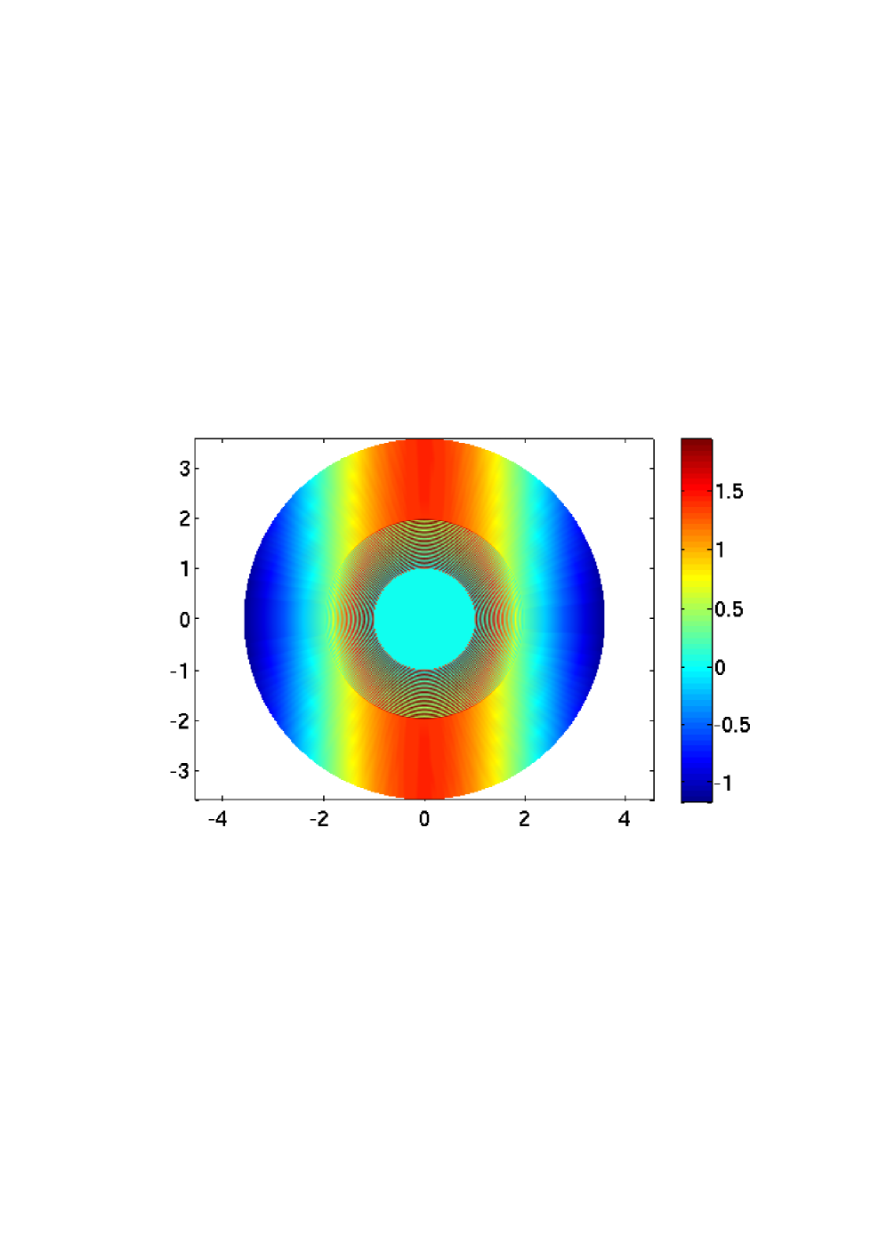
Figure 5: Plane wave and approximate cloak. Re$\,\psi$ when $E$ is not an interior Neumann eigenvalue: matter wave passes cloak almost unaltered. The Moiré pattern is an artifact.

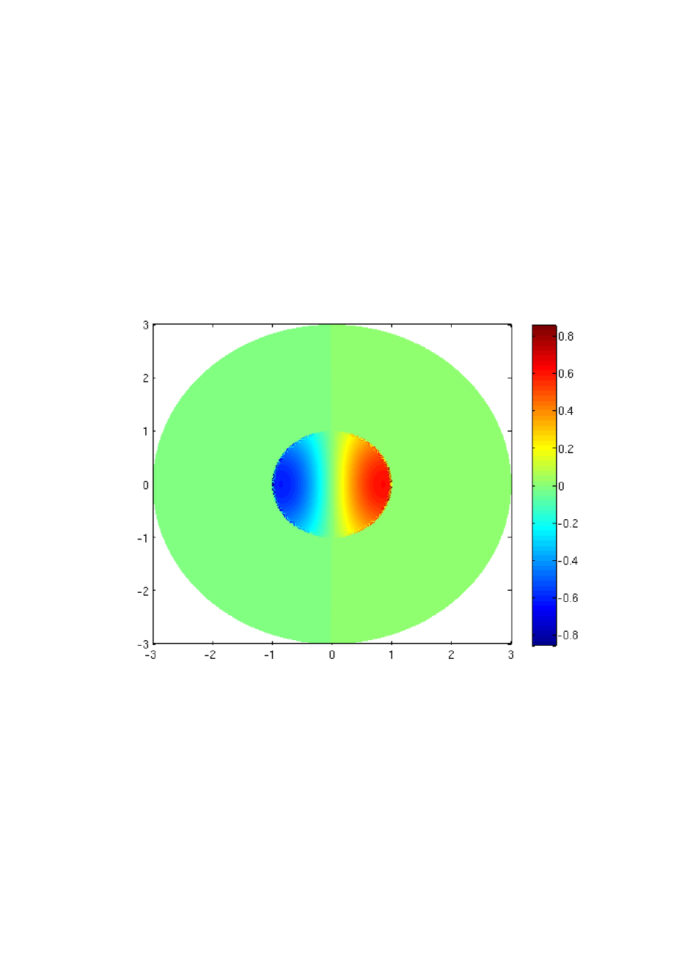
Figure 6: Almost trapped state. A noncentral almost trapped state:   Re$\,\psi$ for potential $W(x)=v_{in}\chi_{[0,0.9]}(r)$, $v_{in}=-3.92$ and $E=0.5$, surrounded by the approximate cloak described in Sec 3.5.

Assume now that $E$ is a Neumann eigenvalue of multiplicity one of the operator $-\nabla^{2}_{A}+Q$ in $B_{1}$ but is not a Dirichlet eigenvalue of operator $-\nabla^{2}_{{\widetilde{A}}}$ in $\Omega=B_{3}$. Using formulae (22)–(24), one sees that then $E$ is a eigenvalue of $D$ of multiplicity one and the corresponding eigenfunction $\phi$ is concentrated in $B_{1}$, that is, $\phi(x)=0$ for $x\in\Omega\setminus B_{1}$. Assume, for simplicity, that $\kappa=1$, and let $p$ be a function supported in $B_{1}$ that satisfies

$$a_{p}=\int_{B_{1}}\,dx\,p(x)\phi(x)=\int_{\Omega}\,dx\,g^{1/2}(x)p(x)\phi(x)\neq 0.$$

If $\Gamma$ is a contour in ${\mathbb{C}}$ around $E$ containing only one eigenvalue of $D$, then

$$\frac{1}{2\pi i}\int_{\Gamma}\,dz\,(D-z)^{-1}p=a_{p}\phi.$$ (81)

However, by (80),

$$\frac{1}{2\pi i}\int_{\Gamma}\,dz\,(D-z)^{-1}p=\lim_{n\to\infty}\frac{1}{2\pi i}\int_{\Gamma}\,dz\,(D_{n}-z)^{-1}p.$$

By standard results from spectral theory, e.g., [35], this implies that if $n$ is sufficiently large then there is only one eigenvalue $E_{n}$ of $D_{n}$ inside $\Gamma$, and $E_{n}\to E$ as $n\to\infty$. Moreover,

$$a_{p}\phi=\lim_{n\to\infty}a_{n,p}\phi_{n},$$

where $\phi_{n}$ is the eigenfunction of $D_{n}$ corresponding to the eigenvalue $E_{n}$ and $a_{n,p}$ is given as

$$a_{n,p}=\int_{\Omega}\,dx\,g_{n}^{1/2}(x)p(x)\phi_{n}(x)=\int_{B_{1}}\,dx\,p(x)\phi_{n}(x).$$

This shows, in particular, that, when $n$ is sufficiently large, the eigenfunctions $\phi_{n}$ of $D_{n}$ are close to the eigenfunction $\phi$ of $D$ and therefore are almost $0$ in $\Omega-B_{1}$.

Applying the gauge transformation (68), we see that the magnetic Schrödinger operator $-\nabla^{2}_{A}+(V_{n}^{E_{n}}+Q)$ has $E_{n}$ as an eigenvalue,

$$-\nabla^{2}_{A}\psi_{n}+(V_{n}^{E}+Q)\psi_{n}=E_{n}\psi_{n},$$

where $\psi_{n}=g_{n}(x)^{-1/2}\phi_{n}$. It follows from the above that this eigenfunction $\psi_{n}$ is close to zero outside $B_{1}$. This means that the corresponding quantum particle is mostly concentrated in $B_{1}$, which we may think of as an almost trapped state located in $B_{1}$.

4.3 Case study 3: ${\mathbb{S}}^{3}$ quantum mechanics in the lab

The basic quantum cloaking construction outlined above can be modified to make the wave function on $B_{1}$ behave (up to a small error) as though it were confined to a compact, boundaryless three-dimensional manifold which has been “glued” into the cloaked region. Mathematically, this could be any manifold, $M$, but for physical realizability, one needs to take $M$ to be the three-sphere, ${\mathbb{S}}^{3}$, topologically, but not necessarily with its standard metric, $g_{std}$. By appropriate choice of a Riemannian metric $g$ on ${\mathbb{S}}^{3}$, the resulting approximately cloaking potentials can be custom designed to support an essentially arbitrary energy level structure.

Figure 7: Schematic: Constructing an ${\mathbb{S}}^{3}$ approximate quantum cloak.

As the starting point one uses not the original cloaking conductivity $\sigma_{1}$ (the single coating construction), but instead what was referred to in [19, Sec. 2] as a double coating. This is singular (and of course anisotropic) from both sides of $\Sigma$, and in the cloaking context corresponds to coating both sides of $\Sigma$ with appropriately matched metamaterials. Here, we denote a double coating tensor by $\sigma^{(2)}$. The part of such a $\sigma^{(2)}$ inside $B_{1}$ is specified by (i) choosing a Riemannian metric $g$ on $\mathbb{S}^{3}$, with corresponding conductivity $\sigma^{ij}=|g|^{\frac{1}{2}}g^{ij}$; (ii) a small ball $\widetilde{B}_{\delta}$ about a distinguished point $x_{0}\in\mathbb{S}^{3}$; (iii) a blow-up transformation $T_{1}:\mathbb{S}^{3}-\{x_{0}\}\to\mathbb{S}^{3}-\widetilde{B}_{\delta}$ similar to the $F$ used in the standard single coating construction; and (iv) a gluing transformation $T_{2}:\mathbb{S}^{3}-\widetilde{B}_{\delta}\to B_{1}$, identifying the boundary of $\widetilde{B}_{\delta}$ with the inner edge of the cloaking surface, $\Sigma^{-}$. Then, $\sigma^{(2)}$ is defined as ${T_{2}}_{*}\left({T_{1}}_{*}\sigma\right)$ on $B_{1}$, and an appropriately matched single coating on $B_{3}-B_{1}$ as before. This correpsonds to a singular Riemannian metric $g^{(2)}$ on $B_{3}$, with a two-sided conical singularity at $\Sigma$. One can show [19, Sec. 3.3] that the finite energy distributional solutions of the Helmholtz equation $(\nabla_{g^{(2)}}+\omega^{2})u=0$ on $B_{3}$ split into direct sums of waves on $B_{3}-B_{1}$, as for $\sigma_{1}$, and waves on $B_{1}$ which are identifiable with eigenfunctions of the Laplace-Beltrami operator $-\nabla_{g}^{2}$ on the compact, boundaryless Riemannian manifold $(\mathbb{S}^{3},g)$, with eigenvalue $\omega^{2}$.

If one takes $g$ to be the standard metric on $\mathbb{S}^{3}$, then the first excited energy level is degenerate, with multiplicity 4, while a generic choice of $g$ yields all energy levels simple. On the other hand, it is known that, by suitable choice of the metric $g$, any desired finite number of energy levels and multiplicities at the bottom of the spectrum can be specified arbitrarily [12], allowing approximate quantum cloaks to be built that model abstract quantum systems, with the energy $E$ having any desired multiplicity.

References

- [1] G. Allaire: Homogenization and two-scale convergence, SIAM J. Math. Anal. 23, 1482 (1992).
- [2] G. Allaire and A. Damlamian and U. Hornung, Two-scale convergence on periodic surfaces and applications, In A. Bourgeat, C. Carasso, S. Luckhaus and A. Mikelic (eds.), Mathematical Modelling of Flow through Porous Media, 15-25, Singapore, World Scientific, 1995.
- [3] H. Attouch, Variational convergence for functions and operators, Appl. Math. Series, Pitman (Advanced Publishing Program), Boston, 1984.
- [4] A. Bensoussan, J.L. Lions and G. Papanicolaou, Asymptotic analysis for periodic structures, North-Holland, Amsterdam, 1978.
- [5] Y. Berezanskii, The uniqueness theorem in the inverse problem of spectral analysis for the Schrödinger equation (Russian), Trudy Moskov. Mat. Obsch., 7, 1 (1958).
- [6] A. Bukhgeim, Recovering a potential from Cauchy data, J. Inverse Ill-Posed Probl. 16, 19 (2008).
- [7] S. Chanillo, A problem in electrical prospection and an -dimensional Borg-Levinson theorem, Proc. Amer. Math. Soc. 108, 761 (1990).
- [8] H. Chen and C.T. Chan, Transformation media that rotate electromagnetic fields, Appl. Phys. Lett. 90, 241105 (2007).
- [9] H. Chen and C.T. Chan, Acoustic cloaking in three dimensions using acoustic metamaterials, Appl. Phys. Lett. 91, 183518 (2007).
- [10] H. Chen and C.T. Chan, Electromagnetic wave manipulation using layered systems, arXiv:0805.1328 (2008).
- [11] A. Cherkaev, Variational methods for structural optimization, Appl. Math. Sci., 140, Springer-Verlag, New York, 2000.
- [12] Y. Colin de Verdière, Construction de laplaciens dont une partie finie du spectre est donnée, Ann. Sci. École Norm. Sup. 20, 599 (1987).
- [13] D. Colton and R. Kress, Inverse Acoustic and Electromagnetic Scattering Theory,Springer-Verlag, Berlin, 1992.
- [14] S. Cummer and D. Schurig, One path to acoustic cloaking, New J. Phys. 9, 45 (2007).
- [15] S. Cummer, et al., Scattering Theory Derivation of a 3D Acoustic Cloaking Shell, Phys. Rev. Lett. 100, 024301 (2008).
- [16] G. D Maso, An Introduction to -convergence, Prog. in Nonlinear Diff. Eq. and their Appl., 8. Birkhauser Boston, Inc., Boston, 1993.
- [17] M. Farhat, S. Guenneau, A.B. Movchan and S. Enoch, Achieving invisibility over a finite range of frequencies, Optics Express, 16, 5656 (2008).
- [18] D. Gilbarg and N. Trudinger, Elliptic Partial Differential Equations of Second Order, 2nd ed., Springer-Verlag, Berlin, 1983.
- [19] A. Greenleaf, Y. Kurylev, M. Lassas, G. Uhlmann, Full-wave invisibility of active devices at all frequencies, Comm. Math. Phys., 279, 749 (2007).
- [20] A. Greenleaf, Y. Kurylev, M. Lassas, G. Uhlmann, Electromagnetic wormholes and virtual magnetic monopoles from metamaterials, Phys. Rev. Lett., 99, 183901 (2007).
- [21] A. Greenleaf, Y. Kurylev, M. Lassas, G. Uhlmann, Improvement of cylindrical cloaking with the SHS lining. Opt. Exp. 15, 12717 (2007).
- [22] A. Greenleaf, Y. Kurylev, M. Lassas, G. Uhlmann, Electromagnetic wormholes via handlebody constructions, Comm. Math. Phys., 281, 369 (2008).
- [23] A. Greenleaf, Y. Kurylev, M. Lassas, G. Uhlmann, Comment on ”Scattering Theory Derivation of a 3D Acoustic Cloaking Shell”, arXiv:0801.3279 (2008).
- [24] A. Greenleaf, Y. Kurylev, M. Lassas, G. Uhlmann, Approximate quantum and acoustic cloaking, in preparation.
- [25] A. Greenleaf, Y. Kurylev, M. Lassas, G. Uhlmann, Approximate quantum cloaking and almost trapped states, arXiv:0806.0368 (2008), submitted.
- [26] A. Greenleaf, M. Lassas, and G. Uhlmann, The Calderón problem for conormal potentials, I: Global uniqueness and reconstruction, Comm. Pure Appl. Math 56, 328 (2003).
- [27] A. Greenleaf, M. Lassas, and G. Uhlmann, Anisotropic conductivities that cannot detected by EIT, Physiolog. Meas. (special issue on Impedance Tomography), 24, 413 (2003).
- [28] A. Greenleaf, M. Lassas, and G. Uhlmann, On nonuniqueness for Calderón’s inverse problem, Math. Res. Lett. 10, 685 (2003).
- [29] P. Grinevich and R. Novikov, Transparent potentials at fixed energy in dimension two. Fixed-energy dispersion relations for the fast decaying potentials, Comm. Math. Phys. 174, 409 (1995).
- [30] S. Guenneau and F. Zolla. Homogenization of three-dimensional finite photonic crystals. Jour. of Elect. Waves and Appl., 14, 529 (2000); and Prog. In Elect. Res., 27, 91 (2000).
- [31] S. Guenneau, F. Zolla and A. Nicolet, Homogenization of three-dimensional photonic crystals with heterogeneous permittivity and permeability, Waves in Random and Complex Media, 17, 653 (2007).
- [32] A. Hendi, J. Henn, and U. Leonhardt, Ambiguities in the scattering tomography for central potentials, Phys. Rev. Lett. 97, 073902 (2006).
- [33] Y. Huang, Y. Feng and T. Jiang, Electromagnetic cloaking by layered structure of homogeneous isotropic materials, Opt. Expr., 15, 11133 (2007).
- [34] V. Jikov, S. Kozlov and O. Oleinik, Homogenization of Differential Operators, Springer-Verlag, Berlin, 1995.
- [35] T. Kato, Perturbation theory for linear operators, Springer-Verlag, New York, 1980.
- [36] R. Kohn, H. Shen, M. Vogelius and M. Weinstein, Cloaking via change of variables in electrical impedance tomography, Inverse Prob. 24, 015016 (2008).
- [37] R. Kohn, M. Vogelius, Identification of an unknown conductivity by means of measurements at the boundary, in Inverse problems (New York, 1983), SIAM-AMS Proc., 14, Amer. Math. Soc., Providence, RI, 1984
- [38] Y. Kurylev, M. Lassas and E. Somersalo, Maxwell’s equations with a polarization independent wave velocity: direct and inverse problems, Jour. Math. Pures Appl. 86 (2006), 237.
- [39] R. Lavine and A. Nachman, unpublished (1988).
- [40] U. Leonhardt, Optical conformal mapping, Science 312, 1777 (2006).
- [41] U. Leonhardt and T. Philbin, General relativity in electrical engineering, New J. Phys. 8, 247 (2006).
- [42] R. Lipton, Homogenization and field concentrations in heterogeneous media, SIAM J. Math. Anal., 38, 1048 (2006).
- [43] Y. Luo, H. Chen, J. Zhang, L. Ran and J. Kong, Design and analytically full-wave validation of the invisibility cloaks, concentrators, and field rotators created with a general class of transformations, arXiv:0712.2027 (2007).
- [44] G. Milton, The Theory of Composites, Cambridge Univ. Pr., 2001.
- [45] G. Nguetseng, A general convergence result for a functional related to the theory of homogenization, SIAM J. Math. Anal., 20, 608 (1989).
- [46] A. Norris, Acoustic cloaking theory, Proc. Roy. Soc. A, doi:10.1098/rspa.2008.0076 (2008).
- [47] J.B. Pendry, D. Schurig, and D.R. Smith, Controlling Electromagnetic Fields, Science 312, 1780 (2006).
- [48] M. Rahm, et al., Optical Design of Reflectionless Complex Media by Finite Embedded Coordinate Transformations, Phys. Rev. Lett. 100, 063903 (2008).
- [49] Z. Ruan, M. Yan, C. Neff and M. Qiu, Ideal cylindrical cloak: perfect but sensitive to tiny perturbations, Phys. Rev. Lett. 99, 113903 (2007).
- [50] D. Schurig, J. Mock, B. Justice, S. Cummer, J. Pendry, A. Starr, and D. Smith, Metamaterial electromagnetic cloak at microwave frequencies, Science 314, 977 (2006).
- [51] J. Sylvester and G. Uhlmann, A global uniqueness theorem for an inverse boundary value problem, Ann. Math. 125, 153 (1987).
- [52] A. Ward and J. Pendry, Refraction and geometry in Maxwell’s equations, J. Mod. Phys. 43, 773 (1996).
- [53] R. Weder, A rigorous analysis of high-order electromagnetic invisibility cloaks, Jour. Phys. A: Math. and Theor., 41, 065207 (2008).
- [54] S. Zhang, D. Genov, C. Sun and X. Zhang, Cloaking of matter waves, Phys. Rev. Lett. 100, 123002 (2008).
- [55] F. Zolla and S. Guenneau, Artificial ferro-magnetic anisotropy: homogenization of 3D finite photonic crystals, pp. 375-385, in Asymptotics, Singularities and Homogenization in Problems of Mechanics, Solid Mechanics and Its Applications, A.B. Movchan, ed., Kluwer Academic Pr., 2003.
- [56] F. Zolla, S. Guenneau, A. Nicholet and J. Pendry, Electromagnetic analysis of cylindrical invisibility cloaks and the mirage effect, Opt. Lett. 32, 1069 (2007).