Checking the Quality of Clinical Guidelines using Automated Reasoning Tools

Abstract

Requirements about the quality of clinical guidelines can be represented by schemata borrowed from the theory of abductive diagnosis, using temporal logic to model the time-oriented aspects expressed in a guideline. Previously, we have shown that these requirements can be verified using interactive theorem proving techniques. In this paper, we investigate how this approach can be mapped to the facilities of a resolution-based theorem prover, otter, and a complementary program that searches for finite models of first-order statements, mace-2. It is shown that the reasoning required for checking the quality of a guideline can be mapped to such fully automated theorem-proving facilities. The medical quality of an actual guideline concerning diabetes mellitus 2 is investigated in this way.

1 Introduction

Health-care is becoming more and more complicated at an astonishing rate. On the one hand, the number of different patient management options has risen considerably during the last couple of decades, whereas, on the other hand, medical doctors are expected to take decisions balancing benefits for the patient against financial costs. There is a growing trend within the medical profession to believe that clinical decision-making should be based as much as possible on sound scientific evidence; this has become known as evidence-based medicine [Woolf (2000)]. Evidence-based medicine has given a major impetus to the development of clinical guidelines, documents offering a description of steps that must be taken and considerations that must be taken into account by health-care professionals in managing a disease in a patient, to avoid substandard practices or outcomes. Their general aim is to promote standards of medical care. Clinical protocols have a similar aim as clinical guidelines, except that they offer more detail, and are often local, more detailed version of a related clinical guideline.

Researchers in artificial intelligence (AI) have picked up on these developments by designing guideline modelling languages, for instance PROforma [Fox and Das (2000)] and GLIF3 [Peleg et al. (2000)] that may be useful in developing computer-based representations of guidelines. Some of them, for example in the Asgaard project [Shahar et al. (1998)], in the CREDO project [Fox et al. (2006)] and the GLARE project [Terenziani et al. (2001), Terenziani et al. (2003)], are also involved in the design of tools that support the deployment of clinical guidelines. These languages and tools have been evolving since the 1990s, a process that is gaining momentum due to the increased interest in guidelines within the medical community. AI researchers see guidelines as good real-world examples of highly structured, systematic documents that are amenable to formalisation.

Compared to the amount of work that has been put into the formalisation of clinical guidelines, verification of guidelines has received relatively little attention. In [Shiffman and Greenes (1994)], logic was used to check whether a set of recommendations is complete, to find out whether or not the recommendations are logically consistent, and to recognise ambiguous rules if they are present. Checking the consistency of temporal scheduling constraints has also been investigated [Duftschmid et al. (2002)]. Most of the work done in the area of formal verification of clinical guidelines, i.e., proving correctness properties using formal methods, is of more recent years, e.g., as done in the Protocure project with the use of interactive theorem proving [Hommersom et al. (2007), Ten Teije et al. (2006)] and model checking [Bäumler et al. (2006), Groot et al. (2007)].

This paper explores the use of automated deduction for the verification of clinical guidelines. For the rapid development of good quality guidelines it is required that guidelines can be at least partially verified automatically; unfortunately, as of yet, there are no verification methods that can be readily used by guideline developers. Previously, it was shown that for reasoning about models of medical knowledge, for example in the context of medical expert systems [Lucas (1993)], classical automated reasoning techniques (e.g., [Robinson (1965), Wos et al. (1984)]) are a practical option. Important for the reasoning about knowledge in clinical guidelines is its temporal nature; time plays a part in the physiological mechanisms as well as in the exploration of treatment plans. As far as we know, the application of automated reasoning techniques to guideline knowledge has as yet not been investigated. The guideline we studied to this purpose has a structure similar to other guidelines and the verification principles used have sufficient generality. Thus, the results of the study go beyond the actual guideline studied.

There are two approaches to checking the quality of clinical guidelines using formal methods: (1) the object-level approach amounts to translating a guideline to a formal language, such as Asbru [Shahar et al. (1998)], and subsequently applying program verification or logical methods to analyse the resulting representation for establishing whether certain domain-specific properties hold; (2) the meta-level approach, which consists of formalising general requirements to which a guideline should comply, and then investigating whether this is the case. Here we are concerned with the meta-level approach to guideline-quality checking. For example, a good-quality clinical guideline regarding treatment of a disorder should preclude the prescription of redundant drugs, or advise against the prescription of treatment that is less effective than some alternative. An additional goal of this paper is to establish how feasible it is to implement such meta-reasoning techniques in existing tools for automated deduction for the purpose of quality checking of a clinical guideline.

Previously, we have shown that the theory of abductive diagnosis can be taken as a foundation for the formalisation of quality criteria of a clinical guideline [Lucas (2003)] and that these can be verified using (interactive) program verification techniques [Hommersom et al. (2007)]. In this paper, we provide an alternative to this approach by translating this formalism, a restricted part of temporal logic, to standard first-order logic. Furthermore, the quality criteria are interpreted in such a way that they can be stated in terms of a monotonic entailment relation. We show that, because of the restricted language needed for the formalisation of the guideline knowledge, the translation is a relatively simple fragment of first-order logic which is amended to automated verification. Thus, we show that it is indeed possible, while not easy, to cover the route from informal medical knowledge to a logical formalisation and automated verification.

The meta-level approach that is used here is particularly important for the design of clinical guidelines, because it corresponds to a type of reasoning that occurs during the guideline development process. Clearly, quality checks are useful during this process; however, the design of a guideline can be seen as a very complex process where formulation of knowledge and construction of conclusions and corresponding recommendations are intermingled. This makes it cumbersome to do interactive verification of hypotheses concerning the optimal recommendation during the construction of such a guideline, because guideline developers do not generally have the necessary background in formal methods to construct such proofs interactively. Automated theorem proving could therefore be potentially more beneficial for supporting the guideline development process.

The paper is organised as follows. In the next section, we start by explaining what clinical guidelines are, and a method for formalising guidelines by temporal logic is briefly reviewed. In Section 3 the formalisation of guideline quality using a meta-level scheme that comes from the theory of abductive diagnosis is described. The guideline on the management of diabetes mellitus type 2 that has been used in the case study is given attention in Section 4, and a formalisation of this is given as well. An approach to checking the quality of this guideline using the reasoning machinery offered by automated reasoning tools is presented in Section 5. Finally, Section 6 discusses what has been achieved, and the advantages and limitations of this approach are brought into perspective. In particular, we will discuss the role of automated reasoning in quality checking guidelines in comparison to alternative techniques such as model checking and interactive verification.

2 Framework

In this section, we review the basics about clinical guidelines and the temporal logic used in the remainder of the paper.

2.1 Clinical Guidelines

A clinical guideline is a structured document, containing detailed advice on the management of a particular disorder or group of disorders, aimed at health-care professionals. As modern guidelines are based on scientific evidence, they contain information about the quality of the evidence on which particular statements are based; e.g., statements at the highest recommendation level are usually obtained from randomised clinical trials [Woolf (2000)].

The design of a clinical guideline is far from easy. Firstly, the gathering and classification of the scientific evidence underlying and justifying the recommendations mentioned in a guideline are time consuming, and require considerable expertise of the medical field concerned. Secondly, clinical guidelines are very detailed, and making sure that all the information contained in the guideline is complete for the guideline’s purpose, and based on sound medical principles is hard work.

• Step 1: diet

• Step 2: if Quetelet Index (QI) $\leq$ 27, prescribe a sulfonylurea drug; otherwise, prescribe a biguanide drug

• Step 3: combine a sulfonylurea drug and biguanide (replace one of these by a $\alpha$-glucosidase inhibitor if side-effects occur)

• Step 4: one of the following:

  • oral anti-diabetics and insulin

  • only insulin

Figure 1: Tiny fragment of a clinical guideline on the management of diabetes mellitus type 2. If one of the steps $s$ where $s=1,2,3$ is ineffective, the management moves to step $s+1$.

An example of a part of a guideline is the following (translated) text:

1. refer to a dietist; check blood glucose after 3 months
2. in case (1) fails and Quetelet Index (QI) $\leq$ 27, then administer a sulfonylureum derivate (e.g. tolbutamide, 500 mg 1 time per day, max. 1000 mg 2 per day) and in case of Quetelet Index (QI) $>$ 27 biguanide (500 mg 1 per day, max. 1000 mg 3 times per day); start with lowest dosage, increase each 2-4 weeks if necessary

It is part of a real-world guideline for general practitioners about the treatment of diabetes mellitus type 2. Part of this description includes details about dosage of drugs at specific time periods. As we want to reason about the general structure of the guideline, rather than about dosages or specific time periods, we have made an abstraction as shown in Fig. 1. This guideline fragment is used in this paper as a running example.

Guidelines can be as large as 100 pages; however, the number of recommendations they include are typically few. In complicated diseases, each type of disease is typically described in different sections of a guideline, which provides ways to modularise the formalisation in a natural fashion. For example, in the Protocure project, we have formalised an extensive guideline about breast cancer treatment, which includes recommendations very similar in nature and structure to the abstraction shown in Fig. 1. In this sense, the fragment in Fig. 1 can be lookup upon as one of the recommendations in any guideline whatever its size. Clinical protocols are normally more detailed, and the abstraction used here will not be appropriate if one wishes to consider such details in the verification process. For example, in the Protocure project we also carried out work on the verification of a clinical protocol about the management of neonatal jaundice, where we focussed on the levels of a substance in the blood (bilirubin) [Ten Teije et al. (2006)]. Clearly, in this case abstracting away from substance levels would be inappropriate.

The conclusions that can be reached by the rest of the paper are relative to the abstraction that was chosen. The logical methods that we employ are related to this level of abstraction, even though other logical methods are available to deal issues such as more detailed temporal reasoning [Moszkowski (1985)] or probabilities [Richardson and Domingos (2006), Kersting and De Raedt (2000)], which might be necessary for some guidelines or protocols. Nonetheless, where development of an abstraction of a medical document will be necessary for any verification task, the way it is done is dependent on what is being verified and the nature of the document. The level of abstraction that we employ allow us to reason about the structure and effects of treatments, which, in our view, is the most important aspect of many guidelines.

One way to use formal methods in the context of guidelines is to automatically verify whether or not a clinical guideline fulfils particular properties, such as whether it complies with quality indicators as proposed by health-care professionals [Marcos et al. (2002)]. For example, using particular patient assumptions such as that after treatment the levels of a substance are dangerously high or low, it is possible to check whether this situation does or does not violate the guideline. However, verifying the effects of treatment as well as examining whether a developed clinical guideline complies with global criteria, such as that it avoids the prescription of redundant drugs, or the request of tests that are superfluous, is difficult to impossible if only the guideline text is available. Thus, the capability to check whether a guideline fulfils particular medical objectives may require the availability of more medical knowledge than is actually specified in a clinical guideline. How much additional knowledge is required may vary from guideline to guideline. In the development of the theory below it is assumed that at least some medical background knowledge is required; the extent and the purpose of that background knowledge is subsequently established using the diabetes mellitus type 2 guideline. The development, logical implementation, and evaluation of a formal method that supports this process is the topic of the remainder of the paper.

2.2 Using Temporal Logic in Clinical Guidelines

Table 1: Used temporal operators; $t$ stands for a time instance.

Notation	Informal meaning	Formal meaning
$\textsf{H}\varphi$	$\varphi$ has always been true in the past	$t\vDash\textsf{H}\varphi$ iff $\forall t^{\prime}<t:t^{\prime}\vDash\varphi$
$\varphi\,\textsf{U}\,\psi$	$\varphi$ is true until $\psi$ holds	$\vDash\varphi\,\textsf{U}\,\psi$ iff $\exists t^{\prime}\geq t:t^{\prime}\vDash\psi$
		$\textup{and }\forall t^{\prime\prime}:t\leq t^{\prime\prime}<t^{\prime}\rightarrow t^{\prime\prime}\vDash\varphi$

Many representation languages for formalising and reasoning about medical knowledge have been proposed, e.g., predicate logic [Lucas (1993)], (heuristic) rule-based systems [Shortliffe (1974)], and causal representations [Patil (1981)]. It is not uncommon to abstract from time in these representations; however, as medical management is very much a time-oriented process, guidelines should be looked upon in a temporal setting. It has been shown previously that the step-wise, possibly iterative, execution of a guideline, such as the example in Fig. 1, can be described precisely by means of temporal logic [Ten Teije et al. (2006)]. In a more practical setting it is useful to support the modelling process by means of tools. There is promising research for maintaining a logical knowledge base in the context of the semantic web (e.g., the Protégé-OWL editor), and the logical formalisation described in this paper could profit from the availability of such tools.

The temporal logic that we use here is a modal logic, where relationships between worlds in the usual possible-world semantics of modal logic is understood as time order, i.e., formulae are interpreted in a temporal frame ${\mathcal{}F}=({\mathbb{T}},<,I)$, where ${\mathbb{T}}$ is the set of intervals or time points, $<$ a time ordering, and $I$ an interpretation of the language elements with respect to ${\mathbb{T}}$ and $<$. The language of first-order logic, with equality and unique names assumption, is augmented with the operators U, H, G, P, and F, where the temporal semantics of the first two operators is defined in Table 1. The last four operators are simply defined in terms of the first two operators:

$$\begin{array}[]{lr}\vDash\textsf{P}\varphi\leftrightarrow\neg\textsf{H}\neg\varphi&\mbox{(somewhere in the past)}\\ \vDash\textsf{F}\varphi\leftrightarrow\top\textsf{U}\varphi&\mbox{(now or somewhere in the future)}\\ \vDash\textsf{G}\varphi\leftrightarrow\neg\textsf{F}\neg\varphi&\mbox{(now and always in the future)}\end{array}$$

This logic offers the right abstraction level to cope with the nature of the temporal knowledge in clinical guidelines required for our purposes.

Other modal operators added to the language of first-order logic include X, where $\textsf{X}\varphi$ has the operational meaning of an execution step, followed by execution of program part $\varphi$. Even though this operator is not explicitly used in our formalisation of medical knowledge, a principle similar to the semantics of this operator is used in Section 5.5 for reasoning about the step-wise execution of the guideline.

In addition, axioms can be added that indicate that progression in time is linear (there are other possible axiomatisations, such as branching time, see [Turner (1985)]). The most important of these are:

• Transitivity: $\vDash\textsf{F}\textsf{F}\varphi\rightarrow\textsf{F}\varphi$

• Backward linearity: $\vDash(\textsf{P}\varphi\wedge\textsf{P}\psi)\rightarrow(\textsf{P}(\varphi\wedge\psi)\vee\textsf{P}(\varphi\wedge\textsf{P}\psi)\vee\textsf{P}(\textsf{P}\varphi\wedge\psi))$

• Forward linearity: $\vDash(\textsf{F}\varphi\wedge\textsf{F}\psi)\rightarrow(\textsf{F}(\varphi\wedge\psi)\vee\textsf{F}(\varphi\wedge\textsf{F}\psi)\vee\textsf{F}(\textsf{F}\varphi\wedge\psi))$

Transitivity ensures that we can move along the time axis from the past into the future; backward and forward linearity ensure that the time axis does not branch. Consider, for example, axiom (3), which says that if there exists a time $t$ when $\varphi$ is true, and a time $t^{\prime}$ when $\psi$ holds, then there are three possibilities: $\varphi$ and $\psi$ hold at the same time, or at some time in the future $\varphi$ and further away in the future $\psi$ hold; the meaning of the last disjunct is similar. Other useful axioms concern the boundedness of time; assuming that time has no beginning and no end, gives rise to the following axioms: $\vDash\textsf{H}\varphi\rightarrow\textsf{P}\varphi$ and $\vDash\textsf{G}\varphi\rightarrow\textsf{F}\varphi$.

Alternative formal languages for modelling medical knowledge are possible. For example, differential equations describing compartmental models that are used to predict changes in physiological variables in individual patients have been shown to be useful (e.g., [Magni et al. (2000), Lehmann (1998)]). In the context of clinical reasoning they are less useful, as they essentially concern levels of substances as a function of time and, thus, do not offer the right level of abstraction that we are after.

3 Application to Medical Knowledge

It is well-known that knowledge elicitation is difficult (see e.g., [Evans (1988)]) and due to complexity and uncertainty this is particularly true for medical knowledge (see e.g., [van Bemmel and Musen (2002)]). The effort to acquire this knowledge is dependent on the availability of the knowledge in the guideline and the complexity of the mechanisms that are involved in the development of the disease. For evidence-based guidelines, a large part of the relevant knowledge required for checking the quality of the recommendations is included in the guideline, which makes the problem more contained than the problem of arbitrary medical knowledge elicitation.

The purpose of a clinical guideline is to have a certain positive effect on the health status of a patient to which the guideline applies. To establish that this is indeed the case, knowledge concerning the normal physiology and abnormal, disease-related pathophysiology of a patient is required. Some of this physiological knowledge may be missing from the clinical guidelines; however, much of this knowledge can be acquired from textbooks on medical physiology, which reduces the amount of effort required to construct such knowledge models. The latter approach was taken in this research.

It is assumed that two types of knowledge are involved in detecting the violation of good medical practice:

• Knowledge concerning the (patho)physiological mechanisms underlying the disease, and the way treatment influences these mechanisms. The knowledge involved could be causal in nature, and is an example of object-knowledge.

• Knowledge concerning good practice in treatment selection; this is meta-knowledge.

Below we present some ideas on how such knowledge may be formalised using temporal logic (cf. [Lucas (1995)] for earlier work in the area of formal modelling of medical knowledge).

We are interested in the prescription of drugs, taking into account their mode of action. Abstracting from the dynamics of their pharmacokinetics, this can be formalised in logic as follows:

$$(\textsf{G}\,d\wedge r)\rightarrow\textsf{G}(m_{1}\wedge\cdots\wedge m_{n})$$ (1)

where $d$ is the name of a drug, $r$ is a (possibly negative or empty) requirement for the drug to take effect, and $m_{k}$ is a mode of action, such as decrease of release of glucose from the liver, which holds at all future times. Note that we assume that drugs are applied for a long period of time, here formalised as ‘always’. This is reasonable if we think of the models as finite structures that describe a somewhat longer period of time, allowing the drugs to take effect. Synergistic effects and interactions amongst drugs can also be formalised along those lines, as required by the guideline under consideration. This can be done either by combining their joint mode of action, by replacing $d$ in the formula above by a conjunction of drugs, by defining harmful joint effects of drugs in terms of inconsistency, or by reasoning about modes of actions. As we do not require this feature for the clinical guideline considered in this paper, we will not go into details. In addition, it is possible to reason about such effects using special purpose temporal logics with abstraction and constraints, such as developed by Allen [Allen (1983)] and Terenziani [Terenziani (2000)] without a connection to a specific field, and by Shahar [Shahar (1997)] for the field of medicine. Thus, temporal logics are expressive enough to cope with extensions to the formalisation as used in this paper.

The modes of action $m_{k}$ can be combined, together with an intention $n$ (achieving normoglycaemia, i.e., normal blood glucose levels, for example), a particular patient condition $c$, and requirements $r_{j}$ for the modes of action to be effective:

$$(\textsf{G}m_{i_{1}}\wedge\cdots\wedge\textsf{G}m_{i_{m}}\wedge r_{1}\wedge\cdots\wedge r_{p}\wedge\textsf{H}c)\rightarrow\textsf{G}n$$ (2)

For example, if the mode describes that there is a stimulus to secrete more insulin and the requirement that sufficient capacity to provide this insulin is fulfilled, then the amount of glucose in the blood will decrease.

Good practice medicine can then be formalised as follows. Let ${\mathcal{}B}$ be background knowledge, $T\subseteq\{d_{1},\ldots,d_{p}\}$ be a set of drugs, $C$ a collection of patient conditions, $R$ a collection of requirements and $N$ a collection of intentions which the physician has to achieve. As an abbreviation, the union of $C$ and $R$, i.e., the variables describing the patient, will be referred to as $P$, i.e., $P=C\cup R$. Finding an acceptable treatment given such knowledge amounts to finding an explanation, in terms of a treatment, that the intention will be achieved. Finding the best possible explanation given a number of findings is called abductive reasoning [Console and Torasso (1991), Poole (1990)]. We say that a set of drugs $T$ is a treatment according to the theory of abductive reasoning if [Lucas (2003)]:

(M1)

${\mathcal{}B}\cup\textsf{G}T\cup P\nvDash\bot$ (the drugs do not have contradictory effects), and

(M2)

${\mathcal{}B}\cup\textsf{G}T\cup P\vDash N$ (the drugs handle all the patient problems intended to be managed).

One could think of the formula ${\mathcal{}B}\cup\textsf{G}T\cup P$ as simulating a particular patient $P$ given a particular treatment $T$. For each relevant patient groups, these properties can be investigated. If in addition to (M1) and (M2) condition

(M3)

$O_{\varphi}(T)$ holds, where $O_{\varphi}$ is a meta-predicate standing for an optimality criterion or combination of optimality criteria $\varphi$, then the treatment is said to be in accordance with good-practice medicine.

A typical example of this is subset minimality $O_{\subset}$:

$$O_{\subset}(T)\equiv\forall T^{\prime}\subset T:T^{\prime}\;\mbox{is not a treatment according to {(M1)} and {(M2)}}$$ (3)

i.e., the minimum number of effective drugs are being prescribed. For example, if $\{d_{1},d_{2},d_{3}\}$ is a treatment that satisfies condition (M3) in addition to (M1) and (M2), then the subsets $\{d_{1},d_{2}\}$, $\{d_{2},d_{3}\}$, $\{d_{1}\}$, and so on, do not satisfy conditions (M1) and (M2). In the context of abductive reasoning, subset minimality is often used in order to distinguish between various solutions; it is also referred to in literature as Occam’s razor. Another definition of the meta-predicate $O_{\varphi}$ is in terms of minimal cost $O_{c}$:

$$O_{c}(T)\equiv\forall T^{\prime},\mbox{with}\;T^{\prime}\;\mbox{a treatment:}\;\;c(T^{\prime})\geq c(T)$$ (4)

where $c(T)=\sum_{d\in T}\textit{cost}(d)$; combining the two definitions also makes sense. For example, one could come up with a definition of $O_{\subset,c}$ that among two subset-minimal treatments selects the one that is the cheapest in financial or ethical sense.

The quality criteria that we have presented in this section could also be taken as starting points for critiquing, i.e., criticising clinical actions performed and recorded by a physician (cf. [Miller (1984)] for an early critiquing system), especially if we consider the formalisation of the background knowledge a model for simulating a patient receiving a specific treatment. However, here we look for means to criticise the recommendations given by the guidelines.

In order to verify the quality of guidelines, we do not make use of data from medical records. The use of such data is especially important if one wishes to empirically evaluate the guideline. As data may be missing from the database—a very common situation in clinical datasets—tests ordered for a patient and treatments given to the patient may not be according to the guideline. Therefore, such datasets cannot be used to identify problems with the clinical guideline. Results would tell as much about the dataset as about the guidelines. Once the guideline has been shown to be without flaws, it becomes interesting to carry out subsequent evaluation of the guideline using patient data. These were the main reasons why we explored guideline quality by using well-understood and well-described data from hypothetical patients; this simulates the way medical doctors would normally critically look at a guideline. Notice the similarity with use-cases in software engineering. This method is practical and possible, and could be used in the process of designing a guideline.

4 Management of Diabetes Mellitus Type 2

To determine the global quality of the guideline, the background knowledge itself was only formalised so far as required for investigating the usefulness of the theory of quality checking introduced above. The knowledge that is presented here was acquired with the help of a physician, though this knowledge can be found in many standard textbooks on physiology (e.g., [Ganong (2005), Guyton and Hall (2000)]).

4.1 Initial Analysis

It is well known that diabetes type 2 is a very complicated disease: various metabolic control mechanisms are deranged and many different organ systems, such as the cardiovascular and renal system, may be affected by the disorder. Here we focus on the derangement of glucose metabolism in diabetic patients, and even that is nontrivial. To support non-expert medical doctors in the management of this complicated disease in patients, access to a guideline is really essential.

One would expect that as this disorder is so complicated, the diabetes mellitus type 2 guideline is also complicated. This, however, is not the case, as may already be apparent from the guideline fragment shown in Fig. 1. This indicates that much of the knowledge concerning diabetes mellitus type 2 is missing from the guideline, and that without this background knowledge it will be impossible to spot the sort of flaws we are after. Hence, the conclusion is that a deeper analysis is required; the results of such an analysis are discussed next.

4.2 Diabetes Type 2 Background Knowledge

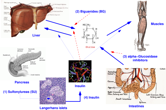
Figure 2: Summary of drugs and mechanisms controlling the blood level of glucose; $-$ $-$ $\rightarrow$: inhibition, $\cdots\cdots$$\rightarrow$: stimulation.

Fig. 2 summarises the most important mechanisms and drugs involved in the control of the blood level of glucose. The protein hormone insulin, which is produced by the B cells in the Langerhans islets of the pancreas, has the following major effects:

• it increases the uptake of glucose by the liver, where it is stored as glycogen, and inhibits the release of glucose from the liver;

• it increases the uptake of glucose by insulin-dependent tissues, such as muscle and adipose tissue.

At some stage in the natural history of diabetes mellitus type 2, the level of glucose in the blood is too high (hyperglycaemia) due to decreased production of insulin by the B cells. A popular hypothesis explaining this phenomenon is that target cells have become insulin resistant, which with a delay causes the production of insulin by the B cells to raise. After some time, the B cells become exhausted, and they are no longer capable of meeting the demands for insulin. As a consequence, hyperglycaemia develops.

Treatment of diabetes type 2 consists of:

• Use of sulfonylurea (SU) drugs, such as tolbutamid. These drugs stimulate the B cells in producing more insulin, and if the cells are not completely exhausted, the hyperglycaemia can thus be reverted to normoglycaemia (normal blood glucose levels).

• Use of biguanides (BG), such as metformin. These drugs inhibit the release of glucose from the liver.

• Use of $\alpha$-glucosidase inhibitors. These drugs inhibit (or delay) the absorption of glucose from the intestines.

• Injection of insulin. This is the ultimate, causal treatment.

As insulin is typically administered by injection, in contrast to the other drugs which are normally taken orally, doctors prefer to delay prescribing insulin as long as possible. Thus, the treatment part of the diabetes type 2 guideline mentions that one should start with prescribing oral antidiabetics (SU or BG, cf. Fig. 1). Two of these can also be combined if taking only one has insufficient glucose-level lowering effect. If treatment is still unsatisfactory, the guideline suggests to: (1) either add insulin, or (2) stop with the oral antidiabetics entirely and to start with insulin.

From a medical point of view, advice (1) above is somewhat curious. If the oral antidiabetics are no longer effective enough, the B cells could be completely exhausted. Under these circumstances, it does not make a lot of sense to prescribe an SU drug. The guideline here assumes that the B cells are always somewhat active, which may limit the amount of insulin that has to be prescribed. Similarly, prescription of a BG (or a $\alpha$-glucosidase inhibitor) is justified, as by adding such an oral antidiabetic to insulin, the number of necessary injections can be reduced from twice a day to once a day. It should be noted that, when on insulin treatment, patients run the risk of getting hypoglycaemia, which is a side effect of insulin treatment not mentioned explicitly in the guideline.

The background knowledge concerning the (patho-)physiology of the glucose metabolism as described above is formalised using temporal logic, and kept as simple as possible. The specification is denoted by ${\mathcal{}B}_{\mbox{\scriptsize DM2}}$:

(1)	$\textsf{G}\,\textrm{Drug}(\textit{insulin})\rightarrow\textsf{G}($	$\textit{uptake}(\textit{liver},\textit{glucose})=\textit{up}\;\wedge$
		$\textit{uptake}(\textit{peripheral-tissues},\textit{glucose})=\textit{up})$
(2) $\textsf{G}(\textit{uptake}(\textit{liver},\textit{glucose})=\textit{up}\rightarrow\textit{release}(\textit{liver},\textit{glucose})=\textit{down})$
(3) $(\textsf{G}\,\textrm{Drug}(\textrm{SU})\wedge\neg\textit{capacity}(\textit{b-cells},\textit{insulin})=\textit{exhausted})$
	$\rightarrow\textsf{G}\textit{secretion}(\textit{b-cells},\textit{insulin})=\textit{up}$
(4) $\textsf{G}\,\textrm{Drug}(\textrm{BG})\rightarrow\textsf{G}\textit{release}(\textit{liver},\textit{glucose})=\textit{down}$
(5)	$($	$\textsf{G}\textit{secretion}(\textit{b-cells},\textit{insulin})=\textit{up}\;\wedge$ $\textit{capacity}(\textit{b-cells},\textit{insulin})=\textit{subnormal}\;\wedge$
		$\textrm{QI}\leq 27\wedge\textsf{H}\,\textrm{Condition}(\textit{hyperglycaemia}))$ $\rightarrow\textsf{G}\,\textrm{Condition}(\textit{normoglycaemia})$
(6) $(\textsf{G}\textit{release}(\textit{liver},\textit{glucose})=\textit{down}\;\wedge$ $\textit{capacity}(\textit{b-cells},\textit{insulin})=\textit{subnormal}\;\wedge$
		$\textrm{QI}>27\wedge\textsf{H}\,\textrm{Condition}(\textit{hyperglycaemia}))$ $\rightarrow\textsf{G}\,\textrm{Condition}(\textit{normoglycaemia})$
(7)	$($	$($	$\textsf{G}\textit{release}(\textit{liver},\textit{glucose})=\textit{down}\;\vee$ $\textsf{G}\textit{uptake}(\textit{peripheral-tissues},\textit{glucose})=\textit{up})\;\wedge$
		$\textit{capacity}(\textit{b-cells},\textit{insulin})=\textit{nearly-exhausted}\;\wedge$ $\textsf{G}\textit{secretion}(\textit{b-cells},\textit{insulin})=\textit{up}\;\wedge$
		$\textsf{H}\,\textrm{Condition}(\textit{hyperglycaemia}))$ $\rightarrow\textsf{G}\,\textrm{Condition}(\textit{normoglycaemia})$
(8) $(\textsf{G}\textit{uptake}(\textit{liver},\textit{glucose})=\textit{up}\;\wedge$ $\textsf{G}\textit{uptake}(\textit{peripheral-tissues},\textit{glucose})=\textit{up})\;\wedge$
		$\textit{capacity}(\textit{b-cells},\textit{insulin})=\textit{exhausted}\;\wedge$ $\textsf{H}\,\textrm{Condition}(\textit{hyperglycaemia}))$
	$\rightarrow\textsf{G}(\textrm{Condition}(\textit{normoglycaemia})\vee\textrm{Condition}(\textit{hypoglycaemia}))$
(9) $(\textrm{Condition}(\textit{normoglycaemia})$ $\oplus$ $\textrm{Condition}(\textit{hypoglycaemia})$ $\oplus$
		$\textrm{Condition}(\textit{hyperglycaemia}))$	$\land$ $\neg(\textrm{Condition}(\textit{normoglycaemia})$	$\land$
		$\textrm{Condition}(\textit{hypoglycaemia})$ $\land$ $\textrm{Condition}(\textit{hyperglycaemia}))$

where $\oplus$ stands for the exclusive OR. Note that when the B cells are exhausted, increased uptake of glucose by the tissues may result not only in normoglycaemia but also in hypoglycaemia. Note that this background knowledge was originally developed for reasoning about the application of a single treatment. It requires some modification in order to reason about the whole guideline fragment (see Section 5.5).

4.3 Quality Check

The consequences of various treatment options can be examined using the method introduced in Section 3. Hypothetical patients for whom it is the intention to reach a normal level of glucose in the blood (normoglycaemia) and one of the steps in the guideline is applicable in the guideline fragment given in Fig. 1, are considered, for example:

• Consider a patient with hyperglycaemia due to nearly exhausted B cells. For these patients, the third step of Fig. 1 is applicable, so we check that:

$$\begin{array}[]{l}{\mathcal{}B}_{\mbox{\scriptsize DM2}}\cup\textsf{G}\,T\cup\{\textit{capacity}(\textit{b-cells},\textit{insulin})=\textit{nearly-exhausted}\}\;\cup\\[4.30554pt] \;\;\;\;\;\{\textsf{H}\,\textrm{Condition}(\textit{hyperglycaemia})\}\vDash\textsf{G}\,\textrm{Condition}(\textit{normoglycaemia})\end{array}$$

holds for $T=\{\textrm{Drug}(\textrm{SU}),\textrm{Drug}(\textrm{BG})\}$, which also satisfies the minimality condition $O_{\subset}(T)$.

• Prescription of treatment $T=\{\textrm{Drug}(\textrm{SU}),\textrm{Drug}(\textrm{BG}),\textrm{Drug}(\textrm{insulin})\}$ for a patient with exhausted B cells, for which the intended treatment regime is described in the fourth step of Fig. 1, yields:

$$\begin{array}[]{l}{\mathcal{}B}_{\mbox{\scriptsize DM2}}\cup\textsf{G}\,T\cup\{\textit{capacity}(\textit{b-cells},\textit{insulin})=\textit{exhausted}\}\;\cup\\[4.30554pt] \;\;\;\;\{\textsf{H}\,\textrm{Condition}(\textit{hyperglycaemia})\}\vDash\\[4.30554pt] \;\;\;\;\;\;\;\;\textsf{G}(\textrm{Condition}(\textit{normoglycaemia})\vee\textrm{Condition}(\textit{hypoglycaemia}))\end{array}$$

In the last case, it appears that it is possible that a patient develops hypoglycaemia due to treatment; if this possibility is excluded from axiom (8) in the background knowledge, then the minimality condition $O_{\subset}(T)$, and also $O_{c}(T)$, does not hold since insulin by itself is enough to reach normoglycaemia. In either case, good practice medicine is violated, which is to prescribe as few drugs as possible, taking into account costs and side-effects of drugs. Here, three drugs are prescribed whereas only two should have been prescribed (BG and insulin, assuming that insulin alone is too costly), and the possible occurrence of hypoglycaemia should have been prevented.

5 Automated Quality Checking

Figure 3: Translation of medical knowledge.

As mentioned in the introduction, we have explored the feasibility of using automated reasoning tools to check the quality of guidelines, in the sense described above.

5.1 Motivation for using Automated Reasoning

Several techniques are available for reasoning with temporal logic. Firstly, an automated theorem prover aims at proving theorems without any interaction from the user. This is a problem with high complexity; e.g., for first-order logic, this problem is recursively enumerable. For this reason, interactive theorem proving has been used as an alternative, where it is possible and sometimes necessary to give hints to the system. As a consequence, more complicated problems can be handled; however, in the worst case every step of the proof has to be performed manually.

For our work, it is of interest to obtain insight how much of the proof effort can be automated as this would clearly improve the practical usefulness of employing formal methods in the process of guideline development. In our previous work we have considered using interactive theorem proving [Hommersom et al. (2007)]. This was a successful experiment; however, the number of interactions that were needed were still high and a lot of expertise in the area of theorem proving is required for carrying out this task. Furthermore, there has been considerable progress in terms of speed and the size of problems that theorem provers can handle [Pelletier et al. (2002)]. In our opinion, these developments provide enough justification to explore the use of automated reasoning techniques in combination with specific strategies.

One of the most important application areas of model finders and theorem provers is program verification. In programs there is a clear beginning of the execution, which makes it intuitive to think about properties that occur after the start of the program. Therefore, it is not surprising that much work that has been done in the context of model finding and theorem proving only deals with the future time modality. However, it is more natural to model medical knowledge with past time operators, i.e., what happened to the patient in the past. It is well-known that formulas with a past-time modality can be mapped to a logical formula with only future time modalities such that both formulas are equivalent for some initial state [Gabbay (1989)]. The main drawback of this approach is that formulas will get much larger in size [Markey (2003)] and as a consequence become much harder to verify in a theorem prover designed for modal logics.

For this reason, we have chosen to use an alternative approach which uses a relational translation to map the temporal logic formulas to first-order logic. As primary tools we used the resolution-based theorem prover otter [McCune (2003)] and the finite model searcher mace-2 [McCune (2001)], which take first-order logic with equality as their input. These systems have been optimised for reasoning with first-order logical formulas and offer various reasoning strategies to do this efficiently. For example, otter offers the set-of-support strategy and hyperresolution as efficient reasoning methods. There are alternative systems that could have been used; however, it is not the aim of this paper to compare these systems. otter has been proven to be robust and efficient, and has been successfully applied to solve problems of high complexity, for example in the area of algebra [Phillips and Vojtěchovskiý (2005)] and logic [Jech (1995)].

There has been work done to improve the speed of resolution-based theorem provers on modal formulas [Areces et al. (2000)], but again, converse modalities such as the past-time operators are not considered. We found that the general heuristics applicable to full first-order logic are sufficient to our task.

5.2 Translation

In order to prove meta-level properties, it is necessary to reason at the object-level. Object-level properties typically do not contain background knowledge concerning the validity what it being verified. For example, the (M2) property of Section 3 has a clear meaning in terms of clinical guidelines, which would be lost if stated as an object-level property. Moreover, it is not (directly) possible to state that something does not follow at the object level. Fig. 3 summarises the general approach. We will first give a definition for translating the object knowledge to standard logic and then the translation of the meta-level knowledge will follow.

5.2.1 Translation of Object Knowledge

The background knowledge, as defined in Subsection 4.2, is translated into first order logic. For every function $f$ with two elements in the co-domain, call these $\{c_{1},c_{2}\}$, we introduce a fresh variable $p$ for every element $a$ in the domain such that $f(a)=c_{1}$ holds iff $p$ holds, and $f(a)=c_{2}$ holds iff $\neg p$ holds. For example, axiom (2) of $\mathcal{B}_{DM2}$ in Section 4.2 is represented by defining ‘$\textit{uptake}(\textit{liver},\textit{glucose})=\textit{up}$’ and ‘$\textit{release}(\textit{liver},\textit{glucose})=\textit{up})$’ as propositions and rewriting this axiom as:

$$\textsf{G}(`\textit{uptake}(\textit{liver},\textit{glucose})=\textit{up}\mbox{'}\rightarrow\neg(`\textit{release}(\textit{liver},\textit{glucose})=\textit{up}\mbox{'}))$$

For the capacity function, a function with three elements in its co-domain, we add a proposition $p_{x}$ for each expression $\textit{capacity}(\textit{b-cells},\textit{insulin})=x$ and an axiom saying that each pair of these propositions are mutually exclusive. Finally, the term $\textrm{QI}>27$ is interpreted as a proposition as well, i.e., we do not reason about the numerical value of QI.

Technically, this translation is not required, since we could extend the translation below to full first-order temporal logic. In practice however, we would like to avoid additional complexity from first-order formulas during the automated reasoning.

The relational translation (e.g., [Moore (1979), Areces et al. (2000), Schmidt and Hustadt (2003)]) $\textup{{ST}}_{t}(\varphi)$, also referred to as the standard translation, translates a propositional temporal logical formula $\varphi$ into a formula in a first-order logic with (time-indexed) unary predicate symbols $P$ for every propositional variable $p$ and one binary predicate $>$. It is defined as follows, where $t$ is an individual variable standing for time:

$$\begin{array}[]{lll}\textup{{ST}}_{t}(p)&\textup{iff}&P(t)\\ \textup{{ST}}_{t}(\neg\varphi)&\textup{iff}&\neg\textup{{ST}}_{t}(\varphi)\\ \textup{{ST}}_{t}(\varphi\land\psi)&\textup{iff}&\textup{{ST}}_{t}(\varphi)\land\textup{{ST}}_{t}(\psi)\\ \textup{{ST}}_{t}(\textsf{G}\varphi)&\textup{iff}&\forall t^{\prime}\;(t\not>t^{\prime}\rightarrow\textup{{ST}}_{t^{\prime}}(\varphi))\\ \textup{{ST}}_{t}(\textsf{H}\varphi)&\textup{iff}&\forall t^{\prime}\;(t>t^{\prime}\rightarrow\textup{{ST}}_{t^{\prime}}(\varphi))\\ \end{array}$$

Note that the last two elements of the definition give the meaning of the G modality and its converse, the H modality. For example, the formula $\textsf{G}(p\rightarrow\textsf{P}p)$ translates to $\forall t_{2}\;(t\not>t_{2}\rightarrow(P(t_{2})\rightarrow\exists t_{3}\;(t_{2}>t_{3}\land P(t_{3})))$. It is straightforward to show that a formula in temporal logic is satisfiable if and only if its relational translation is. Also, recall that we use set union to denote conjunction, thus $\textup{{ST}}_{t}(\Gamma\cup\Delta)$ is defined as $\textup{{ST}}_{t}(\Gamma)\land\textup{{ST}}_{t}(\Delta)$.

In the literature a functional approach to translating modal logic has appeared as well [Ohlbach (1988)], which relies on a non-standard interpretation of modal logic and could be taken as an alternative to this translation.

5.2.2 Translation of Meta-level Knowledge

Again, we consider the criteria for good practice medicine and make them suitable for use with the automated reasoning tools. In order to stress that we deal with provability in these tools, we use the ‘$\vdash$’ symbol instead of the ‘$\models$’ (validity) symbol. We say that a treatment $T$ is a treatment complying with the requirements of good practice medicine iff:

(M1^′)

$\textup{{ST}}_{t}(\mathcal{B}\cup\textsf{G}T\cup C\cup R)\nvdash\bot$

(M2^′)

$\textup{{ST}}_{t}(\mathcal{B}\cup\textsf{G}T\cup C\cup R\cup\neg N)\vdash\bot$

(M3^′)

$\forall T^{\prime}\subset T:T^{\prime}\;\mbox{is not a treatment according to {(M1${}^{\prime}$)} and {(M2${}^{\prime}$)}}$

Criterion (M3^′) is a specific instance of (M3), i.e., subset minimality as explained in Section 3 (Equation (3)). As the relational translation preserves satisfiability, these quality requirements are equivalent to their unprimed counterparts in Section 3. To automate this reasoning process we use mace-2 to verify (M1^′), otter to verify (M2^′), and (M3^′) can be seen as a combination of both for all subsets of the given treatment.

5.3 Results

In this subsection we will discuss the actual implementation in otter and some results obtained by using particular heuristics.

5.3.1 Resolution Strategies

An advantage that one gains from using a standard theorem prover that a whole range of different resolution rules and search strategies are available and can be varied depending on the problem. otter uses the set-of-support strategy [Wos et al. (1965)] as a standard strategy. In this strategy the original set of clauses is divided into a set-of-support and a usable set such that in every resolution step at least one of the parent clauses has to be member of the set-of-support and each resulting resolvent is added to the set-of-support.

Looking at the structure of the formulas in Section 4, one can see that formulas are of the form $p_{0}\wedge\cdots\wedge p_{n}\rightarrow q$, where $p_{0}\wedge\cdots\wedge p_{n}$ and $q$ are almost all positive literals. Hence, we expect the occurrence of mainly negative literals in our clauses, which can be exploited by using negative hyperresolution (neg_hyper for short) [Robinson (1965)] in otter. With this strategy a clause with at least one positive literal is resolved with one or more clauses only containing negative literals (i.e., negative clauses), provided that the resolvent is a negative clause. The parent clause with at least one positive literal is called the nucleus, and the other, negative, clauses are referred to as the satellites.

5.3.2 Verification of Treatments

The ordering predicate $>$ that was introduced in Section 5.2.1 was defined by adding axioms of irreflexivity, anti-symmetry, and transitivity. We did not find any cases where the axiom of transitivity was required to construct the proof, which can be explained by the low modal depth of our formulas. As a consequence, the axiom was omitted with the aim to improve the speed of theorem proving. Furthermore, because we lack the next step modality, we did not need to axiomatise a subsequent time point. Experiments showed that this greatly reduces the amount of effort for the theorem prover.

We used otter to perform the two proofs which are instantiations of (M2^′). First we, again, consider a patient with hyperglycaemia due to nearly exhausted B cells and prove:

$$\begin{array}[]{l}\textup{{ST}}_{0}({\mathcal{}B}_{\mbox{\scriptsize DM2}}\cup\textsf{G}\,T\cup\{\textit{capacity}(\textit{b-cells},\textit{insulin})=\textit{nearly-exhausted}\}\\[4.30554pt] \;\;\;\;\;\cup\;\{\textsf{H}\,\textrm{Condition}(\textit{hyperglycaemia})\}\\[4.30554pt] \;\;\;\;\;\cup\;\{\neg\textsf{G}\,\textrm{Condition}(\textit{normoglycaemia})\})\vdash\bot\end{array}$$

where $T=\{\textrm{Drug}(\textrm{SU}),\textrm{Drug}(\textrm{BG})\}$, i.e., step 3 of the guideline (see Fig. 1). Note that we use ‘$0$’ here to represent the current time point. This property was proven using otter in 62 resolution steps with the use of the negative hyperresolution strategy. A summary of this proof can be found in Appendix A.

Similarly, given $T=\{\textrm{Drug}(\textrm{SU}),\textrm{Drug}(\textrm{BG}),\textrm{Drug}(\textrm{insulin})\}$ to a patient with exhausted B cells, as suggested by the guideline in step 4, it follows that:

$$\begin{array}[]{l}{\textup{{ST}}_{0}(\mathcal{}B}_{\mbox{\scriptsize DM2}}\cup\textsf{G}\,T\cup\{\textit{capacity}(\textit{b-cells},\textit{insulin})=\textit{exhausted}\}\;\cup\\[4.30554pt] \;\;\;\;\{\textsf{H}\textrm{Condition}(\textit{hyperglycaemia})\}\;\cup\\[4.30554pt] \;\;\;\;\{\neg(\textsf{G}(\textrm{Condition}(\textit{normoglycaemia})\vee\textrm{Condition}(\textit{hypoglycaemia})))\})\vdash\bot\end{array}$$

However, if we take $T=\{\textrm{Drug}(\textrm{insulin}\}$, the same holds, which shows that, as already mentioned in Section 4.3, that even if we ignore the fact that the patient may develop hypoglycaemia, the treatment is not minimal. Compared to the previous property, a similar magnitude of complexity in the proof was observed, i.e., 52 resolution steps.

5.3.3 Using Weighting

Weights	Clauses (binary res)	Clauses (negative hyper res)
$(0,1)$	17729	6994
$(1,0)$	13255	6805
$(1,1)$	39444	7001
$(1,-1)$	13907	6836
$(2,-2)$	40548	7001
$(2,-3)$	16606	6805
$(3,-4)$	40356	7095
$(3,-5)$	27478	7001

Figure 4: Generated clauses to prove an instance of property M2^′ depending on weights $(x,y)$ for the ordering relation on time.

One possibility to improve the performance is by using term ordering strategies. This will be explained below, but first we give a motivating example why this is particularly useful for this class of problems. Consider the following example taken from [Areces et al. (2000)]. Suppose we have the formula $\textsf{G}(p\rightarrow\textsf{F}p)$. Proving this satisfiable amounts to proving that the following two clauses are satisfiable:

1. $0>t_{1}\,\lor\,\neg P(t_{1})\,\lor\,t_{1}\not>f(t_{1})$

2. $0>t_{2}\,\lor\,\neg P(t_{2})\,\lor\,P(f(t_{2}))$

It can be observed, that although we have two possibilities to resolve these two clauses, for example on the $P$ literal, this is useless because the negative $P$ literal is only bound by the G-operator while the positive $P$ literal comes from a formula at a deeper modal depth under the F-operator. Suppose we resolve these $\neg P(t_{1})$ and $P(f(t_{2}))$ and rename $t_{2}$ to $t$, which generates the clause:

$$0>f(t)\,\lor\,f(t)\not>f(f(t))\,\lor\,0>t\,\lor\,\neg P(t)$$

and with (2) again we have:

$$0>f(f(t))\,\lor\,f(f(t))\not>f(f(f(t)))\,\lor\,0>f(t)\,\lor\,c>t\,\lor\,\neg P(t)$$

etc. In this way, we can generate many new increasingly lengthy clauses. Clearly, these nestings of the Skolem functions will not help to find a a contradiction more quickly if the depth of the modalities in the formulas that we have is small, as the new clauses are similar to previous clauses, except that they describe a more complex temporal structure.

In otter the weight of the clauses determines which clauses are chosen from the set-of-support and usable list to become parents in a resolution step. In case the weight of two clauses is the same, there is a syntactical ordering to determine which clause has precedence. This is called the Knuth-Bendix Ordering (KBO) [Knuth and Bendix (1970)]. As the goal of resolution is to find an empty clause, lighter clauses are preferred. By default, the weight of a clause is the sum of all occurring symbols (i.e., all symbols have weight 1) in the literals. As we have argued, since the temporal structure of our background knowledge is relatively simple, nesting Skolem functions will not help to find such an empty clause. Therefore it can be of use to manually change the weight of the ordering symbol, which is done in otter by a tuple $(x,y)$ for each predicate, where $x$ is multiplied by the sum of the weight of its arguments and is added to $y$ to calculate the new weight of this predicate. For example, if $x=2$ and $y=-3$, then $v>w$ has a total weight of $2+2-3=1$, and $f(f(c))>f(d)$ has a weight of $2*3+2*2-3=7$.

See Fig. 4 where we show results when we applied this for some small values for $x$ and $y$ for both binary and negative hyperresolution. What these numbers show (similar results were obtained for the other property) is that the total weight of the ordering predicate should be smaller than the weight of other, unary, predicates. Possibly somewhat surprisingly, the factor $x$ should not be increased too much. Furthermore, in the case of a negative hyperresolution strategy the effect is minimal.

5.4 Disproofs

mace-2 (Models And CounterExamples) is a program that searches for small finite models of first-order statements using a Davis-Putman-Loveland-Logemann decision procedure [Davis and Putman (1969), Davis et al. (1962)] as its core. Because of the relative simplicity of our temporal formulas, it is to be expected that counterexamples can be found rapidly, exploring only few states. Hence, it could be expected that models are of the same magnitude of complexity as in the propositional case and this was indeed the case. In fact, the countermodels that mace-2 found consist of only 2 elements in the domain of the model.

The first property we checked corresponded to checking whether the background knowledge augmented with patient data and a therapy was consistent, i.e., criterion (M1^′). Consider a patient with hyperglycaemia due to nearly exhausted B cells. We used mace-2 to verify:

$$\begin{array}[]{l}\textup{{ST}}_{0}({\mathcal{}B}_{\mbox{\scriptsize DM2}}\cup\textsf{G}\ T\cup\{\textit{capacity}(\textit{b-cells},\textit{insulin})=\textit{exhausted}\}\;\cup\\[4.30554pt] \;\;\;\;\{\textsf{H}\,\textrm{Condition}(\textit{hyperglycaemia})\})\nvdash\bot\end{array}$$

for $T=\{\textrm{Drug}(\textrm{SU}),\textrm{Drug}(\textrm{BG}),\textrm{Drug}(\textrm{insulin})\}$. From this it follows that there is a model if $T=\{\textrm{Drug}(\textrm{SU}),\textrm{Drug}(\textrm{BG})\}$ and consequently we have verified (M1^′).

     > :                   Condition(hyperglycaemia) :
         t | 0 1                  t 0 1
         ---+----                -------
         0 | F T                    T T
         1 | F F

   Drug(SU):                   Drug(BG) :
      t 0 1                       t  0 1
    -------                       -------
        F F                          T F

   capacity(b-cells, insulin) = nearly-exhausted :
         t | 0 1
         -------
             T T

Figure 5: Snippet from a mace-2 generated model. It lists the truth value of all the unary predicates given each element of the domain (i.e., the time points ‘0’ and ‘1’) and every combination of domain elements for the binary predicate $<$. Truth values are denoted by T (true) and F (false).

Similarly, we found that for all $T\subset\{\textrm{Drug}(\textrm{SU}),\textrm{Drug}(\textrm{BG})\}$, it holds that:

$$\begin{array}[]{l}\textup{{ST}}_{0}({\mathcal{}B}_{\mbox{\scriptsize DM2}}\cup\textsf{G}\,T\cup\{\textit{capacity}(\textit{b-cells},\textit{insulin})=\textit{nearly-exhausted}\}\\[4.30554pt] \;\;\;\;\;\cup\;\{\textsf{H}\,\textrm{Condition}(\textit{hyperglycaemia})\}\\[4.30554pt] \;\;\;\;\;\cup\;\{\neg\textsf{G}\,\textrm{Condition}(\textit{normoglycaemia})\})\nvdash\bot\end{array}$$

i.e., it is consistent to believe the patient will not have normoglycaemia if less drugs are applied, which violates (M2) for these subsets. So indeed the conclusion was that the treatment complies with (M3^′) and thus complies with the criteria of good practice medicine. See for example Fig. 5, which contains a small sample of the output that mace-2 generated. The output consists of a first-order model with two elements in the domain, named ‘0’ and ‘1’, and an interpretation of all predicates and functions in this domain. It shows that it is consistent with the background knowledge to believe that the patient will continue to suffer from hyperglycaemia if one of the drugs is not applied. Note that the model specifies that biguanide is applied at the first time instance, as this is not prohibited by the assumptions.

Finally, consider the treatment $T=\{\textrm{Drug}(\textrm{SU}),\textrm{Drug}(\textrm{BG}),\textrm{Drug}(\textrm{insulin})\}$ for a patient with exhausted B cells, we can show that:

$$\begin{array}[]{l}\textup{{ST}}_{0}({\mathcal{}B}_{\mbox{\scriptsize DM2}}\cup\textsf{G}\,T\cup\{\textit{capacity}(\textit{b-cells},\textit{insulin})=\textit{exhausted}\}\;\cup\\[4.30554pt] \;\;\;\;\{\textsf{H}\textrm{Condition}(\textit{hyperglycaemia})\}\;\cup\\[4.30554pt] \;\;\;\;\{\textsf{G}(\textrm{Condition}(\textit{normoglycaemia})))\})\nvdash\bot\end{array}$$

so the patient may be cured with insulin treatment, even though this is not guaranteed as $\textrm{Condition}(\textit{normoglycaemia})$ does not deductively follow from the premises. However, it is possible to prove the same property when $T=\{\textrm{Drug}(\textrm{insulin})\}$ and thus (M3^′) does not hold in this case and as a consequence the guideline does not comply with the quality requirements as discussed in Section 4.3.

5.5 Plan Structure

So far, we have not considered the order in which treatments are being considered and executed. In this subsection, we look at the problem of reasoning about the order of treatments described in the treatment plan listed in Fig. 1.

5.5.1 Formalisation

In order to reason about a sequence of treatments, additional formalisation is required. The background knowledge was developed for reasoning about an individual treatment, and therefore, is parameterised for the treatment that is being applied. We postulate $\mathcal{B}_{\mbox{\scriptsize DM2}}$, parameterised by $s$, where $s$ is a certain step in the protocol, i.e., $s=1,2,3,4$ (cf. Fig. 1; for example $s=1$ corresponds to diet). The first axiom is then described by:

$$\forall s\;(\textsf{G}\,\textrm{Drug}(\textit{insulin},s)\rightarrow\textsf{G}(\textit{uptake}(\textit{liver},\textit{glucose},s)=\textit{up}))$$

The complete description of this background knowledge is denoted by $\mathcal{B}^{\prime}_{\mbox{\scriptsize DM2}}$ The reason for this is that the ‘G’ modality ranges over the time period of an individual treatment, rather than the complete time frame. Similarly, the patient can be described, assuming the description of the patient description does not change, by $\forall s\;P(s)$, where $P$ is a parameterised description of the patient. For example, in diabetes, it may be assumed that the Quetelet index does not change; however, the condition generally does change due to the application of a treatment.

The guideline as shown in Fig. 1 is modelled in two parts. First, we need to specify which treatment is administered in each step of the protocol. Second, the transition of one step to the next has to be specified. The former is modelled as a conjunction of treatments for each step of the guideline. For example, in the initial treatment step (i.e., step 1) only ‘diet’ is applied, hence, the following is specified:

$$\textsf{G}\,\textit{diet}(1)$$

In general, for treatment $T(s)$ in step $s$, we write $\textsf{G}T(s)$. Here $s$ is a meta-variable standing for the step in the protocol, i.e., it is a ground atom in the concrete specification of the protocol. Object-level variables can be recognised by the fact that they are bounded by quantification. For example, $T(s)$ is a ground term in the actual specification, while $\forall s\;T(s)$ is not. In this notation, we will refer to the set of treatment prescriptions for each step and all patient groups $P(s)$ as $\mathcal{D}=\bigcup_{s}P(s)\rightarrow\textsf{G}\,T(s)$.

The second part of the formalisation concern the change of treatments, which is formalised by a predicate $\textit{control}(s)$ that describes which step of the guideline will be reached. Recall from Fig. 1, that treatments are stopped in case they fail, i.e., when they do not result in the desired effect. This change of control can be described in the meta-language as:

$$\mathcal{B}\cup\textsf{G}\,T(s)\cup P(s)\not\models N(s)\Rightarrow\textit{control}(s+1)$$ (5)

for all steps $s$, i.e., if the intention cannot be deduced, then we move to a subsequent step. We will refer to this axiom as the control axiom $\mathcal{C}$. It is not required that the control is mutually exclusive: if $\textit{control}(s+1)$ holds, then $\textit{control}(s)$ also holds, although the converse is not necessarily true. Note that $\neg N(s)$ cannot be deduced from the background knowledge, due to its causal nature; however, clearly, in the context of automatic reasoning, it is useful to reason about the theory deductively. To be able to do this, one can use the so-called completed theory, denoted as COMP($\Gamma$), where $\Gamma$ is some first-order theory. The COMP function is formally defined in [Clark (1978)] for general first-order theories. For propositional theories one can think of this function as replacing implication with bi-implications, for example, COMP($p\rightarrow q$) = $p\leftrightarrow q$ and COMP({$p\rightarrow q$, $p\rightarrow r$}) = $p\leftrightarrow(q\lor r)$. By the fact that the temporal formulas can be interpreted as first-order sentences, we have for example:

$$\begin{array}[]{ll}&\textup{COMP}(\textsf{G}\,\textrm{Drug}(\textit{insulin})\rightarrow\textsf{G}\,\textit{uptake}(\textit{liver},\textit{glucose})=\textit{up})\\ &=\textsf{G}\,\textrm{Drug}(\textit{insulin})\leftrightarrow\textsf{G}\,\textit{uptake}(\textit{liver},\textit{glucose})=\textit{up}\end{array}$$

This can be extended for the whole set of axioms of diabetes. The relevance of this operator for this chapter, is that abductive reasoning can be seen as deductive reasoning in this completed theory [Console et al. (1991)]. In the following section, we introduce an extension to this idea for the restricted part of temporal logic described in Section 3. These results are based on a direct application of work done by Stärk [Stärk (1994)]. Then, we will apply those results to the above formalisation.

5.5.2 Completion

An important resolution strategy is SLD resolution which is linear resolution with a selection function for Horn clauses, i.e., clauses with at most one positive literal (for a definition see for example [Lucas and van der Gaag (1991)]). SLD resolution is sound and refutation complete for Horn clause logic. It is refutation complete in the sense that if one would use a breadth-first strategy through the tree of all SLD derivations, a finite SLD refutation will be found if the set of Horn clauses is unsatisfiable. Below, as a convenience, we will write that we derive $\psi$ from $\varphi$ using SLD resolution iff there is an SLD refutation from $\varphi\land\neg\psi$.

SLDNF resolution augments SLD resolution with a so-called ‘negation as failure’ (NAF) rule [Clark (1978)]. The idea is in order to prove $\neg A$, try proving $A$; if the proof succeeds, then the evaluation of $\neg A$ fails; otherwise, if $A$ fails on every evaluation path, then $\neg A$ succeeds. The latter part of this strategy is not a standard logical rule and could be described formally as, given some theory $\Gamma$, if $\Gamma\not\vdash A$ then $\Gamma\vdash\neg A$ is concluded. It must be noted that the query $A$ must be grounded. This type of inference is featured in logic programming languages such as prolog, although most implementations also infer the negation as failure for non-ground goal clauses.

This type of resolution is used here to show that a completed theory can be used in a deductive setting to reason about the meta-theory. In particular, in [Stärk (1994)], this is used to show that a certain class of programs have the property that if a proposition deductively follows from that program, then there is a successful SLDNF derivation. This is shown by so-called input/output specifications, which are given by a set of mode specifications for every predicate. A mode specification for a predicate says which arguments are input arguments and which arguments are output arguments; other arguments are called normal arguments. Given an input/output specification a program must be written in such a way that in a computed answer the free variables of the output terms are contained in the free variables in the input terms. Furthermore, the free variables of a negative literal must be instantiated to ground terms during a computation. For example, the following well-known logic program

$$\textsf{append}([],L,L).$$

$$\textsf{append}(L_{1},L_{2},L_{3})\rightarrow\textsf{append}([X|L_{1}],L_{2},[X|L_{3}]).$$

has two mode specifications. Either the first two arguments are input arguments resulting in a concatenation of the two lists in the output argument, or, the first two arguments can act as output arguments resulting in the decomposition of the third argument into two lists.

In the following, we will write all ground atoms without arguments, e.g., we denote $A$ when we mean $A(c)$, where $c$ is some constant, unless the constant is relevant. We then prove the following lemma.

Lemma 1

If $\textup{COMP}(\Gamma)\models\neg A_{g}$, where $\Gamma$ is a formula of the form:

$$\forall s\forall t\;(A_{0}(s)\land\cdots\land A_{n}(s)\land A_{n+1}(t,s)\land\cdots\land A_{m}(t,s)\rightarrow A_{k}(t,s))$$

where $A_{i}$ are all positive atoms and $A_{g}$ is any ground atom, then there exists an SLDNF derivation of $\neg A_{g}$ for theory $\Gamma$.

A proof can be found in Appendix B. Note here that $\Gamma$ only contains Horn clauses. Further note that the relation between the completed theory and SLDNF derivation holds for a much more elaborate class of formulas [Stärk (1994)]. Hence, this result could be generalised to a more elaborate temporal descriptions. However, the fact that we are dealing with Horn clauses yields the following property, which is the main result of this section.

Theorem 1

If $\Gamma$ is in the form as assumed in Lemma 1, $A$ is again any ground atom, and it holds that $\textup{COMP}(\Gamma)\models\neg A$, then $\Gamma\not\models A$.

Proof 5.2.

Suppose $\textup{COMP}(\Gamma)\models\neg A$. Then by Lemma 1 it holds that $\neg A$ is derived by SLDNF resolution from $\Gamma$. From the definition of SLDNF derivation either $\neg A$ holds by SLD resolution or a derivation for $A$ fails. In either way, it follows from the soundness of SLD resolution that deriving $A$ from $\Gamma$ using SLD resolution will fail. Since each of the clauses is Horn and SLD resolution is complete for these Horn clauses, it follows that $\Gamma\not\models A$.

5.5.3 Implementation

The result of Theorem 1 is used to investigate the completion of a restricted subset of temporal logic. To simplify matters, we introduce the following assumptions. First, the H operator is omitted. In this case, this is justified as this operator only plays a role to denote the fact that the patient suffers from hyperglycaemia and plays no role in the temporal reasoning. Hence, we have a (propositional) variable that expresses exactly the fact that in the past the condition was hyperglycaemic. Second, as there is no reasoning about the past, we may translate $\textsf{G}\varphi$ to $\forall t\;\varphi(t)$. Finally, we only make a distinction between whether the glucose level is decreasing or not, i.e., we abstract from the difference between normo- and hypoglycaemia. Furthermore, we assume that the mutual exclusion of values for capacity is omitted and part of the description of the patient, i.e., a patient with $\textup{QI}>27$ is now described by $\{\textup{QI}>27,\neg(\textup{QI}\leq 27)\}$. We will refer to these translation assumptions in addition to the translation to first-order logic described in Section 5.2.1 as $\textsf{ST}_{t}^{\prime}$. Furthermore, let $\textrm{COMP}(\Gamma)$ be understood as the formula which is equivalent according to ST to $\textrm{COMP}(\textsf{ST}_{t}^{\prime}(\Gamma))$ whenever $\Gamma$ is a theory in temporal logic. Note that this abstraction is sound, in the sense that anything that is proven with respect to the condition of the patient by the abstracted formulas can be proven from the original specification.

Temporal Logic	First-order Logic
$A_{1}\land\cdots\land A_{n}\land\textsf{G}\,A_{n+1}\land$	$\forall t\;(A_{1}\land\cdots\land A_{n}\,\land A_{n+1}\land$
$\cdots\land\textsf{G}\,A_{m}\rightarrow\textsf{G}\,A_{i}$	$\cdots\land A_{m}\rightarrow A_{i}(t))$
$\textsf{G}(A_{1}\land\cdots\land A_{n}\rightarrow A_{i})$	$\forall t\;(A_{1}(t)\land\cdots\land A_{n}(t)\rightarrow A_{i}(t))$
$\textsf{G}\,A_{i}$, $A_{i}$	$A_{i}(t)$, $A_{i}$
$\neg\textsf{G}\,A_{i}$	$\neg A_{i}$

Figure 6: The type of temporal formulas and their translation, where the Skolem constants describing time instances are omitted.

Let $p_{i}$ be a patient characteristic, $d$ a drug, and $l_{i}$ either a patient characteristic or drug. The temporal formulas that are allowed are listed in Fig. 6. We claim that each temporal formula is an instance of a temporal formula mentioned in Fig. 6, universally quantified by a step $s$, except for the last goal clause which is grounded. The background knowledge can be written in terms of the first and second clause, taken into account that axiom (7) can be rephrased to two clauses of the first type and we need to make sure that each literal is coded as a positive atom. This is a standard translation procedure that can be done for many theories and is described in e.g., [Shepherdson (1987), p. 23]. Axiom (3) needs to be rewritten for each of the cases of capacity implied by the negated sub-formula. For each drug and patient characteristic in the hypothesis, the third clause of Fig. 6 applies. A goal is an instance of the fourth clause of Fig. 6. As the first three clauses are Horn, Theorem 1 can be instantiated for the background knowledge, which yields:

Theorem 5.3.

$\textup{COMP}({\mathcal{}B}^{\prime}_{\mbox{\scriptsize DM2}}\cup\textsf{G}\,T(s)\cup P(s))\models\neg N(s)$ implies $\mathcal{B}^{\prime}_{\mbox{\scriptsize DM2}}\cup P(s)\cup\textsf{G}T(s)\not\models N(s)$.

This states that, if the completed theory implies that the patient will not have normoglycaemia, then this is consistent conclusion with respect to the original specification, for any specific step described by $s$. Therefore, there is no reason to assume that $T$ is the correct treatment in step $s$. This result is applied to the control axiom $\mathcal{C}$ as described in Section 5.5.1, i.e., formula 5. If we were to deduce that

$$\textup{COMP}(\mathcal{B}\cup\textsf{G}\,T(s)\cup P(s))\models\neg N(s)$$

then, assuming the literals are in a proper form required by Theorem 5.3, this implies that

$$\mathcal{B}\cup\textsf{G}\,T(s)\cup P(s)\not\models N(s)$$

Thus, we postulate the following axiom describing the change of control, denoted by $\mathcal{C^{\prime}}$

$$\textup{COMP}(\mathcal{B}\land\textsf{G}\,T(s)\land P(s))\land\neg N(s)\rightarrow control(s+1)$$

The axioms $\mathcal{D}$ (cf. Section 5.5.1) and $\mathcal{C^{\prime}}$ are added to the guideline formalisation in order to reason about the structure of the guideline.

To investigate the quality of the treatment sequence, a choice of quality criteria has to be chosen. Similarly to individual treatments, notions of optimality could be studied. Here, we investigate the property that for each patient group, the intention should be reached at some point in the guideline. For the diabetes guideline, this is formalised as follows:

$$\mathcal{B}^{\prime}_{\mbox{\scriptsize DM2}}\cup\mathcal{D}\cup\forall s\;P(s)\models\exists s\;N(s)$$

As we restrict ourselves to a particular treatment described in step $s$, this property is similar to the property proven in Section 5.3. However, it is possible that the control never reaches $s$ for a certain patient group, hence, using the knowledge described in $\mathcal{C}$, it is also important to verify that this step is indeed reachable, i.e.,

$$\mathcal{B}^{\prime}_{\mbox{\scriptsize DM2}}\cup\mathcal{D}\cup\forall s\;P(s))\cup\mathcal{C^{\prime}}\models\exists s\;(N(s)\land\textit{control}(s))$$

The above was used to verify a number of properties for different patient groups. For example, assume

$$\begin{array}[]{ll}P(s)=&\{\textit{capacity}(\textit{liver},\textit{glucose},s)=\textit{exhausted},\textup{QI}(s)\leq 27,\\ &\textsf{H}\,\textrm{Condition}(\textit{normoglycaemia})\}\end{array}$$

(note the H operator is abstracted from the specification) then:

$$\mathcal{B}^{\prime}_{\mbox{\scriptsize DM2}}\cup\mathcal{D}\cup\forall_{s}\;P(s)\cup\mathcal{C^{\prime}}\models\textsf{G}\,\textrm{Condition}(\textit{normoglycaemia},3)\land\textit{control}(3)$$

i.e., the third step will be reached and in this step the patient will be cured. This was implemented in otter using the translation as discussed in the previous subsection. As the temporal reasoning is easier due to the abstraction that was made, the proofs are reasonably short. For example, in the example above, the proof has length 25 and was found immediately.

6 Conclusions

The quality of guideline design is for the largest part based on its compliance with specific treatment aims and global requirements. We have made use of a logical meta-level characterisation of such requirements, and with respect to the requirements use was made of the theory of abductive, diagnostic reasoning, i.e., to diagnose potential problems with a guideline [Lucas (1997), Lucas (2003), Poole (1990)]. In particular, what was diagnosed were problems in the relationship between medical knowledge, and suggested treatment actions in the guideline text and treatment effects; this is different from traditional abductive diagnosis, where observed findings are explained in terms of diagnostic hypotheses. This method allowed us to examine fragments of a guideline and to prove properties of those fragments. Furthermore, we have succeeded in proving a property using the structure of the guideline, namely that the blood glucose will go down eventually for all patients if the guideline is followed (however, patients run the risk of developing hypoglycaemia).

In earlier work [Hommersom et al. (2007)], we used a tool for interactive program verification, named KIV [Reif (1995)], for the purpose of quality checking of the diabetes type 2 guideline. Here, the main advantage of the use of interactive theorem proving was that the resulting proofs were relatively elegant as compared to the solutions obtained by automated resolution-based theorem proving. This may be important if one wishes to convince the medical community that a guideline complies with their medical quality requirements and to promote the implementation of such a guideline. However, to support the design of guidelines, this argument is of less importance. A push-button technique would there be more appropriate. The work that needs to be done to construct a proof in an interactive theorem prover would severely slow down the development process as people with specialised knowledge are required.

Another method for verification that is potentially useful is model checking. One advantage is that it allows the end user, in some cases, to inspect counter example if it turns out that that a certain quality requirement does not hold. The main disadvantage is that the domain knowledge as we have used here is not obviously represented into a automaton, as knowledge stated in linear temporal logic usually cannot succinctly be translated to such a model.

One of the main challenges remains bridging the gap between guideline developers and formal knowledge needed for verification. The practical use of the work that is presented here depends on such developments, although there are several signs that these developments will occur in the near future. Advances in this area have been made in for example visualisation [Kosara and Miksch (2001)] and interactive execution of guideline representation languages. Furthermore, the representation that we have used in this paper is conceptually relatively simple compared to representation of guidelines and complex temporal knowledge discussed in for example [Shahar and Cheng (2000)], however, in principle all these mechanisms could be formalised in first-order logic and could be incorporated in this approach. Similarly, probabilities have been ignored in this paper, for which several probabilistic logics that have been proposed in the last couple of years seem applicable in this area [Richardson and Domingos (2006), Kersting and De Raedt (2000)]. Exploring other types of analysis, including quantitative and statistical, could have considerable impact, as we are currently moving into an era where guidelines are evolving into highly structured documents and are constructed more and more using information technology. It is not unlikely that the knowledge itself will be stored using a more formal language. Methods for assisting guideline developers looking into the quality of clinical guidelines, for example, using automated verification will then be useful.

Acknowledgement

This work was partially supported by the European Commission’s IST program, under contract number IST-FP6-508794 (Protocure II project).

Appendix A Proof of Meta-level Property (M2)

In the formulas below, each literal is augmented with a time-index. These implicitly universally quantified variables are denoted as $t$ and $t^{\prime}$. Recall that $g(x,y)=\textit{down}$ is implemented as $\neg(g(x,y)=\textit{up})$ and functions $f$ and $f^{\prime}$ are Skolem functions introduced by otter. Both Skolem functions map a time point to a later time point. Consider the following clauses in the usable and set-of-support list:

   2

$\textit{capacity}(\textit{b-cells},\textit{insulin},t)\neq\textit{nearly-exhausted}\;\lor$
$\textit{\ \ \ capacity}(\textit{b-cells},\textit{insulin},t)\neq\textit{exhausted}$

  14

$t\not>f(t)\lor\textit{capacity}(\textit{b-cells},\textit{insulin},t)=\textit{exhausted}\lor t>t^{\prime}\,\lor$
$\textit{\ \ \ secretion}(\textit{b-cells},\textit{insulin},t^{\prime})=\textit{up}$

  15

$\neg\textup{Drug}(\textup{SU},f(t))\lor\textit{capacity}(\textit{b-cells},\textit{insulin},t)=\textit{exhausted}\lor t>t^{\prime}\,\lor$
$\textit{\ \ \ secretion}(\textit{b-cells},\textit{insulin},t^{\prime})=\textit{up}$

  51

$0>t\lor\textup{Drug}(\textup{SU},t)$

  53

$\textit{capacity}(\textit{b-cells},\textit{insulin},0)=\textit{nearly-exhausted}$

For example, assumption (53) models the capacity of the B cells, i.e., nearly exhausted at time $0$ where the property as shown above should be refuted. Note that some of the clauses are introduced in the translation to propositional logic, for example assumption (2) is due to the fact that that values of the capacity are mutually exclusive. This is consistent with the original formalisation, as functions map to unique elements for element of the domain.

Early in the proof, otter deduced that if the capacity of insulin in B cells is nearly-exhausted, then it is not completely exhausted:

  56

[neg_hyper,53,2] $\textit{capacity}(\textit{b-cells},\textit{insulin},0)\neq\textit{exhausted}$

Now we skip a part of the proof, which results in information about the relation between the capacity of insulin and the secretion of insulin in B cells at a certain time point:

 517

[neg_hyper,516,53] $0\not>f^{\prime}(0)$

 765

[neg_hyper,761,50,675]
$\textit{\ \ \ \ \ \ \ \ \ \ \ \ capacity}(\textit{b-cells},\textit{insulin},f^{\prime}(0))\neq\textit{nearly-exhausted}\lor\\ \textit{\ \ \ \ \ \ \ \ \ \ \ \ secretion}(\textit{b-cells},\textit{insulin},f^{\prime}(0))=\textit{down}$

This information allows otter to quickly complete the proof, by combining it with the information about the effects of a sulfonylurea drug:

766

[neg_hyper,765,15,56,517]
$\textit{\ \ \ \ \ \ \ \ \ \ \ \ capacity}(\textit{b-cells},\textit{insulin},f(0))\neq\textit{nearly-exhausted}\;\lor$
$\textit{\ \ \ \ \ \ \ \ \ \ \ \ }\neg\textup{Drug}(\textup{SU},f^{\prime}(0))$

767

[neg_hyper,765,14,56,517]
$\textit{\ \ \ \ \ \ \ \ \ \ \ \ capacity}(\textit{b-cells},\textit{insulin},f(0))\neq\textit{nearly-exhausted}\;\lor$
$\textit{\ \ \ \ \ \ \ \ \ \ \ \ }0\not>f(0)$

after which (53) can be used as a nucleus to yield:

768

[neg_hyper,767,53] $0\not>f_{1}(0)$

and consequently by taking (51) as a nucleus, we find that at time point 0 the capacity of insulin is not nearly exhausted:

769

[neg_hyper,768,51,766] $\\ \textit{\ \ \ \ \ \ \ \ \ \ \ \ capacity}(\textit{b-cells},\textit{insulin},0)\neq\textit{nearly-exhausted}$

This directly contradicts one of the assumptions and this results in an empty clause:

770

[binary,769.1,53.1] $\bot$

Appendix B Proof of Lemma 1

Let $\Gamma$ and $\Pi$ denote lists of literals. An $n$-tuple $(x_{1},\ldots,x_{n})\in\{\textsf{in},\textsf{out},\textsf{normal}\}^{n}$ is called a mode specification for an $n$-place relation symbol $R\in Rel$, denoted by $\alpha,\beta,\gamma$. The set of input variables of the atom $R(t_{1},\ldots,t_{n})$ (where $t_{i}$ is a term) given a mode specification is defined by:

$$in(R(t_{1},\ldots,t_{n}),(x_{1},\ldots,x_{n}))=\bigcup\{vars(t_{i})\mid 1\leq i\leq n,x_{i}=\textsf{in}\}.$$

Analogously, the set of output variables is given by

$$out(R(t_{1},\ldots,t_{n}),(x_{1},\ldots,x_{n}))=\bigcup\{vars(t_{i})\mid 1\leq i\leq n,x_{i}=\textsf{out}\}.$$

An input/output specification is a function $S$ which assigns to every $n$-place relation symbol $R$ a set $S^{+}(R/n)\subseteq\{\textsf{in},\textsf{out},\textsf{normal}\}^{n}$ of positive mode specification and a set $S^{-}(R/n)\subseteq\{\textsf{in},\textsf{normal}\}^{n}$ of negative mode specifications for $R$.

Definition B.4 (Definition 2.1 [Stärk (1994)]).

A clause $\Pi\rightarrow A$ is called correct with respect to an input/output specification $S$ or S-correct iff

(C1)

for all positive modes $\alpha\in S^{+}(A)$ there exists a permutation of the literals of the body $\Pi$ of the form $B_{1},\ldots,B_{m},\neg C_{1},\ldots\neg C_{n}$ and for all $1\leq i\leq m$ a positive mode $\beta_{i}\in S^{+}(B_{i})$ such that

• for all $1\leq i\leq m$, $in(B_{i},\beta_{i})\subseteq in(A,\alpha)\cup\bigcup_{1\leq j\leq i}out(B_{j},\beta_{j})$,

• $out(A,\alpha)\subseteq in(A,\alpha)\cup\bigcup_{1\leq j\leq m}out(B_{j},\beta_{j})$,

• for all $1\leq i\leq n$,
  $S^{-}(C_{i})\neq\varnothing$ and $vars(C_{i})\subseteq in(A,\alpha)\cup\bigcup_{1\leq j\leq m}out(B_{j},\beta_{j})$,

(C2)

for all negative modes $\alpha\in S^{-}(A)$ for all positive literals $B$ of $\Pi$ there exists a negative mode $\beta\in S^{-}(B)$ with $in(B,\beta)\subseteq in(A,\alpha)$ and for all negative literals $\neg C$ of $\Pi$ there exists a positive mode $\gamma\in S^{+}(C)$ with $in(C,\gamma)\subseteq in(A,\alpha)$.

A program $P$ is called correct with respect to an input/output specification $S$ iff all clauses of $P$ are $S$-correct.

Definition B.5 (Definition 2.2 [Stärk (1994)]).

A goal $\Gamma$ is called correct with respect to an input/output specification $S$ or S-correct iff there exists a permutation $B_{1},\ldots,B_{m},\neg C_{1},\ldots\neg C_{n}$ of the literals of $\Gamma$ and for all $1\leq i\leq m$ a positive mode $\beta_{i}\in S^{+}(B_{i})$ such that

(G1)

for all $1\leq i\leq m$, $in(B_{i},\beta_{i})\subseteq\bigcup_{1\leq j\leq i}out(B_{j},\beta_{j})$,

(G2)

for all $1\leq i\leq m$, $S^{-}(C_{i})\neq\varnothing$ and $vars(C_{i})\subseteq\bigcup_{1\leq j\leq m}out(B_{j},\beta_{j})$.

Theorem B.6 (reformulation of Theorem 5.4 [Stärk (1994)]).

Let $P$ be a normal program which is correct with respect to the input/output specification $S$ and let $L_{1},\ldots,L_{r}$ be a goal.

(a)

If $\textup{COMP}(P)\models L_{1}\land\ldots\land l_{r}$ and $L_{1},\ldots,L_{r}$ is correct with respect to $S$ then there exists a substitution $\theta$ such that there is a successful SLDNF derivation for $L_{1},\ldots,L_{r}$ with answer $\theta$. (…)

Define $S^{+}=S^{-}=\{(\textsf{normal}\}$ for every unary predicate and $\{(\textsf{normal},\textsf{normal})\}$ for every binary predicate. Observe that $\Gamma$ contains only definite clauses, so each condition in Definition 1 is trivially satisfied, thus $\Gamma$ is $S$-correct. Similarly, as the goal $\psi$ is definite, all clauses of Definition 2 are trivially satisfied, thus also $S$-correct. Hence, by Theorem 3, we find that there is a successful SLDNF derivation of $\psi$ given $\Gamma$.

References

- Allen (1983) Allen, J. 1983. Maintaining knowledge about temporal intervals. Communications of the ACM 26, 11, 832–843.
- Areces et al. (2000) Areces, C., Gennari, R., Heguiabehere, J., and de Rijke, M. 2000. Tree-based Heuristics in Modal Theorem Proving. In Proceedings of the ECAI’2000. Berlin, Germany.
- Bäumler et al. (2006) Bäumler, S., Balser, M., Dunets, A., Reif, W., and Schmitt, J. 2006. Verification of medical guidelines by model checking – a case study. In Proceedings of 13th International SPIN Workshop on Model Checking of Software, A. Valmari, Ed. LNCS, vol. 3925. Springer-Verlag, 219–233.
- Clark (1978) Clark, K. L. 1978. Negation as failure. In Logic and Data Bases, H. Gaillaire and J. Minker, Eds. Plenum Press, New York, 293–322.
- Console et al. (1991) Console, L., Dupre, D. T., and Torasso, P. 1991. On the relationship between abduction and deduction. Journal of Logic and Computation 1, 5, 661–690.
- Console and Torasso (1991) Console, L. and Torasso, P. 1991. A spectrum of logical definitions of model-based diagnosis. Computational Intelligence, 133–141.
- Davis et al. (1962) Davis, M., Logemann, G., and Loveland, D. 1962. A Machine Program for Theorem Proving. Communications of the ACM 5, 7, 394–397.
- Davis and Putman (1969) Davis, M. and Putman, H. 1969. A Computing Procedure for Quantification Theory. Journal of the ACM 7, 201–215.
- Duftschmid et al. (2002) Duftschmid, G., Miksch, S., and Gall, W. 2002. Verification of temporal scheduling constraints in clinical practice guidelines. Artificial Intelligence in Medicine 25, 93–121.
- Evans (1988) Evans, J. S. 1988. The knowledge elicitation problem: a psychological perspective. Behaviour and Information Technology 7, 2, 111–130.
- Fox and Das (2000) Fox, J. and Das, S. 2000. Safe and Sound: Artificial Intelligence in Hazardous Applications. MIT Press.
- Fox et al. (2006) Fox, J., Patkar, V., and Thomson, R. 2006. Decision support for health care: the proforma evidence base. Informatics in Primary Care 14, 1, 49–54.
- Gabbay (1989) Gabbay, D. M. 1989. The Declarative Past and Imperative Future: Executable Temporal Logic for Interactive Systems. In Temporal Logic in Specification, H. Barringer, Ed. LNCS, vol. 398. Springer-Verlag, Berlin, 409–448.
- Ganong (2005) Ganong, W. 2005. Review of Medical Physiology, 22 ed. McGraw-Hill.
- Groot et al. (2007) Groot, P., Hommersom, A., Lucas, P. J. F., Serban, R., ten Teije, A., and van Harmelen, F. 2007. The role of model checking in critiquing based on clinical guidelines. In Proceedings of AIME-2007. Springer-Verlag, Heidelberg, 411–420.
- Guyton and Hall (2000) Guyton, A. and Hall, J. 2000. Textbook of Medical Physiology. W.B. Saunders Company.
- Hommersom et al. (2007) Hommersom, A. J., Groot, P., Lucas, P. J. F., Balser, M., and Schmitt, J. 2007. Verification of medical guidelines using background knowledge in task networks. IEEE Transactions on Knowledge and Data Engineering 19, 6, 832–846.
- Jech (1995) Jech, T. 1995. OTTER experiments in a system of combinatory logic. Journal of Automated Reasoning 14, 3, 413–426.
- Kersting and De Raedt (2000) Kersting, K. and De Raedt, L. 2000. Bayesian logic programs. In Proceedings of the Work-in-Progress Track at the 10th International Conference on Inductive Logic Programming, J. Cussens and A. Frisch, Eds. 138–155.
- Knuth and Bendix (1970) Knuth, D. E. and Bendix, P. B. 1970. Simple word problems in universal algebras. In Computational Algebra, J.Leech, Ed. Pergamon Press, 263–297.
- Kosara and Miksch (2001) Kosara, R. and Miksch, S. 2001. Metaphors of movement: a visualization and user interface for time-oriented, skeletal plans. Artificial Intelligence in Medicine 22, 2 (May), 111–131.
- Lehmann (1998) Lehmann, E. 1998. Compartmental models for glycaemic prediction and decision-support in clinical diabetes care: promise and reality. Computer Methods and Programs in Biomedicine 56, 2, 193–204.
- Lucas (1993) Lucas, P. J. F. 1993. The representation of medical reasoning models in resolution-based theorem provers. Artificial Intelligence in Medicine 5, 395–419.
- Lucas (1995) Lucas, P. J. F. 1995. Logic engineering in medicine. The Knowledge Engineering Review 10, 2, 153–179.
- Lucas (1997) Lucas, P. J. F. 1997. Symbolic diagnosis and its formalisation. The Knowledge Engineering Review 12, 2, 109–146.
- Lucas (2003) Lucas, P. J. F. 2003. Quality checking of medical guidelines through logical abduction. In Proceedings of AI-2003 (Research and Developments in Intelligent Systems XX), F. Coenen, A. Preece, and A. Mackintosh, Eds. Springer, London, 309–321.
- Lucas and van der Gaag (1991) Lucas, P. J. F. and van der Gaag, L. C. 1991. Principles of Intelligent Systems. Addison-Wesley, Wokingham.
- Magni et al. (2000) Magni, P., Bellazzi, R., Sparacino, G., and Cobelli, C. 2000. Bayesian identification of a population compartmental model of c-peptide kinetics. Annals of Biomedical Engineering 28, 812–823.
- Marcos et al. (2002) Marcos, M., Balser, M., ten Teije, A., and van Harmelen, F. 2002. From informal knowledge to formal logic: a realistic case study in medical protocols. In Proceedings of the 12th EKAW-2002.
- Markey (2003) Markey, N. 2003. Temporal logic with past is exponentially more succinct. EATCS Bulletin 79, 122–128.
- McCune (2001) McCune, W. 2001. MACE 2.0 Reference Manual and Guide. Tech. Memo ANL/MCS-TM-249, Argonne National Laboratory, Argonne, IL. June.
- McCune (2003) McCune, W. 2003. Otter 3.3 Reference Manual. Tech. Memo ANL/MCS-TM-263, Argonne National Laboratory, Argonne, IL. August.
- Miller (1984) Miller, P. 1984. A Critiquing Approach to Expert Computer Advice: ATTENDING. Pittman Press, London.
- Moore (1979) Moore, R. C. 1979. Reasoning about Knowledge and Action. Ph.D. thesis, MIT.
- Moszkowski (1985) Moszkowski, B. 1985. A temporal logic for multilevel reasoning about hardware. IEEE Computer 18, 2, 10–19.
- Ohlbach (1988) Ohlbach, H. J. 1988. A Resolution Calculus for Modal Logics. In Proceedings CADE-88: International Conference on Auomated Deduction, E. Lusk and R. Overbeek, Eds. LNCS, vol. 310. Springer-Verlag, 500–516.
- Patil (1981) Patil, R. 1981. Causal representation of patient illness for ELECTROLYTE and ACID-BASE diagnosis. Tech. Rep. MIT/LCS/TR-267, MIT.
- Peleg et al. (2000) Peleg, M., Boxwala, A., Ogunyemi, O., Zeng, P., Tu, S., Lacson, R., Begnstam, E., and Ash, N. 2000. GLIF3: The evolution of a guideline representation format. In Proc. AMIA Annual Symposium. 645–649.
- Pelletier et al. (2002) Pelletier, F. J., Sutcliffe, G., and Suttner, C. B. 2002. The development of CASC. AI Communications 15, 2-3, 79–90.
- Phillips and Vojtěchovskiý (2005) Phillips, J. D. and Vojtěchovskiý, P. 2005. Linear groupoids and the associated wreath products. Journal of Symbolic Computation 40, 3, 1106–1125.
- Poole (1990) Poole, D. 1990. A Methodology for using a Default and Abductive Reasoning System. International Journal of Intelligent System 5, 5, 521–548.
- Reif (1995) Reif, W. 1995. The KIV Approach to Software Verification. In KORSO: Methods, Languages, and Tools for the Construction of Correct Software, M. Broy and S. Jähnichen, Eds. LNCS, vol. 1009. Springer-Verlag, Berlin.
- Richardson and Domingos (2006) Richardson, M. and Domingos, P. 2006. Markov logic networks. Machine Learning 62, 1-2, 107–136.
- Robinson (1965) Robinson, J. A. 1965. Automated deduction with hyperresolution. International Journal of Computatational Mathematics 1, 23–41.
- Schmidt and Hustadt (2003) Schmidt, R. A. and Hustadt, U. 2003. Mechanised Reasoning and Model Generation for Extended Modal Logics. In Theory and Applications of Relational Structures as Knowledge Instrument, H. de Swart, E. Orlowska, G. Schmidt, and M. Roubens, Eds. LNCS, vol. 2929. Springer, 38–67.
- Shahar (1997) Shahar, Y. 1997. A framework for knowledge-based temporal abstraction. Artificial Intelligence 90, 1-2, 79–133.
- Shahar and Cheng (2000) Shahar, Y. and Cheng, C. 2000. Model-based visualization of temporal abstractions. Computational Intelligence 16, 2, 279–306.
- Shahar et al. (1998) Shahar, Y., Miksch, S., and Johnson, P. 1998. The Asgaard Project: a task-specific framework for the application and critiquing of time-oriented clinical guidelines. Artificial Intelligence in Medicine 14, 29–51.
- Shepherdson (1987) Shepherdson, J. C. 1987. Negation in logic programming. In Deductive Databases and Logic Programming, J. Minker, Ed. Morgan Kaufmann Publishers, 19–88.
- Shiffman and Greenes (1994) Shiffman, R. and Greenes, R. 1994. Improving clinical guidelines with logic and decision-table techniques: application in hepatitis immunization recommendations. Medical Decision Making 14, 245–254.
- Shortliffe (1974) Shortliffe, E. 1974. Mycin: a rule-based computer program for advising physicians regarding antimicrobial therapy selection. Ph.D. thesis, Stanford University.
- Stärk (1994) Stärk, R. F. 1994. Input/output dependencies of normal logic programs. J. of Logic and Computation 4, 3, 249–262.
- Ten Teije et al. (2006) Ten Teije, A., Marcos, M., Balser, M., van Croonenborg, J., Duelli, C., van Harmelen, F., Lucas, P., Miksch, S., Reif, W., Rosenbrand, K., and S., S. 2006. Improving medical protocols by formal methods. Artificial Intelligence in Medicine 36, 3, 193–209.
- Terenziani (2000) Terenziani, P. 2000. Integrating temporal reasoning with periodic events. Computational Intelligence 16, 2, 210–256.
- Terenziani et al. (2001) Terenziani, P., Molino, G., and Torchio, M. 2001. A modular approach for representing and executing clinical guidelines. Artificial Intelligence in Medicine 23, 249–276.
- Terenziani et al. (2003) Terenziani, P., Montani, S., Torchio, M., Molino, G., and Anselma, L. 2003. Temporal Consistency Checking in Clinical Guidelines Acquisition and Execution. In Proceedings of AMIA Annual Symposium. 659–663.
- Turner (1985) Turner, R. 1985. Logics for Artificial Intelligence. Ellis Horwood, Chichester.
- van Bemmel and Musen (2002) van Bemmel, J. and Musen, M., Eds. 2002. Handbook of Medical Informatics. Springer-Verlag, Heidelberg.
- Woolf (2000) Woolf, S. H. 2000. Evidence-based Medicine and Practice Guidelines: an overview. Cancer Control 7, 4, 362–367.
- Wos et al. (1984) Wos, L., Overbeek, R., Lusk, E., and Boyle, J. 1984. Automated Reasoning: Introduction and Applications. Prentice-Hall, Englewood Cliffs, NJ.
- Wos et al. (1965) Wos, L., Robinson, G., and Carson, D. 1965. Efficiency and Completeness of the Set of Support Strategy in Theorem Proving. ACM Journal 12, 536–541.