The StarScan plate measuring machine: overview and calibrations

Abstract

The StarScan machine at the U.S. Naval Observatory (USNO) completed measuring photographic astrograph plates to allow determination of proper motions for the USNO CCD Astrograph Catalog (UCAC) program. All applicable 1940 AGK2 plates, about 2200 Hamburg Zone Astrograph plates, 900 Black Birch (USNO Twin Astrograph) plates, and 300 Lick Astrograph plates have been measured. StarScan comprises of a CCD camera, telecentric lens, air-bearing granite table, stepper motor screws, and Heidenhain scales to operate in a step-stare mode. The repeatability of StarScan measures is about 0.2 $\mu$m. The CCD mapping as well as the global table coordinate system has been calibrated using a special dot calibration plate and the overall accuracy of StarScan $x,y$ data is derived to be 0.5 $\mu$m. Application to real photographic plate data shows that position information of at least 0.65 $\mu$m accuracy can be extracted from course grain 103a-type emulsion astrometric plates. Transformations between “direct” and “reverse” measures of fine grain emulsion plate measures are obtained on the 0.3 $\mu$m level per well exposed stellar image and coordinate, which is at the limit of the StarScan machine.

1 Introduction

This paper introduces the current StarScan hardware, and gives details about its operation, calibration, and its scientific program. This effort is part of the IAU Task Force on Preservation and Digitization of Photographic Plates (PDPP) to measure astronomical plates worldwide. Reductions of these astrograph data is in progress and astrometric results will be presented in an upcoming paper.

The StarScan machine in its original set-up was acquired by the U.S. Naval Observatory (USNO), Washington in the 1970s. A projection system (Douglass et al., 1990) was used to determine centroids of stellar images in a semi-automatic mode using a list of target stars to be measured. The Twin Astrograph Catalog (TAC) based on over 4000 plates resulted from these measures (Douglass et al., 1990; Zacharias & Zacharias, 1999). In the early 1990’s StarScann operations stopped and only due to its extremely large and heavy granite table the machine was not thrown out, instead was sealed off in a small room in its original building with a new access door to the outside.

Starting in 1998 (Winter & Holdenried, 2001) StarScan was completely refurbished switching to the current operation mode with an imaging CCD camera and step-stare scanning of entire plates. The hardware change was performed by L. Winter (contractor), T. Rafferty (USNO, now retired) and the USNO instrument shop. The new operations software was developed by E. Holdenried (USNO, now retired), and the raw data reduction pipeline was adopted from a similar program at the Hamburg Observatory (L. Winter).

In section 2 of this paper the current science program is described, aiming at early epoch star positions to derive proper motions. Section 3 presents details on the hardware including the 2006 upgrade and section 4 describes the calibration process from set-up of dedicated measures to interpretation of results. Section 5 reveals external errors derived from measures of real astrometric plates, and section 6 summarizes the astrometric performance of StarScan.

2 Science Program

The current StarScan operation is part of the USNO CCD Astrograph Catalog (UCAC) program (Zacharias et al., 2000, 2004). All-sky, astrometric observations were completed in 2004 and reductions for the final release are in progress. StarScan will provide early epoch positions on the Hipparcos system (ESA, 1997) from these new, yet unpublished measures. The UCAC program aims at a global densification of the optical reference frame to magnitude R=16 including proper motions for galactic dynamics studies. A variety of early epoch data are used for UCAC with the StarScan measures allowing an improvement over Tycho-2 (Høg et al., 2000) and extending to fainter magnitudes at a high accuracy level for a large fraction of the sky.

Table 1 lists the plates in the just completed StarScan measure program. Most plates were taken with dedicated, astrometric astrographs of about 2 meter focal length. AGK2 is the Astronomische Gesellschaft Katalog data taken at Hamburg and Bonn observatories between 1929 and 1933, covering completely the $-2.5^{\circ}$ to $+90^{\circ}$ declination range with a blue limiting magnitude of about 12. In a 2-fold overlap pattern of plates each area of the sky in that declination range is observed on 2 different plates. Only a small fraction of the stars visible on the plates could be measured and reduced in a several decades long, manual program to produce the published AGK2 catalog (Schorr & Kohlschütter, 1951). The data were then combined with the 1960’s re-observations to form the AGK3 which includes proper motions based on about 30 years epoch difference between AGK2 and AGK3 plates. Combining the new measures of the 1930 epoch AGK2 data with the UCAC CCD survey at epoch $\approx$ 2001 will result in proper motions accurate to about 1 mas/yr, thus significantly improving upon the Tycho-2 result.

Between 2002 and 2003 all 1,940 applicable, original AGK2 plates were completely digitized on StarScan. This re-measure effort was carefully planned and prepared by the late Christian de Vegt (1978), Hamburg Observatory. About 40% of these new measures entered the UCAC2 release from preliminary reductions available at the cut-off date. The complete AGK2 data will enter the UCAC3 (in preparation).

The BY, ZA, and Lick columns in Table 1 give details of the Black Birch (USNO Twin Astrograph, New Zealand) Yellow Lens, the Hamburg Zone Astrograph (ZA), and the Lick Astrograph plates, respectively. Most of these BY and ZA plates were taken around radio sources (quasars and radio stars) used in the International Celestial Reference Frame (ICRF), and together they cover about 35% of the sky (both hemispheres). The limiting magnitude is about V=14. When combined with the more recent CCD observations, proper motions on the 3 to 5 mas/yr level can be derived for millions of stars beyond the Tycho-2 limiting magnitude. The Lick astrograph has a more favorable image scale than BY and ZA, and also uses mostly fine grain emulsions. However, only a limited number of fields were observed during this decade long test program at an epoch around 1990.

3 StarScan Details

3.1 Hardware

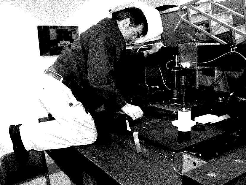
Figure 1: The StarScan plate measuring machine at USNO, Washington DC, with Lars Winter on top of things and Gary Wieder in the background.

Figure 1 shows the StarScan machine as of July 2006. The granite base measures 2.4 by 1.5 by 0.3 meter, and plates up to 260 mm square can be measured. An $x,y$-table moves on the base via pressure air bearings while a CCD camera is mounted on a granite cross-beam which is fixed to the base.

A photographic plate is put inside a plate holder on a rotation disk which is mounted on the $x,y$-table. With emulsion up, the plate is clamped upwards against a fixed mechanical reference plane. Thus the location of the plate emulsion is always at the same distance from the lens and no change in focus is required during operations even if different types of plates are being measured. For very thin plates a supporting clear class plate can be inserted underneath the plate to be measured. The $x,y$-table is moved by precision screws and stepper motors while the coordinates are read from Zerodur Heidenhain scales to better than 0.1 $\mu$m precision.

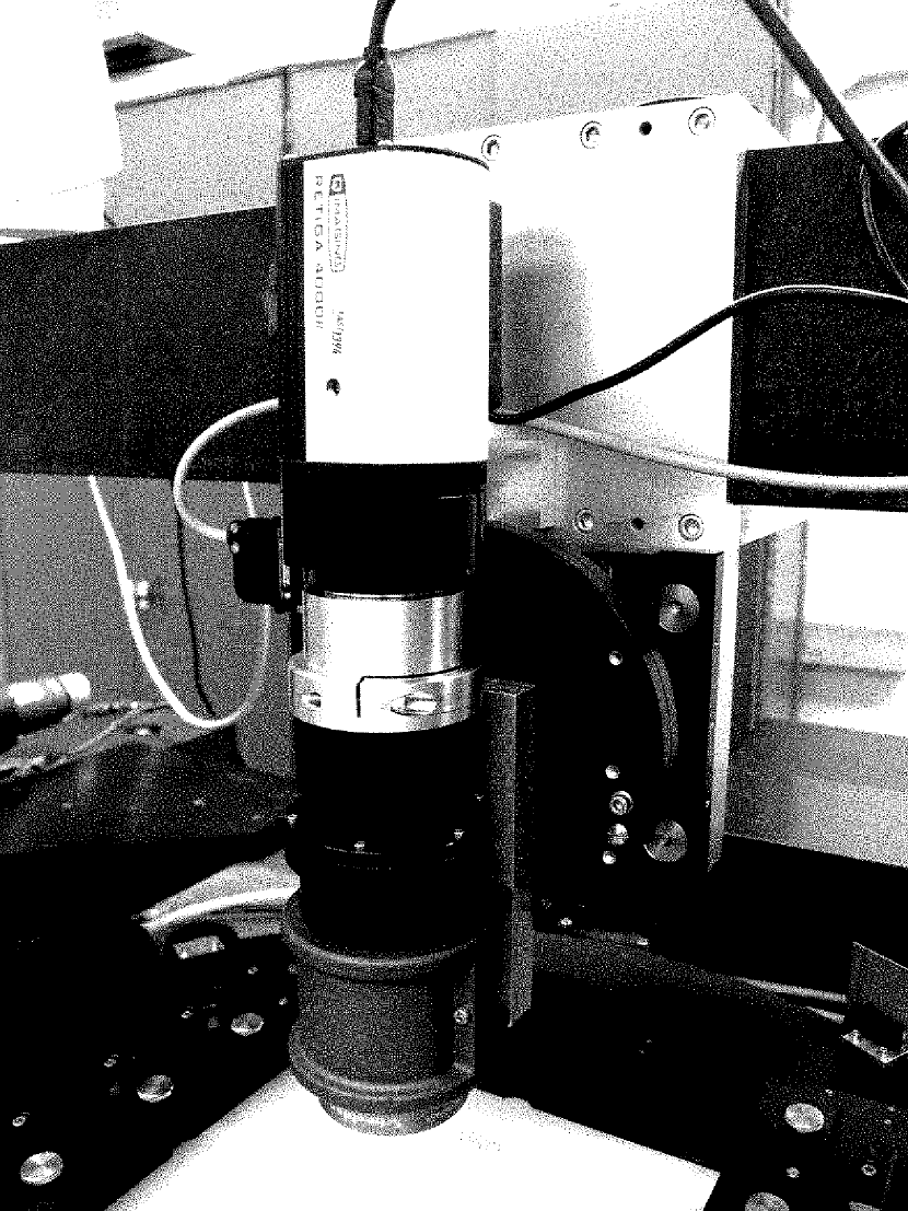
Figure 2: Close-up view of the StarScan plate measure area with the 2k by 2k QImaging camera and Schneider telecentric lens.

The plate is illuminated from below with a diffuse light projection system and a 2-sided telecentric objective (Schneider Xenopla, imaging scale 1:1) maps a section of the plate being measured onto a CCD. From the year 2000 until spring 2006 a Pulnix CCD camera with 1280 by 1030 pixels of 6.7 $\mu$m size was used. Thereafter a 2k by 2k QImaging camera with 7.4 $\mu$m square pixels (Kodak chip) is used. Figure 2 shows a close-up view of the area with the plate and the new CCD camera attached to the lens.

The new camera was selected to be compatible with the existing system in order to minimize changes. However, the upgrade to the new camera did not go smoothly due to various interface issues and in the end a change of the operating system and a complete re-write of large portions of the code was required as well as a new mechanical adapter.

3.2 Measure Process

Most functions, including disk rotation and its clamping mechanism are under computer control. At the beginning of each plate measure the illumination is manually set to just below saturation on the plate background by adjusting the power supply unit to the lamp. Then the plate is measured automatically in step-stare mode. The $x,y$-table moves to the next grid coordinates, the actual table coordinates are obtained by reading out the calibrated Heidenhain scales, a digital image is taken, and another read out of the actual table coordinates is performed. If the table coordinates from the 2 readings differ by more than 0.1 $\mu$m the procedure is repeated. Meanwhile the image is processed: bias, flat field, and dark current corrections, object detection and image profile fits. The entire cycle took about 2.5 sec with the old camera and takes about 4.0 sec with the new camera, which covers about 3 times more area, resulting in an overall throughput gain of a factor of 2.

A photographic plate is thus digitized to 10 bit with a resolution of now $7.4\mu$m per pixel. Adjacent pictures have overlap. The usable field-of-view of the old camera was 8.71 by 6.86 mm, while grid steps of about 7.5 and 5.9 mm for $x$ and $y$, respectively, were used. The new camera has a usable field of about 13 by 13 mm, with slightly degraded image quality (field curvature) visible in the corners. A grid step size of about 11 mm is adopted between adjacent images.

After the plate measure is complete, the disk is unclamped, rotated by $180^{\circ}$, clamped, and the “reverse” measure started. With the new set-up a measure of a single plate in 2 orientations takes about 45 minutes. All pixel data (about 3.6 GB compressed per plate) are transferred overnight and saved to DVD the following day. The stellar image profile fit results are collected on hard disk for further processing.

3.3 Notes on Reductions

The bias, flat field and dark current corrected pixel data of the CCD camera are used in 2-dimensional fits to obtain centroid coordinates of stellar images. A double exponential model function is used for this purpose (Winter, 1999),

$$I(x,y)=B\ +\ A\ (1-e^{-ln2\ e^{-\frac{8}{ln2}\ S\ (r-r_{0})}})$$

$$r=\sqrt{(x-x_{0})^{2}+(y-y_{0})^{2}}$$

with the 6 independent parameters $B$ = background intensity level, $A$ = amplitude, $x_{0},y_{0}$ = image centroid coordinates, $r_{0}$ = radius of profile, and $S$ = shape parameter. This function models the shape of the observed profiles sufficiently well for all levels of brightness of the stars, while e.g. a simple Gaussian function does not match the saturated bright star profiles with “flat tops” very well. Due to the fine sampling (at least 4 pixels across the diameter of the smallest stellar images) a sufficiently large number of pixels contain signal to determine these 6 profile parameters per stellar image. The internal fit precision for all well exposed stars is typically in the order of 0.1 $\mu$m or even below for relatively bright, circular symmetric stellar profiles. For quality control, the internal image profile fit errors are plotted versus the instrumental magnitude for all stellar images of a single plate measure and orientation.

In order to arrive at highly accurate, global $x,y$ coordinates of stellar images from these plate measures several assumptions need to be verified and calibration parameters need to be obtained. Only the center of the CCD chip (or some other, fixed, adopted reference point) is initially associated with the $x,y$-table coordinate readings from the scales. The positions of arbitrary stellar images measured on the CCD chip field-of-view in pixel coordinates need to be referred to the global, $x,y$-table coordinates of the machine, i.e. the mapping model and parameters need to be obtained for this transformation. An important parameter here is the third order optical distortion of the telecentric lens. Using the dot calibration plate (see below) StarScan has been set up to give a mapping scale of 1.0 to within less than a percent and the CCD pixel coordinates are aligned to the global $x,y$-table coordinates to within $10^{-4}$ radian. Also geometric distortions of the observed, global, $x,y$-table coordinates with respect to ideal rectangular coordinates need to be investigated. For both steps, calibrations of the StarScan machine are being made (see below).

Finally, the “direct” and the “reverse” measures of the same plate are compared to check for possible systematic errors e.g. as a function of magnitude or $x,y$ coordinates introduced by the measuring process and to verify that the applied mapping procedures were adequate. The direct-minus-reverse residuals also identified several unexplained glitches of some plate measures, which could have been caused by thermal drifts or electronic problems. The set of the “reverse” measures $X,Y$ (after rotation by $180^{\circ}$) is fit to the “direct” measures ($x,y$) with the following transformation model,

$$X\ =\ a\ x\ +\ b\ y\ +\ c\ +\ e\ x\ +\ f\ y\ +p\ x^{2}\ +\ q\ xy$$

$$Y\ =\ -b\ x\ +\ a\ y\ +\ d\ +\ e\ y\ -\ f\ x\ +q\ y^{2}\ +\ p\ xy$$

where $a,b,c,d$ are the parameters for the orthogonal model, $e,f$ the non-orthogonal, linear parameters, and $p,q$ account for a possible tilt between the 2 sets of measures. On the precision level investigated here the rotation axis of the disk is not perfectly perpendicular to the plane of the plate and the $p,q$ terms are required. These tilt terms are reproducible to some extent, however, sometimes a grain of dust would be trapped between the plate and reference plane of the machine, resulting in significantly different tilt terms. It is important to realize that even after applying the above transformation (and averaging of the $x,y$ coordinates from the “direct” and the ‘rotated “reverse” measures) the data set is affected by an unknown tilt, the tilt of the “direct” measure photographic plate surface with respect to the plane of the $x,y$-table motion. Thus for the astrometric reductions to follow (from $x,y$ to $\alpha,\delta$) the minimal plate model has to include tilt terms as well, even if the tangential point would be known precisely and in the absence of a tilt between the optical axis of the telescope and the photographic plate.

4 Calibration

4.1 Dot calibration plate

The Royal Observatory of Belgium bought a dot calibration plate (DCP) which was made to specifications for the purpose of calibrating photographic plate measuring machines. This 251 mm by 251 mm by 4.6 mm glass plate is highly transparent except for circular, opaque, metal dots of $\approx$ 50 to 300 $\mu$m diameter which are put on the plate in a regular grid covering the inner 240 mm by 240 mm. Medium size dots (100 $\mu$m) occupy a regular grid of 1.0 mm spacing with small dots (50 $\mu$m) put in between every 0.5 mm along both coordinates. In hierarchical order the dots are slightly larger for 5 mm, 10 mm, 50 mm, and 100 mm major grid lines and located at the line intersections of such. The orientation of the grating is uniquely marked by a few out-of-symmetry dots and a missing small dot every cm.

The dot calibration plate was manufactured by silicon wafer technology machines and the location of the dots are believed to be accurate to within about 0.1 to 0.2 $\mu$m for both the small-scale regularity and the global, absolute coordinates over the entire area of the plate.

The dots resemble very high-contrast, stellar images and are processed with the standard reduction pipeline at StarScan. The internal position fit errors of these dots are typically 0.1 $\mu$m for the medium dots on the 1 mm grid, slightly larger for the small 0.5 mm grid dots and even smaller for the major grid dots.

4.2 CCD camera mapping

Initial StarScan mapping parameters for the CCD pixel coordinates to global $x,y$-table coordinates transformation are determined from repeated measures of the dot calibration plate, centered on main grid lines and dithered by small offsets in $x$ and $y$. This in particular allows the determination of the 3rd order optical distortion term $D$ of the lens, which is then used in the preliminary pipeline, together with orientation and scale information, to identify the same star as seen in 2 or more adjacent, overlapping CCD images. Figure 3 shows the residuals of the 2k camera optical distortion pattern after removal of that 3rd order term. The working area used for plate measuring is about 11 by 11 mm. The scale of the residual vectors is 1000, thus the largest residual is about 1.0 $\mu$m, with most of the residuals in the 0.1 to 0.2 $\mu$m range. The point spread function (PSF) of images in the CCD working area is uniform, and there is no variation of the PSF over the area of the plate because there is no variation of best focus over the plate area due to the hardware setup described above.

It is assumed that the mapping parameters stay constant for each individual plate measured in a single orientation, thus all overlap images of such a dataset are used simultaneously to determine the following 7 mapping parameters $a,b,e,f,p,q,D$ from

$$\Delta X\ =\ a\ x\ +\ b\ y\ +\ e\ x\ +\ f\ y\ +p\ x^{2}\ +\ q\ xy\ +\ D\ x(x^{2}+y^{2})$$

$$\Delta Y\ =\ -b\ x\ +\ a\ y\ +\ e\ y\ -\ f\ x\ +q\ y^{2}\ +\ p\ xy\ +\ D\ y(x^{2}+y^{2})$$

where $\Delta X,\Delta Y$ are the coordinates of a star in the global, $x,y$-table system (in millimeter) with respect to the current position as read by the scales, $x,y$ are the stellar image coordinates on the CCD (in pixel) with respect to the center of the CCD. The difference between 2 such equations per coordinate is observed for each pair of overlapping images on 2 CCD frames of the same star.

There are no constant terms because the zero point of this transformation is arbitrary, thus there are only 4 linear terms $a,b,e,f$. The $p,q$ terms represent the tilt between the plane of the CCD chip inside the camera and the photographic plate. The higher order terms for distortion and tilt are almost constant for a large number of plates of the same type and a mean value can be determined and used as fixed parameter in the CCD mapping procedure, while solving then for the linear parameters for each individual plate and orientation measure set with significantly lower errors. Results will be presented in an upcoming paper of this series.

4.3 DCP measures

The DCP was measured in 4 orientations (000, 090, 180, 270 degrees) consecutively with a $x,y$-table step size of 5 mm, major dot grid lines well centered, and grid lines precisely aligned to the table motion. The entire set of measures was repeated about 2 weeks later, with many regular survey plates measured in between. For the present purpose only the central dot of each CCD image has been evaluated which fell on the same spot on the CCD chip within about $\pm$ 10 pixels. Thus any errors introduced by the CCD mapping model are negligible and we measure here the accuracy of the $x,y$-table coordinates of StarScan. In the following we refer to these sets of measures as m1c and m2c, each consisting of 4 single orientation measures of 2025 dots each (on a 220 mm square area with 5 mm step size).

4.4 Repeatability

Without any assumptions on the errors of the DCP a comparison between 2 measures of the same dots in the same measure orientation reveals the absolute repeatability of StarScan measures. Using a linear transformation model between the 2 sets of measures of the 2025 dots gives the results in line 1 through 4 in Table 2 for the root-mean-square (RMS) observed differences per coordinate. The mean of the 4 orientations is presented on line 5 and example 2-dim vector plots of the measured position differences are shown in Figure 4. All vectors are small ($\approx$ 0.3 $\mu$m) but not randomly oriented. For parts of some lines along $x$ they are highly correlated, mainly affecting the $\Delta x$ coordinate. Examples are seen in Figure 4 on the left hand side (for the $90^{\circ}$ orientation case) for $y$ = $-$110, $-$100, $-$30, +40, and +60 mm, and for the $180^{\circ}$ case (right hand side of Figure 4) for $y$ = $-$70, +30, and +50 mm. These glitches are currently not well understood, and seem to appear randomly for a typically length of 50 to 150 mm along the $x$ axis. Some of these errors will cancel out when combining the “direct” and “reverse” measure of a plate. These “glitches” were not further investigated and currently represent the physical limit of the StarScan measure accuracy.

To arrive at the repeatability error ($\sigma_{rep}$) of a single StarScan measure over the entire plate area and per coordinate we divide the RMS differences (Table 2, result line 5, showing the scatter between 2 measures) by $\sqrt{(}2)$ and thus obtain 0.23 and 0.15 $\mu$m for the $x$ and $y$ coordinate, respectively. This error is not dominated by the fit precision of the dots as explained above, instead shows the limit of accuracy of the $x,y$-table coordinate measures.

4.5 Corrections to $x,y$-table coordinates

Next we investigate systematic errors of the $x,y$-table coordinates, i.e. the global, geometric distortions. For each data set (2 measures, each with 4 orientations) a least-squares fit is performed of the measured coordinates to the nominal, ideal grid coordinates, using the above mentioned 8-parameter model which includes linear and tilt terms. Results are presented in Table 2, lines 6 to 13 and for some cases plots are shown in Figure 5. As can be seen the difference vectors are highly correlated among the different plots, indicating that the dominating error source is systematics in the StarScan $x,y$-table geometry, due to imperfections of the axes as the plate is moved along in the measuring process. If the DCP would have large errors as compared to StarScan, the rotated measures ($90^{\circ}$ and $180^{\circ}$) would show the same pattern as the “direct” measure (orientation $0^{\circ}$) but rotated by that angle. However, we see here the systematic error pattern correlated directly to the StarScan $x,y$ coordinates, regardless of the orientation of the calibration plate.

A mean 2-dimensional vector difference map was constructed by averaging all 8 measures (2 sets times 4 orientations each) and then applying a near neighbor smoothing. Results are given on line 14 in Table 2 and the corresponding vector plot is shown in Figure 6. Subtracting this mean pattern from the individual measure sets (Table 2, lines 6 to 13) results in lines 15 to 22 with RMS values almost as low as the StarScan repeatability, showing the successful removal of most of the $x,y$-table systematic errors.

5 Application to Real Data

5.1 Different plates of the same field

In order to determine the physical limit of astrograph plates for astrometry a set of 4 different plates taken of the same field (2234+282) in the sky is investigated. The 4 plates were taken in 1988 with the Hamburg Zone Astrograph (ZA) (de Vegt, 1976) in the same night within 40 minutes off the meridian through an OG515 filter on 103aG emulsion. Plate numbers 1929 and 1930 were taken with the telescope on the West side of the pier, numbers 1931 and 1932 on East. Here we assume that the StarScan measure errors are small and we will try to determine total external errors from the combination of plate geometry (emulsion shifts) over the entire field of view and the background noise from the emulsion grains, using real stellar images.

A transformation of the “direct” measure of ZA1930 onto the “direct” measure of ZA1929 was performed using the above mentioned 8-parameter model and using about 19,000 stellar images in an unweighted, least-squares fit. A 5-parameter mapping model including linear and tilt terms was used for the CCD camera mapping, after applying a mean optical distortion term to the raw data. No $x,y$-table corrections of StarScan were applied because they would cancel anyway in this “direct” to “direct” transformation (assuming stability of the machine over a few hours in which the set of plates were measured). Table 2, lines 23 to 26 show the mean RMS differences for “well exposed” stars (about 10th magnitude) between the 2 plates. Thus the external error of a single, well exposed stellar image on a single plate is about 0.65 $\mu$m per coordinate.

This number reflects the sum of the StarScan measure errors and the errors inherent in the photographic material, and is dominated by the grain noise of this type of emulsion, consistent with previous investigations (Auer & van Altena, 1978). However, these numbers do not directly translate into $\alpha,\delta$ accuracies. In order to get highly accurate astrometric positions on the sky from these calibrated, measured $x,y$ data the systematic errors introduced by the astrograph (optics, guiding etc.) and the atmosphere need to be detected, quantified and removed.

5.2 Long term repeatability and discussion

A fine grain (Kodak Technical Pan emulsion) plate (No. 724) of a dense field (NGC 6791) obtained at the Lick 50cm astrograph has been measured multiple times during the StarScan operations at relatively regular intervals to monitor its performance. Contrary to the DCP, the location of the “dots” on this plate are not known apriori; however, they are “fixed” and StarScan should measure the same positions of these stellar images (within its errors) every time it has been measured. Thus these data sets provide information about the long-term stability and repeatability of the StarScan measures and shed some light on the validity of using “the” $x,y$-table correction pattern as derived in the previous section.

Results are given in Table 2 for measures 1,6,9, and “a” (lines 27 to 30), which correspond to May 2004, Sept 2004, Sep 2005, and Apr 2006, respectively. For each data set the plate was measured in ”direct” (000) and “reverse” (180) orientation and the 8-parameter model was used in a least-squares adjustment in the transformation between the orientations $x,y$ data after applying the same 2-dim table corrections as presented above to all measures.

Figure 7 shows the residuals of such a transformation for the measure # 6 (September 2004) of that Lick plate. As an example the $x$ residuals are shown as a function of $x$, $y$, and magnitude. There is a magnitude equation of about 0.3 $\mu$m amplitude for $x$, while there is none for the $y$ coordinate (not shown here). Residuals as a function of the coordinates still show systematic errors up to about 0.5 $\mu$m, even after applying the 2-dim $x,y$ table corrections. The high frequency wiggles are likely caused by the residual CCD camera mapping errors, while the low frequency systematic errors are likely deviations of the $x,y$ table corrections as applied with respect to what actually is inherent in the data at the time of the measurement.

In order to better illustrate the long-term variability, Figure 8 shows only the $x$ residual versus $y$ plot but for 3 other measures of the same plate (May 2004, September 2005, and April 2006), which should be compared to the middle diagram of Figure 7. Clearly there are variations over time, however the overall correction is good to about 0.4 $\mu$m per coordinate, with the RMS error being much smaller.

Part of the remaining systematic pattern is clearly correlated with the location of stellar images on the CCD area. This is caused by an imperfect model in mapping from the CCD pixel coordinates to the $x,y$ table coordinate system. This is not surprising considering that the poorest image quality of the CCD area (ther corner and border areas) are utilized to determine those mapping parameters, and an extrapolation to the entire CCD area has to be made. Measuring plates with significantly larger overlap between adjacent CCD images would help to even lower those type of errors. However, as other error sources indicate, we have reached the overall StarScan accuracy limit and allowing a significantly larger overlap would have increased the project time significantly with little benefit. The HAM-I measuring machine Zacharias et al. (1994) completely eliminated this problem by centering each star to be measured on the CCD image. However, that required an a priori measure list and a very long measure time, but an astrometric accuracy similar to that of StarScan was obtained.

It is not possible to correct the measures for the remaining systematic errors as a function of the coordinates based on findings like Figures 7 and 8 because the differences between the “direct” and “reverse” measure are seen here, while the combined, mean measured position of each star would be based on the sum of the measures. Comparisons like these for the residuals as a function of the coordinates serve as check of the data and applied models, and are indicative for such systematic errors staying constant which allows to group plate measures correctly in further reduction steps.

The situation is much different for the magnitude dependent systematic errors. Assuming that the magnitude equation is constant for both orientation measures, it automatically drops out when combining the “direct” and “reverse” measures, while twice the deviation of a single measure with respect to the error free data is seen in the residual plot as a function of magnitude. If only a single plate orientation were measured this magnitude equation would need to be determined and corrected by some other means, which would be hard to do.

6 Summary and Conclusions

For well exposed stellar images StarScan has a repeatability error of 0.2$\mu$m per coordinate. Using overlapping areas in the digitization process the mapping parameters of the CCD camera with respect to the $x,y$-table coordinate system are calibrated for each plate and orientation measure to the same precision. The overall accuracy of StarScan measures is limited by the systematic errors of the $x,y$-table and the stage motions. Using a dot calibration plate specifically manufactured for this purpose, 2-dimensional correction data are obtained to calibrate the $x,y$-table coordinate system. The high precision of the StarScan measures allows one to see variations in this calibration pattern which depend at least on time, maybe on other parameters as well. The uncalibrated machine performs at an accuracy level of about 1 $\mu$m RMS with a parabola-like distortion for the $\Delta y$ as a function of $y$ with $\pm$ 1.5 $\mu$m amplitude being the largest error contribution. After applying the 2-dim calibration corrections StarScan performs on the 0.3 $\mu$m per coordinate accuracy level.

By comparing different photographic plates of the same field it has been demonstrated that astrometric useful information at an accuracy level of at least 0.65 $\mu$m can be extracted from the data of course grain emulsions exposed at dedicated astrographs. Comparisons of “direct” and “reverse” measures of fine grain emulsions show errors of 0.3 $\mu$m per single star image and measure. This is only an upper limit of the plate data quality, because of StarScan measuring machine errors close to the same level. A higher accuracy than StarScan currently can provide is recommended for fine grain astrometric plates and such a new machine was just delivered to the Royal Observatory Belgium (De Cuyper & Winter, 2006).

It is recommended to measure the dot calibration plate often to verify and improve the 2-dim $xy$-table corrections. Measuring a plate in 2 orientations, rotated by $180^{\circ}$, is mandatory, at least for StarScan and when aiming at high accuracy metric results, in order to correct for the non-linear magnitude equation from the measure process and to monitor quality by identifying occasional problems in the measure process.

Table 1: Astrometric plates in the just completed StarScan measure program. The AGK2 covers each area of the northern sky twice (2-fold overlap of plates). The BY (south) and ZA (north) programs together cover about 35% of the entire sky area.

project, telescope name	AGK2	BY	ZA	Lick
focal length (meter)	2.0	2.0	2.0	3.75
plate size (mm)	220 sq.	200 x 250	240 sq.	240 sq.
measurable field size (degree)	5 x 5	5 x 6	6 x 6	3 x 3
limiting magnitude	B = 12	V = 14	V = 14	V = 15
number of plates	1940	900	2200	300
range of epochs	1929–31	1985–90	1977–93	1980–2000
emulsion type	fine grain	103aG	103aG	various
declination range (degree)	$-$2.5 +90	$-$90 +10	$-$5 +90	$-$20 +90
sky coverage completeness	2-fold	35%	35%	5%

Table 2: Results of transformations between 2 sets of data, DCP = dot calibration plate, m1c, m2c = sets 1 and 2 of measures of central dots, and 000 to 270 indicate the orientation of a measure. See text for more details.

result	data set 1	data set 2	model	RMS x	RMS y
number				($\mu$m)	($\mu$m)
1	DCP m1c 000	DCP m2c 000	linear	0.31	0.20
2	DCP m1c 090	DCP m2c 090	linear	0.34	0.24
3	DCP m1c 180	DCP m2c 180	linear	0.30	0.15
4	DCP m1c 270	DCP m2c 270	linear	0.33	0.23
5	mean of 1–4			0.32	0.21
6	DCP m1c 000	ideal grid	lin.+ tilt	0.41	0.44
7	DCP m1c 090	ideal grid	lin.+ tilt	0.47	0.53
8	DCP m1c 180	ideal grid	lin.+ tilt	0.36	0.56
9	DCP m1c 270	ideal grid	lin.+ tilt	0.40	0.42
10	DCP m2c 000	ideal grid	lin.+ tilt	0.40	0.40
11	DCP m2c 090	ideal grid	lin.+ tilt	0.44	0.57
12	DCP m2c 180	ideal grid	lin.+ tilt	0.37	0.53
13	DCP m2c 270	ideal grid	lin.+ tilt	0.48	0.40
14	mean, smoothed 2-dim $x,y$-table corrections			0.27	0.39
15	result 6	mean corrections	none	0.32	0.33
16	result 7	mean corrections	none	0.35	0.23
17	result 8	mean corrections	none	0.28	0.32
18	result 9	mean corrections	none	0.31	0.20
19	result 10	mean corrections	none	0.28	0.32
20	result 11	mean corrections	none	0.30	0.26
21	result 12	mean corrections	none	0.28	0.27
22	result 13	mean corrections	none	0.37	0.27
23	ZA 1929 000	ZA 1930 000	lin.+ tilt	0.89	0.85
24	ZA 1929 180	ZA 1930 180	lin.+ tilt	0.84	0.89
25	ZA 1931 000	ZA 1932 000	lin.+ tilt	0.92	0.92
26	ZA 1931 180	ZA 1932 180	lin.+ tilt	0.92	0.92
27	Lick 724 m1 000	Lick 724 m1 180	lin.+ tilt	0.41	0.68
28	Lick 724 m6 000	Lick 724 m6 180	lin.+ tilt	0.40	0.35
29	Lick 724 m9 000	Lick 724 m9 180	lin.+ tilt	0.42	0.49
30	Lick 724 ma 000	Lick 724 ma 180	lin.+ tilt	0.45	0.45

Figure 3: Optical distortion pattern of the 2k camera field of view after removal of the 3rd order term. The residual vectors are scaled by a factor of 1000, thus the largest vector is about 1.0 $\mu$m long. Results are shown in the about 11 by 11 mm area of the detector which is used for plate measuring.

Figure 4: Repeatability: vector plot of position differences between 2 measures of the same dot calibration plate in the same orientation, performed on different days. The examples show the worst (left) and best (right) case ($90^{\circ}$ and $180^{\circ}$ orientation, respectively). The scale is 5000 thus the largest vectors are about 1.0 $\mu$m long, and the RMS vector length is 0.42 and 0.33 $\mu$m, respectively.

Figure 5: Differences between individual orientation measures of the dot calibration plate (DCP) and the ideal grid coordinates after a least-squares fit with an 8-parameter transformation model. The scale is 5000 thus the largest vectors are about 1.5 $\mu$m long. The top plots show results for the same orientation ($0^{\circ}$) from the first and second set. The plots at the bottom show more results from the first set for the $90^{\circ}$ and $180^{\circ}$ orientation measures.

Figure 6: Mean StarScan $x,y$-table corrections. This pattern was derived by taking the smoothed average over all 8 vector plots of which some are shown in Figure 4. The scale is 5000 thus the largest vectors are about 1.0 $\mu$m long.

Figure 7: Data of Lick Astrograph plate 724 measured in 2 orientations in September 2004 (measure # 6). The “direct” minus “reverse” residuals in $x$ are shown as a function of $x$, $y$, and magnitude (top to bottom). Each dot is the average over 25 stars, thus highlighting the systematic errors.

Figure 8: Data of Lick Astrograph plate 724 measured in 2 orientations. The “direct” minus “reverse” residuals in $x$ are shown as a function of $y$ for 3 different measure dates (from top to bottom): May 2004 (m.1), September 2005 (m.9), and April 2006 (m.a) Each dot is the average over 25 stars, thus highlighting the systematic errors.

References

- Auer & van Altena (1978) Auer, L. H., van Altena, W. 1978, AJ 83, 531
- de Vegt (1976) de Vegt, C. 1976, Mit. AG, 38, 181
- de Vegt (1978) de Vegt, C. 1978, in “Modern Astrometry”, in proceed. IAU Col. 48, Eds. F. V. Prochazka & R. H. Tucker, p. 527
- De Cuyper & Winter (2006) De Cuyper, J.-P., Winter,L. 2006, in proceed. ADAS XV, ASP Conference Series, Vol. 351, p587-590, C. Gabriel, C. Arviset, D. Ponz and E. Solano, eds.
- ESA (1997) ESA, 1997, The Hipparcos Catalogue, ESA SP-1200
- Douglass et al. (1990) Douglass, G.G. & Harrington, R. S. 1990, AJ 100, 1712
- Høg et al. (2000) Høg et al. 2000, A&A, 355, L27
- Schorr & Kohlschütter (1951) Schorr, R., Kohlschütter, A. 1951, Zweiter Katalog der Astronomischen Gesellschaft, AGK2, Volume I (Hamburg: Bonn and Hamburg Observatories)
- Winter (1999) Winter, L. 1999, PhD thesis, Univ. of Hamburg
- Winter & Holdenried (2001) Winter, L. & Holdenried, E. 2001, BAAS, 33 - 4, sect. 129,3
- Zacharias et al. (1994) Zacharias, N., de Vegt, C., Winter, L. & Weneit, W., in Proceed. IAU Sympos. 161, p. 285, Eds. H. T. MiacGillivray et al., Kluwer Acad. Publ. 1994
- Zacharias & Zacharias (1999) Zacharias, N. & Zacharias, M.I. 1999, AJ, 118, 2503
- Zacharias et al. (2000) Zacharias, M. I., Hall, D. G., Wycoff, G. L., Rafferty, T. J., Germain, M. E., Holdenried, E. R., Pohlman, J. W., Gauss, F. S., Monet, D. G., & Winter, L. 2000, AJ, 120, 2131
- Zacharias et al. (2004) Zacharias, N., Urban, S.E., Zacharias, M.I., Wycoff, G.L., Hall, D.M., Monet, D.G., Rafferty, T.J. 2004, AJ 127, 3043