The Dirichlet problem for the minimal surface equation -with possible infinite boundary data- over domains in a Riemannian surface

1 Introduction

In [8], Jenkins and Serrin considered bounded domains $D\subset{\mathbb{R}}^{2}$, with $\partial D$ composed of straight line segments and convex arcs. They found necessary and sufficient conditions on the lengths of the sides of inscribed polygons, which guarantee the existence of a minimal graph over $D$, taking certain prescribed values (in ${\mathbb{R}}\cup\{\pm\infty\}$) on the components of $\partial D$

Perhaps the simplest example is $D$ a triangle and the boundary data is zero on two sides and $+\infty$ on the third side. The conditions of Jenkins-Serrin reduce to the triangle inequality here and the solutions exists. It was discovered by Scherk in 1835.

This also works on a parallelogram with sides of equal length. One prescribes $+\infty$ on opposite sides and $-\infty$ on the other two sides. This solution was also found by Scherk.

The theorem of Jenkins and Serrin also applies to some non-convex domains. They only require $\partial D$ to be composed of a finite number of convex arcs, together with their endpoints.

In a very interesting paper [17], Joel Spruck solved the Dirichlet problem for the constant mean curvature $H$ equation over bounded domains $D\subset{\mathbb{R}}^{2}$, with $\partial D$ composed of circle arcs of curvature $\pm 2H$, together with convex arcs of curvature larger than $2H$. The boundary data now is $\pm\infty$ on the circle arcs and prescribed continuous data on the convex arcs. He gave necessary and sufficient conditions on the perimeter, and area, of inscribed polygons that solve the Dirichlet problem.

In recent years there has been much activity on this Dirichlet problem over domains $D$ contained in a Riemannian surface ${\mathbb{M}}$ [14, 18]. When ${\mathbb{M}}$ is the hyperbolic plane ${\mathbb{H}}^{2}$, there are non-compact domains for which this problem has been solved, and interesting applications have been obtained (see for example [3, 6, 11]

In this paper we will extend the solution of this Dirichlet problem to general domains. In the case of a Riemannian surface ${\mathbb{M}}$, we consider non-convex domains (see Section 3). For ${\mathbb{M}}={\mathbb{H}}^{2}$, we study non-compact domains.

Our techniques for doing this in ${\mathbb{H}}^{2}$ are new (and apply to domains in arbitrary ${\mathbb{M}}$). Previously one found a solution to the Dirichlet problem by taking limits of monotone sequences of solutions whose boundary data converges to the prescribed data. A basic tool to make this work is the maximum principle for solutions: if $u$ and $v$ are solutions and $u\leq v$ on $\partial D$, then $u\leq v$ on $D$. However, there are domains for which the maximum principle fails (we discuss this in Section 4.3.2). In order to solve the Dirichlet problem in the absence of a maximum principle we use the idea of divergence lines introduced by Laurent Mazet in his thesis [9]. This enables us to obtain convergent subsequences of non-necessarily monotone sequences.

This lack of a general maximum principle implies that one no longer has uniqueness (up to an additive constant, in the case of infinite boundary data) for the solutions. In section 4.3, we obtain uniqueness theorems for certain domains and we give examples where this fails.

2 Preliminaries

From now on, ${\mathbb{M}}$ will denote a Riemannian surface. In the following, div, $\nabla$ and $|\cdot|$ are defined with respect to the metric on ${\mathbb{M}}$. Let $\Omega$ be a domain in ${\mathbb{M}}$ and $u:\Omega\to{\mathbb{R}}$ be a smooth function. We define $W_{u}=\sqrt{1+|\nabla u|^{2}}$. The graph of such a smooth function $u$ that satisfies

$$\mbox{div}\left(\frac{\nabla u}{W_{u}}\right)=0,$$

is a minimal surface in ${\mathbb{M}}\times{\mathbb{R}}$; referred to as a minimal graph. In the following we will denote $X_{u}=\frac{\nabla u}{W_{u}}$.

The next results have been proven by Jenkins and Serrin [8] for ${\mathbb{M}}={\mathbb{R}}^{2}$, by Nelli and Rosenberg [11] when ${\mathbb{M}}={\mathbb{H}}^{2}$, and by Pinheiro [14] in the general setting. In fact, these results were proven for bounded and geodesically convex domains in [14], although their proofs remain valid in a more general setting.

Theorem 2.1 (Compactness theorem).

Let $\{u_{n}\}$ be a uniformly bounded sequence of minimal graphs in a bounded domain $\Omega\subset{\mathbb{M}}$. Then, there exists a subsequence of $\{u_{n}\}$ converging on compact subsets of $\Omega$ to a minimal graph $u$ on $\Omega$.

Theorem 2.2 (Monotone convergence theorem).

Let $\{u_{n}\}$ be an increasing sequence of minimal graphs on a domain $\Omega\subset{\mathbb{M}}$. There exists an open set ${\cal U}\subset\Omega$ (called the convergence set) such that $\{u_{n}\}$ converges uniformly on compact subsets of ${\cal U}$ and diverges uniformly to $+\infty$ on compact subsets of ${\cal V}=\Omega-\overline{\cal U}$ (divergence set). Moreover, if $\{u_{n}\}$ is bounded at a point $p\in\Omega$, then the convergence set ${\cal U}$ is non-empty (it contains a neighborhood of $p$).

Now we recall some results which allow us to describe the divergence set ${\cal V}$ associated to a monotone sequence of minimal graphs.

Lemma 2.3 (Straight line lemma).

Let $\Omega\subset{\mathbb{M}}$ be a domain, $C\subset\partial\Omega$ a convex compact arc, and $u\in{\cal C}^{0}(\Omega\cup C)$ a minimal graph on $\Omega$. Denote by ${\cal C}(C)$ the (open) convex hull of $C$.

• If $u$ is bounded above on $C$ and $C$ is strictly convex, then $u$ is bounded above on $K\cap\Omega$, for every compact set $K\subset{\cal C}(C)$.

• If $u$ diverges to $+\infty$ or $-\infty$ as we approach $C$ within $\Omega$, then $C$ is a geodesic arc.

Definition 2.4.

Let $u$ be a minimal graph on a domain $\Omega\subset{\mathbb{M}}$ and assume that $\partial\Omega$ is arcwise smooth. When $C$ is an arc in $\Omega$ and $\nu$ is a unit normal to $C$ in ${\mathbb{M}}$ we define the flux of $u$ across $C$ for such choice of $\nu$ by

$$F_{u}(C)=\int_{C}\langle X_{u},\nu\rangle ds,$$

where $ds$ is the arc length of $C$. Since the vector field $X_{u}$ is bounded and has vanishing divergence, the flux is also defined across a curve $\Gamma\subset\partial\Omega$, in that case, $\nu$ is chosen to be the outer normal to $\partial\Omega$.

In the paper, when a flux is computed across a curve $C$, the curve $C$ will be always seen as part of the boundary of a subdomain. The normal $\nu$ will then be chosen as the outer normal to the subdomain.

Lemma 2.5.

Let $u$ be a minimal graph on a domain $\Omega\subset{\mathbb{M}}$.

• For every compact bounded domain $\Omega^{\prime}\subset\Omega$, we have $F_{u}(\partial\Omega^{\prime})=0$.

• Let $C$ be a piecewise smooth interior curve or a convex curve in $\partial\Omega$ where $u$ extends continuously and takes finite values. Then $|F_{u}(C)|<|C|$.

• Let $T\subset\partial\Omega$ be a geodesic arc such that $u$ diverges to $+\infty$ (resp $-\infty$) as one approaches $T$ within $\Omega$. Then $F_{u}(T)=|T|$ (resp. $F_{u}(T)=-|T|$).

Remark 2.6.

From Lemma 2.5 and the triangle inequality, we deduce that, if $u:\Omega\to{\mathbb{R}}$ is a minimal graph and $T_{1},T_{2}\subset\partial\Omega$ are two geodesics where $u$ diverges to $+\infty$ as we approach them, then $T_{1},T_{2}$ cannot meet at a strictly convex corner (strictly convex with respect to $\Omega$).

The last statement in Lemma 2.5 admits the following generalization.

Lemma 2.7.

For each $n\in{\mathbb{N}}$, let $u_{n}$ be a minimal graph on a fixed domain $\Omega\subset{\mathbb{M}}$ which extends continuously to $\overline{\Omega}$, and let $T$ be a geodesic arc in $\partial\Omega$.

• If $\{u_{n}\}$ diverges uniformly to $+\infty$ on compact sets of $T$ while remaining uniformly bounded on compact sets of $\Omega$, then $F_{u_{n}}(T)\to|T|$.

• If $\{u_{n}\}$ diverges uniformly to $+\infty$ on compact sets of $\Omega$ while remaining uniformly bounded on compact sets of $T$, then $F_{u_{n}}(T)\to-|T|$.

The following result is adapted to the situation of the next section. The boundary of a domain $\Omega$ is finitely piecewise smooth and locally convex if it is composed of a finite number of open smooth arcs which are convex towards $\Omega$, together with their endpoints. These endpoints are called the vertices of $\Omega$.

Theorem 2.8 (Divergence set theorem).

Let $\Omega\subset{\mathbb{M}}$ be a bounded domain with finitely piecewise smooth and locally convex boundary. Let $\{u_{n}\}$ be an increasing (resp. decreasing) sequence of minimal graphs on $\Omega$. For every open smooth arc $C\subset\partial\Omega$, we assume that, for every $n$, $u_{n}$ extend continuously on $C$ and either $u_{n}|_{C}$ converges to a continuous function or $u_{n}|_{C}\nearrow+\infty$ (resp. $u_{n}|C\searrow-\infty$). Let ${\cal V}$ be the divergence set associated to $\{u_{n}\}$

1. The boundary of ${\cal V}$ consists of a finite set of non-intersecting interior geodesic chords in $\Omega$ joining two vertices of $\partial\Omega$, together with geodesics in $\Omega$.

2. A component of ${\cal V}$ cannot only consist of an isolated point nor an interior chord.

3. No two interior chords in $\partial{\cal V}$ can have a common endpoint at a convex corner of ${\cal V}$.

Theorem 2.9 (Maximum principle for bounded domains).

Let $\Omega\subset{\mathbb{M}}$ be a bounded domain, and $E\subset\partial\Omega$ a finite set of points. Suppose that $\partial\Omega\backslash E$ consists of smooth arcs $C_{k}$, and let $u_{1},u_{2}$ be minimal graphs on $\Omega$ which extend continuously to each $C_{k}$. If $u_{1}\leq u_{2}$ on $\partial\Omega\backslash E$, then $u_{1}\leq u_{2}$ on $\Omega$.

Theorem 2.10 (Boundary values lemma).

Let $\Omega\subset{\mathbb{M}}$ be a domain and let $C$ be a compact convex arc in $\partial\Omega$. Suppose $\{u_{n}\}$ is a sequence of minimal graphs on $\Omega$ converging uniformly on compact subsets of $\Omega$ to a minimal graph $u:\Omega\to{\mathbb{R}}$. Assume each $u_{n}$ is continuous in $\Omega\cup C$ and $\{u_{n}|_{C}\}$ converges uniformly to a function $f$ on $C$. Then $u$ is continuous in $\Omega\cup C$ and $u|_{C}=f$.

3 A general Jenkins-Serrin theorem on ${\mathbb{M}}\times{\mathbb{R}}$

Let $\Omega\subset{\mathbb{M}}$ be a bounded domain whose boundary consists of a finite number of open geodesic arcs $A_{1},\cdots,A_{k_{1}},B_{1},\cdots,B_{k_{1}}$ and a finite number of open convex arcs $C_{1},\cdots,C_{k_{3}}$ (convex towards $\Omega$), together with their endpoints. We mark the $A_{i}$ edges by $+\infty$, the $B_{i}$ edges by $-\infty$, and assign arbitrary continuous data $f_{i}$ on the arcs $C_{i}$.

Definition 3.1.

We define a solution for the Dirichlet problem on $\Omega$ as a minimal graph $u:\Omega\to{\mathbb{R}}$ which assumes the above prescribed boundary values on $\partial\Omega$.

Our aim in this section is to solve this Dirichlet problem on $\Omega$. We assume that no two $A_{i}$ edges and no two $B_{i}$ edges meet at a convex corner (see Remark 2.6). When $\Omega$ is geodesically convex, this was done in [14]; in general we need another condition on the $\partial\Omega$. We assume the following technical condition is satisfied:

• If $\{C_{i}\}_{i}=\emptyset$, then neither $\cup_{i=1}^{k_{1}}\overline{A_{i}}$ nor $\cup_{i=1}^{k_{2}}\overline{B_{i}}$ is a connected subset of $\partial\Omega$.

We will say that a domain $\Omega$ as above is a Scherk domain. We notice that the hypothesis (C1) implies that $k_{1}\geq 2$ and $k_{2}\geq 2$ when $\{C_{i}\}_{i}=\emptyset$. We remark that (C1) is always satisfied when ${\mathbb{M}}={\mathbb{R}}^{2},{\mathbb{H}}^{2}$.

Condition (C1) is not necessary for the existence of a solution to the Dirichlet problem on $\Omega$ (see Remark 3.5) but we need to assume this for our proof.

Claim 3.2.

In particular, condition (C1) holds when there exists a component $\Gamma$ of $\partial\Omega$ and a strongly geodesically convex domain $\Omega^{\prime}\subset{\mathbb{M}}$ containing $\Omega$ such that $\partial\Omega^{\prime}=\Gamma$.

Suppose $\{C_{i}\}_{i}=\emptyset$. Since $\Gamma$ is the boundary of $\Omega^{\prime}$ and $\overline{\Omega^{\prime}}$ is geodesically convex, we can rename the $A_{i},B_{i}$ edges so that $\Gamma=A_{1}$ or $\Gamma=B_{1}$ or $\Gamma=A_{1}\cup B_{1}\cup\cdots\cup A_{k}\cup B_{k}$ (cyclically ordered). The first two cases are not allowed: in fact, in that cases $A_{1}$ or $B_{1}$ would be closed and two points on it would be joined by two geodesic arcs in $\Gamma\subset\overline{\Omega^{\prime}}$.

In the third case, we have $k\geq 2$. If $k=1$, the common endpoints of $A_{1}$ and $B_{1}$ are joined by two geodesic arcs, $A_{1}$ and $B_{1}$, in $\overline{\Omega^{\prime}}$ which is impossible. Thus $k\geq 2$ and (C1) holds.

A polygonal domain ${\cal P}$ is said to be inscribed in $\Omega$ when ${\cal P}\subset\Omega$ and its vertices are drawn from the set of endpoints of the $A_{i},B_{i},C_{i}$ edges. Given a polygonal domain ${\cal P}$ inscribed in $\Omega$, we denote by $\gamma$ the perimeter of $\partial{\cal P}$, and by $\alpha$ (resp. $\beta$) the total length of the edges $A_{i}$ (resp. $B_{i}$) lying in $\partial{\cal P}$.

Theorem 3.3.

Let $\Omega$ be a Scherk domain. If the family $\{C_{i}\}_{i}$ is non-empty, there exists a solution to the Dirichlet problem on $\Omega$ if and only if

$$2\alpha<\gamma\qquad\mbox{and }\qquad 2\beta<\gamma$$ (1)

for every polygonal domain ${\cal P}$ inscribed in $\Omega$. Moreover, such a solution is unique, if it exists.

When $\{C_{i}\}_{i}$ is empty, there is a solution to the Dirichlet problem for $\Omega$ if and only if $\alpha=\beta$ when ${\cal P}=\Omega$, and inequalities in (1) hold for all other polygonal domains inscribed in $\Omega$. Such a solution is unique up to an additive constant, if it exists.

Remark 3.4.

1. The Scherk domain $\Omega$ need not be convex, even when there are no $A_{i}$ and $B_{j}$ edges. There are no conditions in the latter case; the solution need not be continuous at the vertices.

2. Theorem 3.3 corresponds to Theorem 4 in [8], in the case ${\mathbb{M}}={\mathbb{R}}^{2}$.

3. Theorem 3.3 has been proven, when $\Omega$ is a geodesically convex domain, by Nelli and Rosenberg [11] (in the case ${\mathbb{M}}={\mathbb{H}}^{2}$) and by Pinheiro [14].

The uniqueness part in Theorem 3.3 can be proven exactly as in [14]. Let us now prove the conditions of Theorem 3.3 are necessary for existence. Suppose there is a minimal graph $u$ solving the Dirichlet problem. When $\{C_{i}\}_{i}=\emptyset$ and ${\cal P}=\Omega$, using Lemma 2.5 we have

$$\textstyle{\alpha=\sum_{i}|A_{i}|=\sum_{i}F_{u}(A_{i})=-\sum_{i}F_{u}(B_{i})=\sum_{i}|B_{i}|=\beta,}$$

as we wanted to prove. In the other case, again by Lemma 2.5, we obtain:

• $\sum_{A_{i}\subset\partial{\cal P}}F_{u}(A_{i})+\sum_{B_{i}\subset\partial{\cal P}}F_{u}(B_{i})+F_{u}(\partial{\cal P}-\cup_{i}A_{i}-\cup_{i}B_{i})=0$.

• $\sum_{A_{i}\subset\partial{\cal P}}F_{u}(A_{i})=\sum_{A_{i}\subset\partial{\cal P}}|A_{i}|=\alpha$.

• $\sum_{B_{i}\subset\partial{\cal P}}F_{u}(B_{i})=-\sum_{B_{i}\subset\partial{\cal P}}|B_{i}|=-\beta$.

• $|F_{u}(\partial{\cal P}-\cup_{i}A_{i}-\cup_{i}B_{i})|<\gamma-\alpha-\beta$.

From all this, $|\alpha-\beta|<\gamma-\alpha-\beta$, so $2\alpha<\gamma$ and $2\beta<\gamma$, as desired.

Finally, let us prove the conditions are sufficient. We distinguish the following cases:

$\star$ First case: Suppose that the families $\{A_{i}\}_{i},\{B_{i}\}_{i}$ are both empty.
In this case, Theorem 3.3 is proven, exactly as in [8] for ${\mathbb{M}}={\mathbb{R}}^{2}$, by means of the Perron process (see [5, 8]), using the fact that the solution to the Dirichlet problem exists for small geodesic disks [14] and a standard barrier argument (a barrier exists at every convex boundary point, see [14]).

$\star$ Second case: Suppose $\{B_{i}\}_{i}=\emptyset$ and each $f_{i}$ is bounded below.
Using the previous step, there exists, for every $n\in{\mathbb{N}}$, a unique minimal graph ${u_{n}:\Omega\to{\mathbb{R}}}$ such that:

$$\left\{\begin{array}[]{lllll}u_{n}=n&\mbox{, on the }A_{i}\mbox{ edges.}\\ u_{n}=\min\{n,f_{i}\}&\mbox{, on the }C_{i}\mbox{ edges.}\\ \end{array}\right.$$

From the maximum principle for bounded domains (Theorem 2.9), we deduce that $\{u_{n}\}$ is a non-decreasing sequence. Thus Lemma 2.3 and Theorem 2.8 assure that, if it is non-empty, the divergence set ${\cal V}$ of $\{u_{n}\}$ consists of a finite number of polygonal domains inscribed in $\Omega$. Assume that ${\cal V}$ is connected (otherwise, we will similarly argue on each component of ${\cal V}$). By Lemma 2.5, the flux of $u_{n}$ along $\partial{\cal V}$ vanishes; this is,

$$\sum_{A_{i}\subset\partial{\cal V}}F_{u_{n}}(A_{i})+F_{u_{n}}(\partial{\cal V}-\cup_{i}A_{i})=0.$$

On the other hand, Lemma 2.7 says that $F_{u_{n}}(\partial{\cal V}-\cup_{i}A_{i})\rightarrow-(\gamma-\alpha)$ as $n\rightarrow+\infty$. Since $\sum_{A_{i}\subset\partial{\cal V}}|F_{u_{n}}(A_{i})|\leq\alpha$, we obtain $2\alpha-\gamma\geq 0$, which contradicts (1). Hence ${\cal V}=\emptyset$, and $\{u_{n}\}$ converges uniformly on compact sets of $\Omega$ to a minimal graph $u:\Omega\to{\mathbb{R}}$. The desired boundary conditions for $u$ are obtained from standard barrier arguments.

Theorem 3.3 can be proven analogously when $\{A_{i}\}_{i}$ is empty and each $f_{i}$ is bounded above.

$\star$ Third case: Suppose $\{C_{i}\}_{i}\neq\emptyset$.
By the previous step, there exist (unique) minimal graphs $u^{+},u^{-},u_{n}:\Omega\to{\mathbb{R}}$ with the following boundary values:

$$\left\{\begin{array}[]{lllll}u^{+}=+\infty&,\ u^{-}=0&\mbox{and}&u_{n}=n&\mbox{, on the }A_{i}\mbox{ edges,}\\ u^{+}=0&,\ u^{-}=-\infty&\mbox{and}&u_{n}=-n&\mbox{, on the }B_{i}\mbox{ edges,}\\ u^{+}=f_{i}^{+}&,\ u^{-}=f_{i}^{-}&\mbox{and}&u_{n}=f_{i,n}&\mbox{, on the }C_{i}\mbox{ edges,}\\ \end{array}\right.$$

where $f_{i}^{+}=\max\{0,f_{i}\}$, $f_{i}^{-}=\min\{0,f_{i}\}$ and $f_{i,n}$ denotes the function $f_{i}$ truncated above and below by $n$ and $-n$, respectively. By Theorem 2.9, $u^{-}\leq u_{n}\leq u^{+}$, for every $n$. Using the compactness theorem (Theorem 2.1) and a diagonal process we can extract a subsequence of $\{u_{n}\}$ which converges on compact sets of $\Omega$ to a minimal graph $u$. The desired boundary conditions for $u$ are obtained from standard barrier arguments.

$\star$ Fourth case: Suppose $\{C_{i}\}_{i}=\emptyset$.
From the first case, we know there exists for each $n\in{\mathbb{N}}$ a minimal graph $v_{n}:\Omega\to{\mathbb{R}}$ such that

$$\left\{\begin{array}[]{ll}v_{n}=n&\mbox{, on the }A_{i}\mbox{ edges.}\\ v_{n}=0&\mbox{, on the }B_{i}\mbox{ edges.}\\ \end{array}\right.$$

And the maximum principle implies that $0\leq v_{n}\leq n$. For every $c\in(0,n)$, we define

$$E_{c}=\{p\in D\ |\ v_{n}(p)>c\},\quad F_{c}=\{p\in D\ |\ v_{n}(p)<c\},$$

and denote by $E_{c}^{i}$ (resp. $F_{c}^{i}$) the component of $E_{c}$ (resp. $F_{c}$) whose closure contains the edge $A_{i}$ (resp. $B_{i}$). From the maximum principle for bounded domains, we can deduce $E_{c}=\cup_{i}E_{c}^{i}$ and $F_{c}=\cup_{i}F_{c}^{i}$.

Condition (C1) ensures that the set $F_{c}$ (resp. $E_{c}$) is disconnected for $c=\varepsilon$ (resp. $c=n-\varepsilon$), with $\varepsilon>0$ small enough. On the other hand, $F_{c}$ is connected when $c=n-\varepsilon$ for $\varepsilon>0$ small enough, so we can define

$$\mu_{n}=\inf\{c\in(0,n)\ |\ \mbox{ the set }F_{c}\mbox{ is connected}\},$$

and $u_{n}=v_{n}-\mu_{n}$.

In order to prove that a subsequence of $\{u_{n}\}$ converges, let us consider the auxiliary functions

$$u^{+}=\max_{i}\{u_{i}^{+}\}\,,\qquad u^{-}=\min_{i}\{u_{i}^{-}\}\,,$$

where $u_{i}^{+},u_{i}^{-}:\Omega\to{\mathbb{R}}$ are the unique minimal graphs given by

$$\begin{array}[]{lcr}\left\{\begin{array}[]{ll}u_{i}^{+}=+\infty&\mbox{, on }\cup_{i^{\prime}\neq i}A_{i^{\prime}}\\ u_{i}^{+}=0&\mbox{, on }(\cup_{j}B_{j})\cup A_{i}\\ \end{array}\right.&\mbox{}&\left\{\begin{array}[]{ll}u_{i}^{-}=-\infty&\mbox{, on }\cup_{i^{\prime}\neq i}B_{i^{\prime}}\\ u_{i}^{-}=0&\mbox{, on }(\cup_{j}A_{j})\cup B_{i}\\ \end{array}\right.\end{array}$$

(such functions $u_{i}^{+},u_{i}^{-}$ exist thanks to the second case studied previously).

Observe that, by definition of $\mu_{n}$, both $E_{\mu_{n}},F_{\mu_{n}}$ are disconnected. In particular, for every $i_{1}$, there exists a $i_{2}$ such that $E_{\mu_{n}}^{i_{1}}\cap E_{\mu_{n}}^{i_{2}}=\emptyset$, and we obtain, applying the maximum principle,

$$0\leq u_{n}|_{E_{\mu_{n}}^{i_{1}}}\leq u_{i_{2}}^{+}|_{E_{\mu_{n}}^{i_{1}}}.$$

Similarly, for every $j_{1}$, there exists a $j_{2}$ such that $F_{\mu_{n}}^{j_{1}}\cap F_{\mu_{n}}^{j_{2}}=\emptyset$, and

$$u_{j_{2}}^{-}|_{F_{\mu_{n}}^{j_{1}}}\leq u_{n}|_{F_{\mu_{n}}^{j_{1}}}\leq 0.$$

From this it is not very difficult to prove that $u^{-}\leq u_{n}\leq u^{+}$. Hence, the compactness theorem ensures that a subsequence of $\{u_{n}\}$ converges uniformly on compact subsets of $\Omega$ to a minimal graph $u$. Let us check that $u$ satisfies the desired boundary conditions.

Suppose that, after passing to a subsequence, $\{\mu_{n}\}$ converges to some $\mu_{\infty}<+\infty$. Hence, $u=-\mu_{\infty}$ on each $B_{i}$ and $u$ diverges to $+\infty$ when we approach $A_{i}$ within $\Omega$. From Lemma 2.5, we get

$$\textstyle{\sum_{i}F_{u}(A_{i})+\sum_{i}F_{u}(B_{i})=F_{u}(\partial\Omega)=0,}$$

$$\textstyle{\sum_{i}F_{u}(A_{i})=\alpha\qquad\mbox{and}\qquad|\sum_{i}F_{u}(B_{i})|<\beta,}$$

which contradicts the assumption $\alpha=\beta$. Thus the whole sequence $\{\mu_{n}\}$ diverges to $+\infty$. Analogously, we can prove that $n-\mu_{n}\to+\infty$ as $n\to+\infty$, and Theorem 3.3 is proven.

Remark 3.5.

The following example shows condition (C1) is not necessary: Consider a hemisphere $\Omega_{0}\subset{\mathbb{S}}^{2}$ and a geodesic triangle $T_{1}\subset\Omega_{0}$. By Theorem 3.3, there exists a minimal graph on $\Omega_{0}-T_{1}$ with boundary data $0$ on $\partial\Omega_{0}$ and $+\infty$ on $\partial T_{1}$ (up to its vertices). Considering the $\pi$- rotation about $\partial\Omega_{0}$, we get a minimal graph defined on the sphere with two geodesic triangles $T_{1},T_{2}$ removed which has boundary data $+\infty$ on the edges of $\partial T_{1}$ and $-\infty$ on the edges of $\partial T_{2}$, see Figure 1.

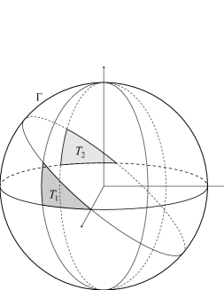
Figure 1: $\Omega={\mathbb{S}}^{2}-(T_{1}\cup T_{2})$ does not satisfies the condition (C1) when $\partial T_{1}=A_{1}\cup A_{2}\cup A_{3}$ and $\partial T_{2}=B_{1}\cup B_{2}\cup B_{3}$.

Before ending this section, let us give a result which is the converse of statement $(iii)$ in Lemma 2.5.

Lemma 3.6.

Let $u$ be a minimal graph on a domain $\Omega\subset{\mathbb{M}}^{2}$. Let $T\subset\partial\Omega$ be a geodesic arc such that $F_{u}(T)=|T|$ (resp. $F_{u}(T)=-|T|$). Then $u$ takes on $T$ the boundary value $+\infty$ (resp $-\infty$).

Let us consider $p\in T$, and $\Omega^{\prime}$ be the set of points in $\Omega$ at distance less than $\delta$ from $p$ ($\delta$ is chosen very small), $\Omega^{\prime}$ is a half-disk. Let $T^{\prime}$ be $T\cap\partial\Omega^{\prime}$, we have $F_{u}(T^{\prime})=|T^{\prime}|$ and the other part of $\partial\Omega^{\prime}$ is strictly convex. From Theorem 3.3, there exists on $\Omega^{\prime}$ a minimal graph $v$ with $u=v$ on $\partial\Omega^{\prime}\backslash T^{\prime}$ and $v=+\infty$ on $T^{\prime}$. The lemma is proved if we show that $u=v$.

If the lemma is not true, we can assume that $\{u<v-\varepsilon\}$ is nonempty; where $\varepsilon$ is chosen to be a regular value of $v-u$. Let $O$ denote $\{u<v-\varepsilon\}$. Let $C$ be the connected component of the complement of $O$ which has $\partial\Omega^{\prime}\backslash T^{\prime}$ in its boundary and we consider $O^{\prime}$ the complement of $C$: we have $O\subset O^{\prime}$ and $\partial O^{\prime}\subset\partial O\cup T^{\prime}$. Let $q$ be a point in $\partial O^{\prime}\cap\Omega^{\prime}$. For $\mu>0$, let $O^{\prime}(\mu)$ be the set of point $O^{\prime}$ at distance larger than $\mu$ from $T^{\prime}$. Let $q_{1}$ and $q_{2}$ be the endpoints of the connected component of $\partial O^{\prime}(\mu)\cap\partial O^{\prime}$ which contains $q$. Let $p_{i}$ be the projection of $q_{i}$ on $T^{\prime}$. Let $\widetilde{O}(\mu)$ be the domain bounded by the segments $[q_{1},p_{1}]$, $[p_{1},p_{2}]\subset T^{\prime}$, $[p_{2},q_{2}]$ and the boundary component of $O^{\prime}(\mu)$ between $q_{2}$ and $q_{1}$. On this last component $\Gamma(\mu)$ the vector $X_{u}-X_{v}$ points outside $\widetilde{O}(\mu)$. Since $F_{u}(\partial\widetilde{O}(\mu))=0=F_{v}(\partial\widetilde{O}(\mu))$, we have:

$$0<\int_{\Gamma(\mu)}\langle X_{u}-X_{v},\nu\rangle =-\int_{[p_{1},q_{1}]\cup[p_{2},q_{2}]}\langle X_{u}-X_{v},\nu\rangle-\int_{[p_{1},p_{2}]}\langle X_{u}-X_{v},\nu\rangle$$

$$\leq 4\mu-\int_{[p_{1},p_{2}]}\langle X_{u}-X_{v},\nu\rangle$$

By hypothesis on $u$ and $v$ and Lemma 2.5$-(iii)$, the last term vanishes; moreover the integral on $\Gamma(\mu)$ increases as $\mu$ goes to $0$ (see Lemma 2 in [2]). Thus we have a contradiction and $u=v$.

4 A particular case: ${\mathbb{M}}={\mathbb{H}}^{2}$

In the rest of the paper we study the Dirichlet problem for unbounded domains in ${\mathbb{H}}^{2}$.

Collin and Rosenberg [3] have extended Theorems 2.8 and 2.9 to some unbounded domains. More precisely, they consider simply connected domains $\Omega\subset{\mathbb{H}}^{2}$ whose boundary consists of finitely many ideal geodesics and finitely many complete convex arcs (convex towards $\Omega$) together with their endpoints at infinity, $\Omega$ satisfying the following assumption:

Figure 2: A domain $\Omega\subset{\mathbb{H}}^{2}$ satisfying condition (C-R).

(C-R) If $C\subset\partial\Omega$ is a convex arc with endpoint $p\in\partial_{\infty}{\mathbb{H}}^{2}$, then the other arc $\gamma$ of $\partial\Omega$ having $p$ as an endpoint is asymptotic to $C$ at $p$; i.e., if $\{x_{n}\}$ is a sequence in $\gamma$ converging to $p$, then ${\rm dist}_{{\mathbb{H}}^{2}}(x_{n},C)\to 0$ (see Figure 2).

They solve the Dirichlet problem for such domains. The same results without assuming $\Omega$ is simply connected can be obtained from Theorem 3.3, following Collin and Rosenberg’s ideas. Our aim is to weaken the hypotheses on $\Omega$, in particular the (C-R) hypothesis. Also we will allow $\Omega$ to have arcs in $\partial_{\infty}{\mathbb{H}}^{2}$ in its closure.

4.1 Minimal graphs over unbounded domains

4.1.1 First examples

Let $p$ be a point in $\partial_{\infty}{\mathbb{H}}^{2}$. We consider the half-plane model for the hyperbolic plane, ${\mathbb{H}}^{2}=\{(x,y)\in{\mathbb{R}}^{2}\ |\ y>0\}$ with metric $\langle\ ,\ \rangle=\frac{1}{y^{2}}\,g_{0}$, where $g_{0}$ is the Euclidean metric and assume that $p$ is the point of coordinates $(0,0)$. For $(\phi,\theta)\in{\mathbb{R}}\times(0,\pi)$ we consider the point $q=(e^{\phi}\cos\theta,e^{\phi}\sin\theta)\in{\mathbb{R}}\times{\mathbb{R}}_{+}^{*}={\mathbb{H}}^{2}$. We will call $(\phi,\theta)$ the polar coordinates of $q$ centered at $p$. In these new coordinates, the hyperbolic metric becomes $\frac{1}{\sin^{2}\theta}(d\phi^{2}+d\theta^{2})$; the coordinates $(\phi,\theta)$ are conformal.

We notice that there are several polar coordinates centered at $p$ i.e. given a point $q\in{\mathbb{H}}^{2}$ there exists one hyperbolic isometry fixing $p$ such that the polar coordinates centered at $p$ of $q$ becomes $(0,\pi/2)$. The curves $\{\phi=constant\}$ are geodesics. The curve $\{\theta=\pi/2\}$ is also a geodesic of ${\mathbb{H}}^{2}$ and, for any $\theta_{0}\in(0,\pi)$, the curve $\{\theta=\theta_{0}\}$ is equidistant to this geodesic; we denote by

$$d_{\theta_{0}}=\left|\int_{\theta_{0}}^{\pi/2}\frac{d\theta}{\sin\theta}\right|$$ (2)

the distance between the geodesic $\{\theta=\pi/2\}$ and its equidistant $\{\theta=\theta_{0}\}$.

A minimal graph $u$ which takes constant values on the equidistant curves to the geodesic $\{\theta=\pi/2\}$ can be written $u(\phi,\theta)=f(\theta)$, where $f$ satisfies the following differential equation (see Appendix A):

$$\dfrac{d}{d\theta}\left(\frac{f^{\prime}}{\sqrt{1+\sin^{2}\theta\left|f^{\prime}\right|^{2}}}\right)=0$$

Thus, by integrating this equation with $f(0)=0$, we get minimal surfaces that were first obtained by Sa Earp [15] and Abresch (see Appendix A).

Lemma 4.1.

Let $\theta_{0}\in(0,\pi/2]$. There is a minimal graph $h_{\theta_{0}}$ defined on the domain $\Omega_{\theta_{0}}=\{0<\theta<\theta_{0}\}$ which takes constant values on the equidistant curves to $\{\theta=\pi/2\}$, have boundary data $0$ on the boundary arc $\{\theta=0\}$ and satisfies $\dfrac{dh_{\theta_{0}}}{d\nu}=+\infty$ on $\{\theta=\theta_{0}\}$ ($\nu$ is the outer unit normal to $\partial\Omega_{\theta_{0}}$). When $\theta_{0}<\pi/2$, $h_{\theta_{0}}$ takes a constant finite value on $\{\theta=\theta_{0}\}$ and $h_{\pi/2}$ diverges to $+\infty$ on the geodesic $\{\theta=\pi/2\}$

In the half-plane model, the minimal graph $h_{\pi/2}$ is defined on ${\mathbb{R}}_{+}^{*}\times{\mathbb{R}}_{+}^{*}$ by

$$h_{\pi/2}(x,y)=\ln\frac{\sqrt{x^{2}+y^{2}}+y}{x}$$ (3)

Then if $\Omega$ is a domain bounded by a geodesic and an arc in $\partial_{\infty}{\mathbb{H}}^{2}$, Lemma 4.1 gives a minimal graph $h$ over $\Omega$ with value $0$ on the arc in $\partial_{\infty}{\mathbb{H}}^{2}$ and $h=+\infty$ on the geodesic. We notice that $\pm h+M$ is a minimal graph over $\Omega$ with value $M$ on the arc in $\partial_{\infty}{\mathbb{H}}^{2}$ and $\pm\infty$ on the geodesic. These minimal graphs are examples of solutions to a Dirichlet problem that can be recovered by the work of Collin and Rosenberg in [3].

In the following, we want to generalize such examples. The above surfaces will be used as barriers to study boundary values and uniqueness. As above, the domains $\Omega$ we shall study have arcs in $\partial_{\infty}{\mathbb{H}}^{2}$ as boundary; thus we shall denote by $\partial\Omega$ the boundary of $\Omega$ in ${\mathbb{H}}^{2}$ and by $\partial_{\infty}\Omega$ the boundary of $\Omega$ in the compactified space ${\mathbb{H}}^{2}\cup\partial_{\infty}{\mathbb{H}}^{2}$; $\overline{\Omega}^{\infty}$ will denote the closure of $\Omega$ in ${\mathbb{H}}^{2}\cup\partial_{\infty}{\mathbb{H}}^{2}$.

4.1.2 Convergence of sequences of minimal graphs

In this section, we solve the Dirichlet problem in a more general setting, where a maximum principle is not necessarily satisfied (see Section 4.3). We cannot then apply the method developed by Jenkins and Serrin to solve the Dirichlet problem on $\Omega$, since we cannot assure the monotonicity of the constructed graphs $u_{n}$ in the third step of the proof (see the third case “$\{C_{i}\}\neq\emptyset$” in the proof of Theorem 3.3). We now study the convergence of a (non necessarily monotone) sequence of minimal graphs on $\Omega$.

Let $\Omega\subset{\mathbb{H}}^{2}$ be a domain whose boundary $\partial_{\infty}\Omega$ is piecewise smooth (possibly with some arcs at $\partial_{\infty}{\mathbb{H}}^{2}$). Given a sequence $\{u_{n}\}$ of minimal graphs on $\Omega$, we define the convergence domain of the sequence $\{u_{n}\}$ as

$${\cal B}=\left\{p\in\Omega\ |\ \{|\nabla u_{n}(p)|\}\text{ is bounded}\right\},$$

and the divergence set of $\{u_{n}\}$ as

$${\cal D}=\Omega-{\cal B}.$$

We remark that, in Theorem 2.2, we have already defined a notion of convergence and divergence set for monotone sequences. In the following, we only use these new definitions.

The following lemma gives us a local description of the convergence domain ${\cal B}$ and the divergence set ${\cal D}$ that justifies their names. $G(u_{n})$ will denote the graph of $u_{n}$, and $N_{n}(p)$ the downward pointing normal vector to $G(u_{n})$ at the point $(p,u_{n}(p))$; i.e. $N_{n}=(X_{u_{n}},\frac{-1}{W_{u_{n}}})$. For writting this, we use a vertical translation to identify the tangent space $T({\mathbb{H}}^{2}\times{\mathbb{R}})$ with $T{\mathbb{H}}^{2}\times{\mathbb{R}}$. In fact, in the following, we often use vertical translations to identify the tangent spaces.

Lemma 4.2.

1. Given $p\in{\cal B}$, there exists a subsequence of $\{u_{n}-u_{n}(p)\}$ converging uniformly to a minimal graph in a neighborhood of $p$ in $\Omega$. The size of the neighborhood depends only on the distance from $p$ to $\partial\Omega$ and an upper-bound for $\{|\nabla u_{n}(p)|\}$. Also, ${\cal B}$ open follows from curvature estimates.

2. If $p\in{\cal D}$, there exists a compact geodesic arc $L_{p}(\delta)\subset\Omega$ of length $2\delta$ centered at $p$, $\delta>0$ only depends on ${\rm dist}_{{\mathbb{H}}^{2}}(p,\partial\Omega)$, such that, after passing to a subsequence, $\{N_{n}(q)\}$ converges to a horizontal vector orthogonal to $L_{p}(\delta)$ at every point $q\in L_{p}(\delta)$.

Fix $p\in\Omega$, and define $v_{n}=u_{n}-u_{n}(p)$. We denote by $G(v_{n})$ the graph of $v_{n}$. Observe that, for any $q\in\Omega$, the downward pointing normal vector to $G(v_{n})$ at $Q=(q,v_{n}(q))$ coincides with $N_{n}(q)$, and that both the convergence and divergence sets associated to $\{v_{n}\}$ and $\{u_{n}\}$ coincide. The distance from $P=(p,0)$ to the boundary of $G(v_{n})$ is bigger than or equal to $d={\rm dist}_{{\mathbb{H}}^{2}}(p,\partial\Omega)$. Hence we deduce from Schoen’s curvature estimates [16] that there exists $\delta>0$ depending on $d$ such that a neighborhood of $P=(p,0)$ in $G(v_{n})$ is a graph of uniformly bounded height and slope over the disk ${\mathbb{D}}_{n}(\delta)\subset T_{P}G(v_{n})$ of radius $\delta$ centered at the origin of $T_{P}G(v_{n})$ (see [13], Lemma 4.1.1, for more details). By graph here we mean a graph in geodesic coordinates, orthogonal to ${\mathbb{D}}_{n}(\delta)$. We call $G_{n}(p,\delta)$ such a graph.

Suppose $p\in{\cal B}$. Since $\{|\nabla u_{n}(p)|\}$ is uniformly bounded, a subsequence of $\{N_{n}(p)\}$ converges to a non-horizontal vector, so the tangent planes $T_{P}G(v_{n})$ converge to a non-vertical plane $\Pi$, and the disks ${\mathbb{D}}_{n}(\delta)$ converge to a disk ${\mathbb{D}}(\delta)\subset\Pi$ of radius $\delta$. From standard arguments (see [13], Theorem 4.1.1) we deduce that a subsequence of $\{G_{n}(p,\delta)\}$ converges to a minimal graph $G(p,\delta)$ over ${\mathbb{D}}(\delta)$. Hence there exists a disk $D(p,\widetilde{\delta})\subset\Omega$ of radius $\widetilde{\delta}\in(0,\delta]$ such that $\{v_{n}|_{D(p,\widetilde{\delta})}\}$ is uniformly bounded. After passing to a subsequence, $\{v_{n}|_{D(p,\delta)}\}$ converges uniformly on compact subsets of $D(p,\widetilde{\delta})$ to a minimal (vertical) graph. This proves 1.

Now assume $p\in{\cal D}$. Since $\{|\nabla u_{n}(p)|\}$ is unbounded, we can take a subsequence of $\{u_{n}\}$ so that $|\nabla u_{n}(p)|\to+\infty$ and $\{N_{n}(p)\}$ converges to a horizontal vector. In particular, the tangent planes $T_{P}(G(v_{n}))$ converge to a vertical plane $\Pi$, and a subsequence of $\{G_{n}(p,\delta)\}$ converges to a minimal graph $G(p,\delta)$ over a disk ${\mathbb{D}}(\delta)\subset\Pi$ of radius $\delta$ centered at $P$. The graph $G(p,\delta)$ is tangent to $\Pi$ at $P$. The following argument follows the ideas in [7], Claim 1: If $G(p,\delta)\not\subset\Pi$, then $G(p,\delta)\cap\Pi$ consists of $k\geq 2$ smooth curves meeting transversally at $P$. In particular, there are parts of $G(p,\delta)$ on both sides of $\Pi$. Thus there are points in $G(p,\delta)$ where the normal vector points up and points where the normal points down. But this is impossible, since $G(p,\delta)$ is the limit of vertical graphs. Therefore, $G(p,\delta)\subset\Pi$.

We call $L_{p}(\delta)$ the geodesic $G(p,\delta)\cap({\mathbb{H}}^{2}\times\{0\})$, whose length is $2\delta$. We can deduce that the tangent planes of $G(v_{n})$ at $(q,v_{n}(q))$ converge to $\Pi$, for every $q\in L_{p}(\delta)$ (for precise details, see [9, 10]), which completes the proof of Lemma 4.2.

The next lemma shows ${\cal D}=\cup_{i\in I}L_{i}$, where each $L_{i}$ is a component of the intersection of a ideal geodesic in ${\mathbb{H}}^{2}$ with $\Omega$. The geodesics $L_{i}$ are called divergence lines.

Lemma 4.3.

Given $p\in{\cal D}$, there exists a geodesic $L\in\Omega$ joining points in $\partial_{\infty}\Omega$ (possibly at $\partial_{\infty}{\mathbb{H}}^{2}$) which passes through $p$ and such that, after passing to a subsequence, $\{N_{n}|_{L}\}$ converges to a horizontal vector orthogonal to $L$ (in particular, $L\subset{\cal D}$). In fact, $L$ is the geodesic containing $L_{p}(\delta)$.

Let $L_{p}=L_{p}(\delta)$ be the geodesic arc given in Lemma 4.2-2, and $L$ be the geodesic in $\Omega$ joining points in $\partial\Omega$ which contains $L_{p}$. For every $q$, we denote by $[p,q]\subset L$ the closed geodesic arc in $L$ joining $p,q$. Define

$$\Lambda=\left\{q\in L\ \Big{|}\ \begin{array}[]{ll}\mbox{ there exists a subsequence of }\{u_{n}\}\ \mbox{ such that }\\ N_{n}|_{[p,q]}\ \mbox{ becomes horizontal and orthogonal to }L\end{array}\right\}.$$

Clearly, $p\in\Lambda$ so $\Lambda\neq\emptyset$. Let us prove $\Lambda$ is open in $L$. Take $q\in\Lambda$, and denote by $\{u_{\sigma(n)}\}$ its associated subsequence given in the definition of $\Lambda$. Since $\Lambda\subset{\cal D}$, Lemma 4.2-2 gives us a geodesic arc $L_{q}$ through $q$ such that, passing to a subsequence, $N_{\sigma(n)}|_{L_{q}}$ becomes horizontal and orthogonal to $L_{q}$. The vector $N_{\sigma(n)}(q)$ converges to a horizontal vector orthogonal simultaneously to $L$ and $L_{q}$, from which we deduce that $L_{q}\subset L$, and so $L_{q}\subset\Lambda$.

Finally, we prove $\Lambda$ is a closed set, which finishes Lemma 4.3. Let $\{q_{m}\}$ be a sequence of points in $\Lambda$ such that $q_{m}\to q\in L$. Let us prove that $q\in\Lambda$. For each $m$, there exists a subsequence of $\{u_{n}\}$ such that $N_{n}|_{[p,q_{m}]}$ becomes horizontal and orthogonal to $L$. A diagonal argument allows us to take a common subsequence of $\{u_{n}\}$ (also denoted by $\{u_{n}\}$) such that $N_{n}|_{[p,q_{m}]}$ becomes horizontal and orthogonal to $L$, for every $m$. For every $m$, there is a geodesic arc $L_{q_{m}}\subset L$ centered at $q_{m}$ satisfying Lemma 4.2-2 whose length depends only on ${\rm dist}_{{\mathbb{H}}^{2}}(q_{m},\partial\Omega)$. Hence, $q\in L_{q_{m}}$ for any $m$ large enough, and so $q\in\Lambda$.

Proposition 4.4.

Suppose the divergence set of $\{u_{n}\}$ is a countable set of lines. Then there exists a subsequence of $\{u_{n}\}$ (denoted as the original sequence) such that:

1. The divergence set ${\cal D}$ of $\{u_{n}\}$ is composed of a countable number of divergence lines, pairwise disjoint.

2. For any component $\Omega^{\prime}$ of ${\cal B}=\Omega-{\cal D}$ and any $p\in\Omega^{\prime}$, $\{u_{n}-u_{n}(p)\}$ converges uniformly on compact sets of $\Omega^{\prime}$ to a minimal graph over $\Omega^{\prime}$.

Suppose $L_{1}$ is a divergence line of $\{u_{n}\}$. Lemma 4.2 assures that, passing to a subsequence, $\{N_{n}(q)\}$ converges to a horizontal vector orthogonal to $L_{1}$ at $q$, for each $q\in L_{1}$. Observe that the divergence set associated to such a subsequence (denoted again by $\{u_{n}\}$) is contained in the divergence set of the original sequence. In particular, the divergence set for such a subsequence, denoted by ${\cal D}$, contains a countable number of divergence lines.

Suppose there exists a divergence line $L_{2}\subset{\cal D}$, $L_{2}\neq L_{1}$. Passing to a subsequence, we obtain that $\{N_{n}(q)\}$ converges to a horizontal vector orthogonal to $L_{2}$, for each $q\in L_{2}$. In particular, $L_{1}\cap L_{2}=\emptyset$, since if there exists some $q\in L_{1}\cap L_{2}$ then $N_{n}(q)$ would converge to a horizontal vector orthogonal to both $L_{1},L_{2}$ simultaneously, a contradiction. The “new” divergence set ${\cal D}$ is then a countable set of divergence lines containing $L_{1}$ and $L_{2}$, with $L_{1}\neq L_{2}$.

Continuing the above argument, we obtain with a diagonal process a subsequence of $\{u_{n}\}$ (also denoted by $\{u_{n}\}$) whose divergence set ${\cal D}$ is composed of a countable number of pairwise disjoint divergence lines $L_{i}$.

Now consider a countable set of points $\{p_{i}\}_{i}$ dense in ${\cal B}$, the convergence domain associated to the subsequence obtained in the previous argument. Using Lemma 4.2-1 and a diagonal argument, we obtain a subsequence of $\{u_{n}\}$ such that $\{u_{n}-u_{n}(p)\}$ converges uniformly on compact sets of $\Omega^{\prime}$ to a minimal graph, for every component $\Omega^{\prime}$ of ${\cal B}$ and every $p\in\Omega^{\prime}$. This finishes the proof of Proposition 4.4.

Remark 4.5.

In Proposition 4.4 we can remove the hypothesis ${\cal D}$ is a countable set of divergence lines, and we obtain that, after passing to a subsequence, ${\cal D}$ is composed of pairwise disjoint divergence lines and, up to a vertical translation, we have uniform convergence on compact sets of each component of the convergence domain ${\cal B}$. The proof of this fact is more involved and will be included in [4].

We will only use Proposition 4.4 in the case the divergence set ${\cal D}$ is composed of a finite number of divergence lines.

Let $\{u_{n}\}$ be a subsequence given by Proposition 4.4. We consider $\Omega^{\prime}$ a connected component of $\mathcal{B}$. Its boundary is composed of subarcs of $\partial\Omega$ and divergence lines. Let us understand the limit $u$ of $\{u_{n}-u_{n}(p)\}$ in $\Omega^{\prime}$ ($p\in\Omega^{\prime}$). Let $T$ be a subarc of $\partial\Omega^{\prime}$ included in a divergence line. From the convergence of $\{N_{n}\}$ along $T$, $F_{u_{n}}(T)$ converges to $\pm|T|$. Since $|X_{u_{n}}|$ is bounded by $1$, this implies that $F_{u}(T)=\pm|T|$. Then by Lemma 3.6, $u$ takes value $\pm\infty$ on $T$. In fact we have a stronger result.

Lemma 4.6.

Let $\{u_{n}\}$ be a sequence of minimal graphs on $\Omega$. We assume that $\{u_{n}\}$ converges to a minimal graph $u$ on a connected subdomain $\Omega^{\prime}$ of $\Omega$. Let $T$ be a subarc in $\partial\Omega^{\prime}$ included in a divergence line for the sequence $\{u_{n}\}$ such that $X_{u_{n}}\rightarrow\nu$ along $T$ with $\nu$ the outgoing normal to $\Omega^{\prime}$. Then if $p\in\Omega^{\prime}$ and $q\in T$ we have

$$\lim_{n\rightarrow+\infty}u_{n}(q)-u_{n}(p)=+\infty$$

Since $X_{u_{n}}\rightarrow\nu$ on $T$, $F_{u_{n}}(T)$ converges to $|T|$. Thus $u$ takes the value $+\infty$ on $T$. Let $p$ and $q$ be as in the lemma and consider the disk model for ${\mathbb{H}}^{2}$ assuming that $q$ is at the origin, $T$ is a subarc of $\{x=0\}$ and $\nu$ points to the half-plane $\{x\geq 0\}$. Let us prove:

$$\text{There is }\epsilon>0\text{ such that }\dfrac{\partial u_{n}}{\partial x}>0\text{ on }\{-\epsilon<x\leq 0,y=0\}\text{ for large }n. *$$ ()

Since $u=+\infty$ on $T$ there is $\epsilon>0$ such that $\dfrac{\partial u}{\partial x}\geq 1$ on $\{-\epsilon<x<0,y=0\}$. The convergence $u_{n}\rightarrow u$ implies : for every $0<\eta<\epsilon$, $\dfrac{\partial u_{n}}{\partial x}>0$ on $\{-\epsilon<x<-\eta,y=0\}$ for large $n$. If ($*$ ‣ 4.1.2) is not true, considering a subsequence if necessary, there is $q_{n}$ in $\{-\epsilon<x\leq 0,y=0\}$ with $\dfrac{\partial u_{n}}{\partial x}(q_{n})=0$. Observe that it must be $q_{n}\rightarrow q$.

If the sequence $\{|\nabla u_{n}(q_{n})|\}$ is bounded, $|\nabla u_{n}|$ is uniformly bounded in a uniform disk around $q_{n}$. Since $q_{n}\rightarrow q$, the sequence $\{|\nabla u_{n}(q)|\}$ is bounded which is false since $q$ lies on a divergence line. Hence, passing to a subsequence, we can assume that $|\nabla u_{n}(q_{n})|\rightarrow+\infty$. Let $D_{n}^{1}$ be the $\delta$-geodesical disk centered at $(q_{n},0)$ in the graph of $u_{n}-u_{n}(q_{n})$ ($\delta$ is fixed small enough with respect to the distance from $q$ to $\partial\Omega$). Since $\dfrac{\partial u_{n}}{\partial x}(q_{n})=0$ we can prove as in Lemma 4.2 that the sequence $\{D_{n}^{1}\}$ converges to the vertical disk in $\{y=0\}\times{\mathbb{R}}$ centered at $(q,0)$ of radius $\delta$. Let $D_{n}^{2}$ be the $\delta$-geodesical disk centered at $(q,0)$ in the graph of $u_{n}-u_{n}(q)$. Since $T$ is part of a divergence line, $\{D_{n}^{2}\}$ converges to the vertical disk in $\{x=0\}\times{\mathbb{R}}$ centered at $(q,0)$ or radius $\delta$. Because of both convergences, for large $n$, $D_{n}^{1}$ and $D_{n}^{2}$ intersect transversally. But this is impossible, since their normal vectors at a point depends only on $\nabla u_{n}$.

Assertion ($*$ ‣ 4.1.2) is then proved. Let $q_{t}$ be the point of coordinates $(-t,0)$. Since $u$ takes the value $+\infty$ at $q$ we can make $u(q_{t})-u(p)$ as large as we want by taking $t$ small . Besides, for large $n$, ($*$ ‣ 4.1.2) gives $u_{n}(q)-u_{n}(p)\geq u_{n}(q_{t})-u_{n}(p)$. Since $u_{n}\rightarrow u$, we get $u_{n}(q)-u_{n}(p)\geq u(q_{t})-u(p)-1$. This proves the lemma.

Remark 4.7.

Let $L$ be a divergence line and suppose there exist two components $\Omega_{1},\Omega_{2}$ of ${\cal B}$ such that $L\subset\partial\Omega_{i}$, $i=1,2$. Consider points $p_{1}\in\Omega_{1},\ p_{2}\in\Omega_{2}$. Passing to a subsequence, $\{u_{n}-u_{n}(p_{i})\}$ converges uniformly on compact sets of $\Omega_{i}$ to a minimal graph $u_{i}:\Omega_{i}\to{\mathbb{R}}$. Assume $F_{u_{1}}(T)=|T|$ for each bounded arc $T\subset L$, when $L$ is oriented as $\partial\Omega_{1}$. Then $F_{u_{2}}(T)=-|T|$, when $L$ is oriented as $\partial\Omega_{2}$. We deduce from Lemma 4.6 that $\{(u_{n}-u_{n}(p_{1}))|_{L}\}$ diverges to $+\infty$ and $\{(u_{n}-u_{n}(p_{2}))|_{L}\}$ diverges to $-\infty$. In particular, we can deduce that $\{u_{n}-u_{n}(p_{1})\}$ diverges uniformly on compact sets of $\Omega_{2}$ to $+\infty$.

Now, we are going to exclude the existence of some divergence lines under additional constraints. In particular, if there exists minimal graphs $w^{+},w^{-}$ defined on a neighborhood ${\cal U}\subset\overline{\Omega}$ of a point $p\in\partial\Omega$ such that $w^{-}\leq u_{n}\leq w^{+}$ for every $n$, then a divergence line cannot arrive at $p$. We will state conditions for which such barriers exist.

Proposition 4.8.

Let $\{u_{n}\}$ be the subsequence given by Proposition 4.4.

1. Let $C\subset\partial_{\infty}\Omega$ be a smooth arc where each $u_{n}$ extends continuously and suppose $\{u_{n}|_{C}\}$ converges to a continuous function $f$. Then a divergence line $L_{i}$ cannot finish at an interior point of $C$.

2. For every $n$, suppose there exists $M_{n}\geq 0$ such that $|u_{n}|\leq M_{n}$, and let $T\subset\partial\Omega$ be a bounded geodesic arc where $u_{n}$ extends continuously and $u_{n}|_{T}=M_{n}$ or $-M_{n}$. Then a divergence line cannot finish at an interior point of $T$.

Let $C\subset\partial_{\infty}\Omega$ be an arc as in item 1. Suppose $C$ is either an arc at $\partial_{\infty}{\mathbb{H}}^{2}$ or a strictly convex arc (with respect to $\Omega$). Let $p\in C$ and $C^{\prime}$ be a neighborhood of $p$ in $C$ such that $\overline{C^{\prime}}\subset C$. Consider the geodesic $\Gamma(C^{\prime})\subset{\mathbb{H}}^{2}$ joining the endpoints of $C^{\prime}$, and define the domain $\Delta\subset{\mathbb{H}}^{2}$ bounded by $C^{\prime}\cup\overline{\Gamma(C^{\prime})}$. For $C^{\prime}$ small enough, we can assume $\Delta\subset\Omega$.

Define $M=\max_{C^{\prime}}|f|$. For $n$ big enough and $C^{\prime}$ small enough, $|u_{n}|<M+1$ on $C^{\prime}$, for every $n$. Consider $w^{+},w^{-}:\Delta\to{\mathbb{R}}$ minimal graphs with boundary values

$$\left\{\begin{array}[]{ll}w^{+}=M+1&\mbox{, on }C^{\prime}\\ w^{+}=+\infty&\mbox{, on }\Gamma(C^{\prime})\end{array}\right.\qquad\left\{\begin{array}[]{ll}w^{-}=-M-1&\mbox{, on }C^{\prime}\\ w^{-}=-\infty&\mbox{, on }\Gamma(C^{\prime})\end{array}\right.$$

(they exist by Lemma 4.1 and Theorem 3.3, depending on the case). By the general maximum principle, $w^{-}\leq u_{n}\leq w^{+}$ for every $n$. Therefore, the Compactness Theorem says $\Delta\subset{\cal B}$, and so no divergence line finishes at $p$.

Now suppose that $C$ is geodesic and $u_{n}|_{C}=c\in{\mathbb{R}}$ for every $n$. We can assume without loss of generality $c=0$. By reflecting the graph surface of $u_{n}$ about $C$, we obtain a minimal surface $\Sigma$ containing $C$, whose normal vector along $C$ is orthogonal to $C$. If there exists a divergence line $L$ with an endpoint at $p\in C$, then we conclude $N_{n}(p)$ converges to a horizontal vector orthogonal to $L$. But this is impossible, since such a vector must be orthogonal to $C$. Hence, no divergence line finishes at $C$.

Finally, suppose $C$ is geodesic and there exists a divergence line $L$ with endpoint $p\in C$. Fix $\varepsilon>0$. Since $\{u_{n}|_{C}\}$ converges to a continuous function $f$, there exists a small neighborhood $C^{\prime}\subset C$ of $p$ such that $|u_{n}(q)-f(p)|<\varepsilon$, for every $q\in C^{\prime}$ and $n$ large enough. Consider a neighborhood ${\cal U}\subset\Omega\cup C$ of $p$ containing $C^{\prime}$, and define $v_{n}:{\cal U}\to{\mathbb{R}}$ as the minimal graph with boundary values

$$\left\{\begin{array}[]{ll}v_{n}=f(p)&\mbox{, in }C^{\prime}\\ v_{n}=u_{n}&\mbox{, in }\partial{\cal U}-C^{\prime}\end{array}\right.$$

(it exists by Theorem 3.3). The general maximum principle for bounded domains assures

$$u_{n}-\varepsilon\leq v_{n}\leq u_{n}+\varepsilon.$$ (4)

Next we prove that $L\cap{\cal U}$ is a divergence line for $\{v_{n}\}$, conveniently choosing $\varepsilon$ and ${\cal U}$. Fix a point $q\in L\cap{\cal U}$. From the proof of Lemma 4.2, we deduce there exists a neighborhood of $(q,0)$ in the graph $G(u_{n}-u_{n}(q))$ converging to the disk $D_{L}(q,\delta)\subset L\times{\mathbb{R}}$ of radius $\delta$ centered at $(q,0)$. Taking $\varepsilon\leq\delta/2$, we conclude using (4) that a neighborhood of the point $(q,v_{n}(q)-u_{n}(q))$ in $G(v_{n}-u_{n}(q))$ converges to $D_{L}(q,\delta)$, and $L\cap{\cal U}$ is a divergence line for $\{v_{n}\}$ (see [9], Proposition 1.4.8, for a detailed proof). But we know from the above argument this is not possible, as $v_{n}$ is constant on $C^{\prime}$. This finishes item 1.

Now, consider $T$ as in the hypothesis of 2, and let $p\in T$. Define $v_{n}=u_{n}-u_{n}(p)$ for every $n$. Clearly, $v_{n}|_{T}=0$ for every $n$. Then we obtain from item 1 that a divergence line for $\{v_{n}\}$ cannot finish at $T$. Since the divergence lines associated to $\{u_{n}\}$ coincide with those of $\{v_{n}\}$, we have proved Proposition 4.8.

4.1.3 Solving the Jenkins-Serrin problem on unbounded domains

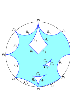
Figure 3: An ideal Scherk domain.

Let $\Omega\subset{\mathbb{H}}^{2}$ be a domain whose boundary $\partial_{\infty}\Omega$ consists of a finite number of geodesic arcs $A_{i},B_{i}$, a finite number of convex arcs $C_{i}$ (convex towards $\Omega$) and a finite number of open arcs $D_{i}$ at $\partial_{\infty}{\mathbb{H}}^{2}$, together with their endpoints, which are called the vertices of $\Omega$ (see Figure 3). We mark the $A_{i}$ edges by $+\infty$, the $B_{i}$ edges by $-\infty$, and assign arbitrary continuous data $f_{i},g_{i}$ on the arcs $C_{i},D_{i}$, respectively. Assume that no two $A_{i}$ edges and no two $B_{i}$ edges meet at a convex corner. We will call such a domain $\Omega$ an ideal Scherk domain.

A polygonal domain $\mathcal{P}$ is said to be inscribed in $\Omega$ if ${\mathcal{P}}\subset\Omega$ and its vertices are among the endpoints of the arcs $A_{i},B_{i},C_{i}$ and $D_{i}$; we notice that a vertex may be in $\partial_{\infty}{\mathbb{H}}^{2}$ and an edge may be one of the $A_{i}$ or $B_{i}$ (see Figure 4).

For each ideal vertex $p_{i}$ of $\Omega$ at $\partial_{\infty}{\mathbb{H}}^{2}$, we consider a horocycle $H_{i}$ at $p_{i}$. Assume $H_{i}$ is small enough so that it does not intersect bounded edges of $\partial\Omega$ and $H_{i}\cap H_{j}=\emptyset$ for every $i\neq j$. Given a polygonal domain ${\cal P}$ inscribed in $\Omega$, we denote by $\Gamma({\cal P})$ the part of $\partial{\cal P}$ outside the horocycles, and (see Figure 4)

$$\gamma=|\Gamma({\cal P})|,\qquad\alpha=\sum_{i}|A_{i}\cap\Gamma({\cal P})|\qquad{\rm and}\qquad\beta=\sum_{i}|B_{i}\cap\Gamma({\cal P})|.$$

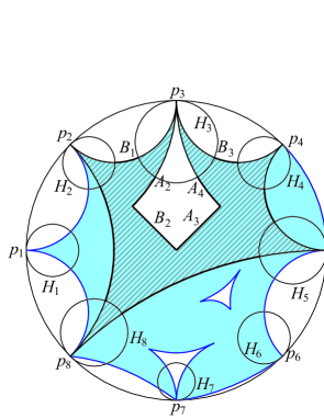
Figure 4: An inscribed polygonal domain in $\Omega$

Theorem 4.9.

If there is at least one edge $C_{i}$ or $D_{i}$ in $\partial_{\infty}\Omega$, then a solution to the Dirichlet problem on $\Omega$ exists if and only if the horocycles $H_{i}$ can be chosen so that

$$2\alpha<\gamma\qquad\mbox{and }\qquad 2\beta<\gamma$$ (5)

for every polygonal domain ${\cal P}$ inscribed in $\Omega$.

Remark 4.10.

If these conditions hold for some choice of horocycles, then they also holds for all smaller horocycles.

Given a vertex $p_{i}\in\partial_{\infty}{\mathbb{H}}^{2}$ of $\Omega$, we consider a sequence of nested horocycles $\{H_{i,n}\}$ converging to $p_{i}$. Assume $H_{i,n}\cap H_{j,n}=\emptyset$, for every $i\neq j$. Denote by ${\cal H}_{i,n}$ the horodisk bounded by $H_{i,n}$. Given an inscribed polygonal domain ${\cal P}\subset\Omega$, we call ${\cal P}_{n}$ the domain bounded by $\partial{\cal P}-\cup_{i}{\cal H}_{i,n}$ together with geodesic arcs contained in ${\cal P}\cap\left(\cup_{i}{\cal H}_{i,n}\right)$ joining points in $\partial{\cal P}\cap\left(\cup_{i}H_{i,n}\right)$. Define

$$\gamma_{n}=|\partial{\cal P}-\cup_{i}{\cal H}_{i,n}|,\qquad\alpha_{n}=\sum_{i}|A_{i}\cap\partial{\cal P}_{n}|,\qquad\beta_{n}=\sum_{i}|B_{i}\cap\partial{\cal P}_{n}|.$$

Observe that both sequences $\{2\alpha_{n}-\gamma_{n}\}$ and $\{2\beta_{n}-\gamma_{n}\}$ are monotonically decreasing.

Let us first prove the conditions are necessary in Theorem 4.9. Assume there exists a solution $u$ to the Dirichlet problem on $\Omega$, and let ${\cal P}\subset\Omega$ be an inscribed polygon. Since either $\{C_{i}\}\neq\emptyset$ or $\{D_{i}\}\neq\emptyset$, there exists a curve $\eta\subset\partial{\cal P}$ which is not an $A_{i}$ or $B_{i}$ edge. Let $\widetilde{\eta}\subset\eta$ be a fixed bounded arc. Lemma 2.5 assures $F_{u}(\partial{\cal P}_{n})=0$, $\sum_{i}F_{u}(A_{i}\cap\partial{\cal P}_{n})=\alpha_{n}$ and $|F_{u}(\partial{\cal P}_{n}\setminus(\cup_{i}A_{i}\cup\widetilde{\eta}))|\leq\gamma_{n}-\alpha_{n}-|\widetilde{\eta}|$. Thus we obtain

$$\alpha_{n}\leq\gamma_{n}-\alpha_{n}-|\widetilde{\eta}|+|F_{u}(\widetilde{\eta})|+\varepsilon_{n},$$

where $\varepsilon_{n}=|\partial{\cal P}_{n}-\partial{\cal P}|$. This is, $2\alpha_{n}-\gamma_{n}<\varepsilon_{n}-(|\widetilde{\eta}|-|F_{u}(\widetilde{\eta})|)$. Analogously,

$$2\beta_{n}-\gamma_{n}<\varepsilon_{n}-(|\widetilde{\eta}|-|F_{u}(\widetilde{\eta})|).$$

Since $|F_{u}(\widetilde{\eta})|<|\widetilde{\eta}|$ (again by Lemma 2.5) and $\varepsilon_{n}$ converges to zero as $n$ goes to $+\infty$, then $\varepsilon_{n}<(|\widetilde{\eta}|-F_{u}(\widetilde{\eta}))$ for $n$ big enough. Therefore, condition (5) is satisfied for ${\cal P}$ and the horocycles $H_{i,n}$, for $n$ large enough.

Finally, observe there are a finite number of inscribed polygonal domains ${\cal P}$ in $\Omega$ (there are a finite number of vertices of $\Omega$). Thus we can choose $H_{i}=H_{i,n}$ for $n$ large so that (5) is satisfied for any inscribed polygonal domain ${\cal P}\subset\Omega$.

Let us now prove the conditions are sufficient. We choose $H_{i,1}=H_{i}$. Thus we have $2\alpha_{n}<\gamma_{n}$ and $2\beta_{n}<\gamma_{n}$ for every $n$.

We now construct domains $\Omega_{n}$ converging to $\Omega$. For any vertex $p_{i}\in\partial_{\infty}{\mathbb{H}}^{2}$ of $\Omega$, we consider a sequence of nested ideal geodesics $\Gamma_{i,n}$ converging to $p_{i}$. By nested we mean that, if $\Delta_{i,n}$ is the component of ${\mathbb{H}}^{2}\backslash\Gamma_{i,n}$ containing $p_{i}$ at its ideal boundary, then $\Delta_{i,n+1}\subset\Delta_{i,n}$. Assume $\Gamma_{i,n}\cap\Gamma_{j,n}=\emptyset$, for every $i\neq j$, and define

$$A_{i,n}=A_{i}\setminus\cup_{k}\Delta_{k,n},\quad B_{i,n}=B_{i}\setminus\cup_{k}\Delta_{k,n}\quad\mbox{ and}\quad C_{i,n}=C_{i}\setminus\cup_{k}\Delta_{k,n}.$$

For $r>0$ big enough, the annulus bounded by $\partial_{\infty}{\mathbb{H}}^{2}$ and the circle ${\mathbb{S}}_{{\mathbb{H}}^{2}}(0,r)$ of radius $r$ (in the hyperbolic metric) centered at the origin of the Poincaré disk, does not intersect the bounded components of $\partial\Omega$. Consider a monotone increasing sequence of radii $\{r_{n}\}$ converging to $+\infty$. For $r_{n}$ big enough, we can assume ${\mathbb{S}}_{{\mathbb{H}}^{2}}(0,r_{n})$ intersects every geodesic $\Gamma_{k,n}$ twice, and define by $D_{i,n}$ the component of ${\mathbb{S}}_{{\mathbb{H}}^{2}}(0,r)\setminus\cup_{k}\Delta_{k,n}$ converging to $D_{i}$. We can naturally assign the values $g_{i}$ on each $D_{i,n}$. Finally, let us call $\Omega_{n}$ the domain bounded by the edges $A_{i,n},B_{i,n},C_{i,n},D_{i,n}$, and the corresponding geodesic arcs $\Gamma_{i,n}^{j}\subset\Gamma_{i,n}$, together with their endpoints.

Figure 5: Construction of the domain $\Omega_{n}$

Theorem 3.3 assures, for each $m\in{\mathbb{N}}$, the existence of a unique minimal graph $u_{m}^{n}:\Omega_{n}\to{\mathbb{R}}$ with boundary values

$$\left\{\begin{array}[]{ll}u_{m}^{n}=m&\mbox{, on the }A_{i,n}\mbox{ edges.}\\ u_{m}^{n}=-m&\mbox{, on the }B_{i,n}\mbox{ edges.}\\ u_{m}^{n}=f_{i,m}&\mbox{, on the }C_{i,n}\mbox{ edges.}\\ u_{m}^{n}=g_{i,m}&\mbox{, on the }D_{i,n}\mbox{ edges.}\\ u_{m}^{n}=0&\mbox{, on the geodesic arcs }\Gamma_{i,n}^{j}.\end{array}\right.$$

where $f_{i,m}$ (resp. $g_{i,m}$) denotes the function $f_{i}$ (resp. $g_{i}$) truncated above and below by $m$ and $-m$, respectively. By the maximum principle for bounded domains, $-m\leq u_{m}^{n}\leq m$, for every $n$. Then we can extract, by using the compactness theorem and a diagonal argument, a subsequence of $\{u_{m}^{n}\}_{n}$ converging uniformly on compact subsets of $\Omega$ to a minimal graph $u_{m}:\Omega\to[0,m]$ with boundary data

$$\left\{\begin{array}[]{ll}u_{m}=m&\mbox{, on the }A_{i}\mbox{ edges.}\\ u_{m}=-m&\mbox{, on the }B_{i}\mbox{ edges.}\\ u_{m}=f_{i,m}&\mbox{, on the }C_{i}\mbox{ edges.}\\ u_{m}=g_{i,m}&\mbox{, on the }D_{i}\mbox{ edges.}\\ \end{array}\right.$$

Such boundary data are obtained from a standard barrier argument, using as barriers the ones described in [3].

We are going to prove that a subsequence of $\{u_{m}\}$ converges to a solution to the Dirichlet problem on $\Omega$, proving Theorem 4.9. We know from Proposition 4.8 that divergence lines for $\{u_{m}\}$ can only arrive at vertices of $\Omega$. In particular, there exists a finite number of divergence lines, and so ${\cal B}\neq\emptyset$.

Passing to a subsequence, we can assume $\{u_{n}\}$ satisfies Proposition 4.4. Now suppose by contradiction that ${\cal B}\neq\Omega$; i.e., suppose there exists a divergence line $L\subset{\cal D}$. We then deduce from Remark 4.7 there exists a component ${\cal P}\subset{\cal B}$ such that $\{u_{n}\}$ diverges uniformly on compact sets of ${\cal P}$, say to $+\infty$ (the case $-\infty$ follows similarly). Take a point $p\in{\cal P}$. Then $\{u_{n}-u_{n}(p)\}$ converges uniformly on compact subsets of ${\cal P}$ to a minimal graph $u:{\cal P}\to{\mathbb{R}}$. Observe that $u$ diverges to $-\infty$ as we approach any edge in $\partial{\cal P}\cap\left(\partial\Omega-\cup_{i}A_{i}\right)$ within ${\cal P}$. We then get ${\cal P}$ is a polygonal domain and $F_{u}(T)=-|T|$ for every bounded arc $T\subset\partial{\cal P}\cap\left(\partial\Omega-\cup_{i}A_{i}\right)$.

Claim 4.11.

We can choose the polygonal domain ${\cal P}\subset{\cal B}$ so that $F_{u}(T)=-|T|$ for any bounded geodesic arc $T\subset\partial{\cal P}-\cup_{i}A_{i}$.

Assume Claim 4.11 is true and define ${\cal P}_{n}$ as at the beginning of the proof. Thus $F_{u}(\partial{\cal P}_{n}-\cup_{i}A_{i}-(\partial{\cal P}_{n}-\partial{\cal P}))=-|\partial{\cal P}_{n}-\cup_{i}A_{i}-(\partial{\cal P}_{n}-\partial{\cal P})|$. By Lemma 2.5,

$$\left\{\begin{array}[]{l}\sum_{i}F_{u}(A_{i}\cap\partial{\cal P}_{n})+F_{u}(\partial{\cal P}_{n}-\partial{\cal P})\\ \mbox{}\\ \mbox{}\hskip 56.9055pt+F_{u}(\partial{\cal P}_{n}-\cup_{i}A_{i}-(\partial{\cal P}_{n}-\partial{\cal P}))=0,\\ \mbox{}\\ \left|\sum_{i}F_{u}(A_{i}\cap\partial{\cal P}_{n})+F_{u}(\partial{\cal P}_{n}-\partial{\cal P})\right|\leq\alpha_{n}+\varepsilon_{n},\end{array}\right.$$

where $\varepsilon_{n}=|\partial{\cal P}_{n}-\partial{\cal P}|$, which converges to zero as $n\to+\infty$. Hence,

$$\gamma_{n}-\alpha_{n}-\varepsilon_{n}\leq\alpha_{n}+\varepsilon_{n}.$$

Thus we obtain $-2\varepsilon_{n}\leq 2\alpha_{n}-\gamma_{n}\leq 2\alpha_{1}-\gamma_{1}$, for every $n$. Since $\varepsilon_{n}\to 0$ as $n\to+\infty$, we obtain a contradiction to the first condition in (5). (If we suppose there exists a component ${\cal P}\subset{\cal B}$ such that $\{u_{n}\}$ diverges uniformly to $-\infty$ on compact sets of ${\cal P}$, we similarly achieve a contradiction using that $2\beta_{1}-\gamma_{1}<0$). Hence there are no divergence lines for $\{u_{n}\}$, and so ${\cal B}=\Omega$.

Applying a flux argument as above, we obtain that $\{u_{n}\}$ converges uniformly on compact sets of $\Omega$ to a minimal graph $u:\Omega\to{\mathbb{R}}$. Finally, using barrier functions as in [3] or those defined in Lemma 4.1 for the $D_{i}$ edges, we deduce that $u$ takes the desired boundary values, and this proves Theorem 4.9.

So it only remains to prove Claim 4.11. Note we must only prove there exists a component ${\cal P}$ of ${\cal B}$ such that $\{u_{n}\}$ diverges to $+\infty$ uniformly on compact sets of ${\cal P}$ and $F_{u}(T)=-|T|$ for any bounded geodesic arc $T$ contained in a divergence line in $\partial{\cal P}$. Observe that, since ${\cal B}\neq\Omega$ is assumed, every component of ${\cal B}$ contains at least one divergence line in its boundary.

We know there exists a component ${\cal U}_{0}\subset{\cal B}$ which is an inscribed polygonal domain and such that $\{u_{n}\}$ diverges to $+\infty$ uniformly on compact sets of ${\cal U}_{0}$. If ${\cal U}_{0}$ satisfies Claim 4.11, we have finished. Otherwise, there exists a divergence line $L_{0}\subset\partial{\cal U}_{0}$ such that $F_{u_{n}}(L_{0})\to|L_{0}|$ with the orientation induced by $\partial{\cal U}_{0}$. Let ${\cal U}_{1}$ be the component of ${\cal B}$ different from ${\cal U}_{0}$ containing $L_{0}$ in its boundary. Hence $F_{u_{n}}(L_{0})\to-|L_{0}|$ when $L_{0}$ is oriented as $\partial{\cal U}_{1}$. We deduce from Remark 4.7 that $\{u_{n}\}$ diverges to $+\infty$ uniformly on compact sets of ${\cal U}_{1}$.

If ${\cal U}_{1}$ satisfies the conditions of Claim 4.11, we are done. Otherwise, there exists another divergence line $L_{1}\subset\partial{\cal U}_{1}$ such that $F_{u_{n}}(L_{1})\to|L_{1}|$ when $L_{1}$ is oriented as $\partial{\cal U}_{1}$. We deduce from Lemma 4.6 that, if $p_{0}\in{\cal U}_{0}$, then $\{u_{n}-u_{n}(p_{0})\}$ diverges to $+\infty$ uniformly on compact sets of ${\cal U}_{1}$ and $(u_{n}-u_{n}(p_{0}))_{L_{1}}\to+\infty$. In particular, $L_{1}$ cannot be in $\partial{\cal U}_{0}$ because then $F_{u_{n}}(L_{1})\to-|L_{1}|$, with the orientation in $L_{1}$ induced by $\partial{\cal U}_{0}$, in contradiction with $(u_{n}-u_{n}(p_{0}))_{L_{1}}\to+\infty$. Then there exists a component ${\cal U}_{2}$ of ${\cal B}$ different from ${\cal U}_{0},{\cal U}_{1}$ containing $L_{1}$ in its boundary.

Since there are a finite number of components of ${\cal B}$, we eventually obtain a component ${\cal U}_{k}$ of ${\cal B}$ satisfying Claim 4.11. This completes the proof of Theorem 4.9.

Theorem 4.12.

Suppose that both families $\{C_{i}\}_{i}$ and $\{D_{i}\}_{i}$ are empty. Then, there exists a solution to the Dirichlet problem on $\Omega$ if and only if we can choose the horocycles $H_{i}$ so that $\alpha_{1}=\beta_{1}$ when ${\cal P}=\Omega$, and

$$2\alpha_{1}<\gamma_{1}\qquad\mbox{and }\qquad 2\beta_{1}<\gamma_{1}$$

for all others polygonal domain ${\cal P}$ inscribed in $\Omega$. Moreover, the solution is unique up to translation, if it exists.

Note that $\alpha_{n}-\beta_{n}$ does not depend on $n$.

The proof of this theorem follows exactly as in the fourth case of the proof of Theorem 3.3. We must only clarify some points:

1. Now it is not straightforward to obtain $E_{c}=\cup_{i}E_{c}^{i}$ and $F_{c}=\cup_{j}F_{c}^{j}$. A detailed proof can be found in [3].

2. Once we have the minimal graph $u:\Omega\to{\mathbb{R}}$ obtained as the limit of a subsequence of $\{u_{n}\}$, we must verify it satisfies the desired boundary conditions; this is, we must prove that both sequences $\{\mu_{n}\}$ and $\{n-\mu_{n}\}$ diverge as $n\to+\infty$.

Suppose $\mu_{n}\to\mu_{\infty}<+\infty$ as $n\to+\infty$. Hence, $u=-\mu_{\infty}$ on each $B_{i}$ edge and $u$ diverges to $+\infty$ when we approach $A_{i}$ within $\Omega$. From Lemma 2.5, we get:

• $\sum_{i}F_{u}(A_{i,n})+\sum_{i}F_{u}(B_{i,n})+\sum_{i,j}F_{u}(\Gamma_{i,n}^{j})=0$,

• $\sum_{i}F_{u}(A_{i,n})=\alpha_{n}$,

• $\sum_{i}F_{u}(B_{i,1})<\beta_{1}$, so there exists $\delta>0$ such that $\sum_{i}F_{u}(B_{i,1})\leq\beta_{1}-\delta$. Then $F_{u}(B_{i,n})=F_{u}(B_{i,1})+F_{u}(B_{i,n}-B_{i,1})<\beta_{n}-\delta$, for every $n$.

• $\sum_{i,j}F_{u}(\Gamma_{i,n}^{j})<\varepsilon_{n}$, where $\varepsilon_{n}=\sum_{i,j}|\Gamma_{i,n}^{j}|$.

Hence $\alpha_{n}-\beta_{n}<\varepsilon_{n}-\delta$, for every $n$. Since $\varepsilon_{n}\to 0$ as $n\to+\infty$, we obtain $\alpha_{n}-\beta_{n}<0$ for $n$ large enough, a contradiction. Analogously, we obtain $n-\mu_{n}\to+\infty$ as $n\to+\infty$. The Uniqueness part follows from Theorem 4.13, and Theorem 4.12 is proved.

4.2 A minimal graph in ${\mathbb{H}}^{2}\times{\mathbb{R}}$ with non-zero flux

Let $\Omega\subset{\mathbb{H}}^{2}$ be an unbounded domain whose boundary consists of two components:

• $\Gamma_{\rm ext}=$ an outer component composed of consecutive open ideal geodesics $A_{1},B_{1},\cdots,A_{k},B_{k_{1}}$ sharing their endpoints at infinity.

• $\Gamma_{\rm int}=$ an interior component consisting of open convex (convex towards $\Omega$) arcs $C_{1},\cdots,C_{k_{2}}$, together with their endpoints.

Take a domain $\Omega$ as above satisfying (5) for every inscribed polygonal domain ${\cal P}$ and such that $\alpha_{1}>\beta_{1}$ when ${\cal P}=\Omega$. For example, consider a small deformation (as in Figure 6) of a domain $\Omega^{\prime}$ whose inner boundary is composed of convex arcs together with their endpoints, and its outer boundary consists of an ideal polygonal curve with vertices on the $2k$-roots of $1$ (in the picture, $k=4$).

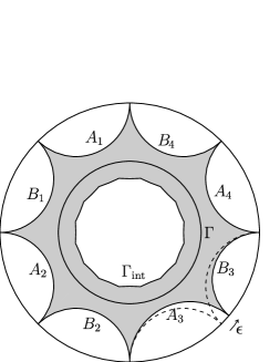
Figure 6: The shadowed region is one of the domains considered in Section 4.2

By Theorem 4.9, there exists a minimal graph $u:\Omega\to{\mathbb{R}}$ which takes boundary values $+\infty$ on the $A_{i}$ edges, $-\infty$ on the $B_{i}$ edges, and $0$ on the $C_{i}$ edges. Let $\Gamma\subset\Omega$ be a curve homologous to $\Gamma_{\rm int}$. Hence,

$$F_{u}(\Gamma)=\sum_{i}F_{u}(A_{i,n})+\sum_{i}F_{u}(B_{i,n})+\sum_{i}F_{u}(\Gamma_{i,n})$$

$$=\alpha_{n}-\beta_{n}+\sum_{i}F_{u}(\Gamma_{i,n}),$$

where $\alpha_{n}=\sum_{i}|A_{i,n}|$ and $\beta_{n}=\sum_{i}|B_{i,n}|$. Since $\alpha_{n}-\beta_{n}$ does not depend on $n$, we obtain

$$|F_{u}(\Gamma)-\alpha_{1}+\beta_{1}|\leq\sum_{i}|F_{u}(\Gamma_{i,n})|\leq\sum_{i}|\Gamma_{i,n}|.$$

Finally, we know that $\sum_{i}|\Gamma_{i,n}|\to 0$, so $F_{u}(\Gamma)=\alpha_{1}-\beta_{1}>0$.

4.3 The uniqueness problem in ${\mathbb{H}}^{2}\times{\mathbb{R}}$

In this section we study the uniqueness of solutions constructed in Theorems 4.9 and 4.12. In the first subsection, we give a maximum principle for solutions of the Dirichlet problem under some constraints. In the second, we construct a counterexample to a general uniqueness result.

4.3.1 Maximum principle

Maximum principles for unbounded domains in ${\mathbb{H}}^{2}$ are already known in special cases. For example, the proof of Collin and Rosenberg for the maximum principle in [3] admits the following generalization.

Theorem 4.13 ([3]).

Let $\Omega\subset{\mathbb{H}}^{2}$ be a domain (not necessarily simply connected) whose boundary is composed of a finite number of convex arcs together with their endpoints, possibly at infinity. Assume the following condition (C-R) holds. Consider a domain ${\cal O}\subset\Omega$ and two minimal graphs $u_{1},u_{2}$ on ${\cal O}$ which extend continuously to $\overline{\cal O}$. If $u_{1}\leq u_{2}$ on $\partial{\cal O}$, then $u_{1}\leq u_{2}$ in ${\cal O}$.

The aim of this section is to prove that we can weaken the hypothesis on the asymptotic behaviour of $\Omega$ when some constraints are satisfied by the boundary data. Before stating our result, we need to introduce some definitions. We notice that some notations for domains we consider are different from the ones in Subsection 4.1.3.

We consider domains $\Omega\subset{\mathbb{H}}^{2}$ whose boundary $\partial_{\infty}\Omega$ is composed of a finite number of open arcs $C_{i}$ in ${\mathbb{H}}^{2}$ and arcs $D_{i}$ in $\partial_{\infty}{\mathbb{H}}^{2}$ together with their endpoints (the $C_{i}$ are not supposed to be convex). The endpoints of the arcs $C_{i}$ and $D_{i}$ are called vertices of $\Omega$ and those in $\partial_{\infty}{\mathbb{H}}^{2}$ are called ideal vertices of $\Omega$. Let $p$ be an ideal vertex of $\Omega$ and $\Gamma_{1}$ and $\Gamma_{2}$ be two adjacent boundary arcs at $p$. Let $(\phi,\theta)$ be polar coordinates centered at $p$. Consider a parametrization of $\Gamma_{i}$, $\gamma_{i}:[0,1]\rightarrow\overline{\{\phi\leq 0\}}^{\infty}$, with $\gamma_{i}(0)=p$ and $\gamma_{i}(1)\in\{\phi=0\}$. We denote the polar coordinates of the parametrization by $\gamma_{i}(t)=(\phi_{i}(t),\theta_{i}(t))$ and assume that $\theta_{1}(1)\leq\theta_{2}(1)$.

Definition 4.14.

We say that $\Omega$ has necks near $p$ if

$$\liminf_{\begin{subarray}{c}q\in\Gamma_{1}\\ q\rightarrow p\end{subarray}}d(q,\Gamma_{2})=\liminf_{\begin{subarray}{c}q\in\Gamma_{2}\\ q\rightarrow p\end{subarray}}d(q,\Gamma_{1})=0$$

and the domain $\Omega$ is called admissible if, for every ideal vertex $p$ of $\Omega$, we have one of the following situations:

• $\Omega$ has necks near $p$ or

• $\displaystyle\liminf_{t\rightarrow 0}\theta_{2}(t)>0$ and $\displaystyle\limsup_{t\rightarrow 0}\theta_{1}(t)<\pi$.

The limits of the second type do not depend on the choice of polar coordinates. We notice that, if all $C_{i}$ are convex arcs (as in section 4.1.3), every ideal vertex is of second type i.e. $\Omega$ is admissible. The hypothesis type $2$ means that the adjacent arcs do not arrives “tangentially” to $\partial_{\infty}{\mathbb{H}}^{2}$ on the same side of $p$. As in Figure 7, consider an ideal vertex $p$ such that, near $p$, $\Omega$ is the domain between to horocycles $p$. The distance between $\Gamma_{1}$ and $\Gamma_{2}$ is constant so $p$ is not a type 1 vertex. Besides we have $\lim_{t\rightarrow 0}\theta_{2}(t)=0$, thus $p$ is not a type 2 vertex. This is the kind of situation that we avoid by our definition.

Figure 7: An ideal vertex which is neither type 1 nor type 2

Let $p$ be an ideal vertex of an admissible domain $\Omega$. A priori, this point is the endpoint of $2n$ arcs $\Gamma_{i}$ in $\partial_{\infty}\Omega$ (see Figure 8). As above, let $\gamma_{i}:[0,1]\rightarrow\overline{\{\phi\leq 0\}}^{\infty}\subset{\mathbb{H}}^{2}\cup\partial_{\infty}{\mathbb{H}}^{2}$, $\gamma_{i}(t)=(\phi_{i}(t),\theta_{i}(t))$, be a parametrization of $\Gamma_{i}$, with $\gamma_{i}(0)=p$ and $\gamma_{i}(1)\in\{\phi=0\}$. We assume that $\theta_{i}(1)<\theta_{j}(1)$ if $i<j$. Thus $\Omega\cap\{\phi\leq 0\}$ is included in the $n$ connected components of $\{\phi\leq 0\}\backslash(\cup_{i}\Gamma_{i})$ between $\Gamma_{2k-1}$ and $\Gamma_{2k}$, for $k=1,\cdots,n$. When $u$ is a minimal graph on $\Omega$ the study of $u$ on the part between $\Gamma_{2k-1}$ and $\Gamma_{2k}$ depends only on the values of $u$ on $\Gamma_{2k-1}$, $\Gamma_{2k}$ and the other boundary arcs of $\Omega\cap\{\phi\leq 0\}$ between $\Gamma_{2k-1}$ and $\Gamma_{2k+1}$. Thus the study on each part will be done separately; so we can assume that each ideal vertex is the endpoint of only two arcs in $\partial_{\infty}\Omega$.

Figure 8: An ideal vertex with more than two adjacent boundary arcs

Let $u$ be a minimal graph on an admissible domain $\Omega$. We say that $u$ is admissible or an admissible solution if

• $u$ extends continuously to $\cup_{i}D_{i}$,

• $u$ tends to $+\infty$ on $A(u)\subset\partial\Omega$ with $A(u)$ is a finite union of open subarcs of $\cup_{i}C_{i}$,

• $u$ tends to $-\infty$ on $B(u)\subset\partial\Omega$ with $B(u)$ is a finite union of open subarcs of $\cup_{i}C_{i}$ and

• $u$ extends continuously to $\cup_{i}C_{i}\backslash\overline{A(u)\cup B(u)}$.

We remark that each connected component of $A(u)$ and $B(u)$ is a geodesic arc (see Theorem 10.4 in [12] for the Euclidean case and Lemma 2.3). Also, we do not say anything about the values of $u$ at the vertices of $\Omega$ and the endpoints of $A(u)$ and $B(u)$. Thus, in the following, the hypotheses on the boundary values of an admissible solution $u$ will be only made where it is well defined i.e. $\cup_{i}D_{i}$, $A(u)$, $B(u)$ and $\cup_{i}C_{i}\backslash\overline{A(u)\cup B(u)}$. As an example, in Theorem 4.15, we shall write $u_{2}\leq u_{1}$ on $\partial_{\infty}\Omega$, this means that, $A(u_{2})\subset A(u_{1})$, $B(u_{1})\subset B(u_{2})$ and $(\cup_{i}D_{i})\bigcup(\cup_{i}C_{i}\backslash\overline{A(u_{2})\cup B(u_{1})}$ is non empty and $u_{2}\leq u_{1}$ on it (on $A(u_{1})\backslash\overline{A(u_{2})}$ and $B(u_{2})\backslash\overline{B(u_{1})}$ the inequality is automatically satisfied). When $(\cup_{i}D_{i})\bigcup(\cup_{i}C_{i}\backslash\overline{A(u_{2})\cup B(u_{1})}$ is empty then $u_{1}$ and $u_{2}$ are solutions of the Dirichlet problem studied in Theorem 4.12 and we already know that $u_{1}-u_{2}$ is constant so no new theorem is needed. Let us now state our generalization of Theorem 4.13.

Theorem 4.15 (General maximum principle).

Let $\Omega\subset{\mathbb{H}}^{2}$ be an admissible domain and $u_{1}$ and $u_{2}$ be two admissible solutions. We assume that $u_{2}\leq u_{1}$ on $\partial_{\infty}\Omega$. Also we assume that the behaviour near each ideal vertex $p\in\partial_{\infty}{\mathbb{H}}^{2}$ is one of the following:

• $\Omega$ has necks near $p$,

• $\liminf_{p}u_{1}+\varepsilon>\limsup_{p}u_{2}$ (for every $\varepsilon>0$) along both boundary components with $p$ as endpoint,

• if $A\subset A(u_{2})\subset A(u_{1})$ (resp. $B\subset B(u_{1})\subset B(u_{2})$) is a geodesic arc with $p$ as endpoint and $\Gamma$ is the other boundary arc in $\partial_{\infty}\Omega$ with endpoint $p$, $\liminf_{p}u_{1}+\varepsilon>\limsup_{p}u_{2}$ (for every $\varepsilon>0$) along $\Gamma$.

Then we have $u_{2}\leq u_{1}$ in $\Omega$.

Let us make some comments on the hypotheses of the theorem. First the hypothesis (C-R) made by Collin and Rosenberg in Theorem 4.13 implies that, near each ideal vertex, $\Omega$ has necks. Thus Theorem 4.15 generalizes Theorem 4.13. We notice that, when a vertex $p$ is the endpoint of two geodesic arcs (for example, one in $A(u_{2})$ and the other in $B(u_{1})$), $\Omega$ has necks near $p$. Moreover, the hypothesis $\liminf_{p}u_{1}+\varepsilon>\limsup_{p}u_{2}$ along a boundary component which has $p$ as endpoint means that we are in one of the following three cases:

$$\liminf_{p}u_{1}=+\infty\textrm{ and }\limsup_{p}u_{2}<+\infty,$$ (6)

$$\liminf_{p}u_{1}>-\infty\textrm{ and }\limsup_{p}u_{2}=-\infty,$$ (7)

$$-\infty<\limsup_{p}u_{2}\leq\liminf_{p}u_{1}<+\infty.$$ (8)

in the third case, the boundary data for $u_{1}$ and $u_{2}$ “stay close” so it is the more complicated case. Hence the proof will be written in this case; small changes suffice to treat the first two cases. We remark that our theorem does not deal with the case $\lim_{p}u_{1}=\lim_{p}u_{2}=+\infty$.

The proof of Theorem 4.15 is long and needs some preliminary results that may have their own interest.

Let $\Omega$ be a domain in ${\mathbb{H}}^{2}$, we say that $\Omega$ has a finite number of point-ends if there exist $p_{1},\cdots,p_{n}\in\partial_{\infty}{\mathbb{H}}^{2}$ and $(\phi_{i},\theta_{i})$ polar coordinates centered at $p_{i}$ such that:

$$\textrm{for every }m<0\textrm{ and }i,\ \Omega\cap\cup_{i}\{\phi_{i}>m\}\textrm{ is compact and }\Omega\cap\{\phi_{i}<m\}\neq\emptyset.$$

The $p_{i}$ are the point-ends (we do not assume anything about the connectedness of $\Omega\cap\{\phi_{i}<m\}$). We say the point-end $p_{i}$ is in a corridor if there exists $\alpha\in(0,\pi/2)$ and $m<0$ such that:

$$\Omega\cap\{\phi_{i}<m\}\subset\{\alpha<\theta_{i}<\pi-\alpha\}$$

We notice that these definitions do not depend on the choice of $(\phi_{i},\theta_{i})$.

Let $\Omega\subset{\mathbb{H}}^{2}$ be an admissible domain and $u_{1}$ and $u_{2}$ be two admissible solutions on $\Omega$. We assume that $u_{1}\geq u_{2}$ on $\partial_{\infty}\Omega$. Let $\varepsilon$ be positive with $O=\{u_{1}\leq u_{2}-\varepsilon\}$ nonempty. Since $u_{1}\geq u_{2}$ on the $D_{i}$, $O$ has a finite number of point-ends that are among the ideal vertices of $\Omega$. With this setting, we have a first result which follows the ideas of Collin and Krust in [2].

Proposition 4.16.

Let $\Omega\subset{\mathbb{H}}^{2}$, $u_{1}$, $u_{2}$ admissible solutions on $\Omega$, $\varepsilon>0$ and $O$ be as above. The subset $O$ is assumed to be nonempty and, for each point-end $p$, we assume that either $p$ is in a corridor or $\Omega$ has necks near $p$. Then the function $u_{1}-u_{2}$ is not bounded below.

First, we can assume that $\varepsilon$ is a regular value of $u_{2}-u_{1}$ and so $\partial O\cap\Omega$ is smooth. Let us assume that the proposition is not satisfied i.e. there exists $M>0$ such that $u_{2}-u_{1}\leq M$.

Let $K$ be a domain in ${\mathbb{H}}^{2}$ with smooth boundary such that $\overline{\Omega\cap K}$ is compact. We notice that $\partial O\cap(\cup_{i}D_{i})=\emptyset$ and $\partial O\cap(\cup_{i}C_{i})\subset\overline{A(u_{2})\cup B(u_{1})}$. For $\delta>0$ small, we denote by $N_{\delta}$ the closed $\delta$-neighborhood of $\overline{A(u_{2})\cup B(u_{1})}$ and define:

$$O(K,\delta)=\big{(}O\cap K\big{)}\backslash N_{\delta}$$

We notice that $\partial O(K,\delta)$ is piecewise smooth and is included in $\Omega$. This boundary can be decomposed in three parts:

• $\partial_{1}(K,\delta)=\partial O(K,\delta)\cap\partial O$ on which $u_{2}-u_{1}=\varepsilon$,

• $\partial_{2}(K,\delta)=\partial O(K,\delta)\cap\partial N_{\delta}$,

• $\partial_{3}(K,\delta)=\partial O(K,\delta)\cap(\partial K\backslash\partial O)$.

Figure 9: The boundary parts of $O(K,\delta)$

Let us define $u=u_{2}-u_{1}-\varepsilon$, $X=X_{u_{2}}-X_{u_{1}}$ and $\nu$ the outgoing normal from $O(K,\delta)$. Let us prove that:

$$\lim_{\delta\rightarrow 0}\left|\int_{\partial_{2}(K,\delta)}u\langle X,\nu\rangle\right|=0$$ (9)

Since $\displaystyle\left|\int_{\partial_{2}(K,\delta)}u\langle X,\nu\rangle\right|\leq M\int_{\partial_{2}(K,\delta)}\left|\langle X,\nu\rangle\right|$, it suffices to prove

Claim 4.17.

we have:

$$\lim_{\delta\rightarrow 0}\int_{\partial_{2}(K,\delta)}\left|\langle X,\nu\rangle\right|=0$$

The connected components of $A(u_{2})\cup B(u_{1})$ are geodesic arcs. In such a component, for $\beta>0$, a subarc is composed of points at a distance larger than $\beta$ from the endpoints. We denote by $I(\beta)$ the union of all these subarcs. Now, in $\partial N_{\delta}$, some points are at distance $\delta$ from $I(\beta)$ (we denote this part $J_{1}(\delta,\beta)$) and the other points are at distance $\delta$ from $\overline{A(u_{2})\cup B(u_{1})}\backslash I(\beta)$ (we denote this part $J_{2}(\delta,\beta)$). We notice that the length of $J_{2}(\delta,\beta)$ is bounded and

$$\lim_{\delta\rightarrow 0}{\ell}(J_{2}(\delta,\beta))=2n_{0}\beta$$

where $n_{0}$ is the number of endpoints of $A(u_{2})\cup B(u_{1})$ in ${\mathbb{H}}^{2}$. We have:

$$\int_{\partial_{2}(K,\delta)}\left|\langle X,\nu\rangle\right| =\int_{J_{1}(\delta,\beta)\cap\partial O(K,\delta)}\left|\langle X,\nu\rangle\right|+\int_{J_{2}(\delta,\beta)\cap\partial O(K,\delta)}\left|\langle X,\nu\rangle\right|$$

$$\leq\int_{J_{1}(\delta,\beta)\cap\partial O(K,\delta)}|X|+2\ell(J_{2}(\delta,\beta))$$

$$\leq\ell(J_{1}(\delta,\beta)\cap\partial O(K,\delta))\max_{J_{1}(\delta,\beta)\cap\partial O(K,\delta)}|X|+2\ell(J_{2}(\delta,\beta))$$

As $\delta$ goes to $0$, $\max_{J_{1}(\delta,\beta)\cap\partial O(K,\delta)}|X|$ tends to $0$ and $\ell(J_{1}(\delta,\beta)\cap\partial O(K,\delta))$ is bounded (since $\Omega\cap K$ is compact). Hence for every small $\mu>0$, we can take $\beta$ and $\delta$ small enough such that:

$$\int_{\partial_{2}(K,\delta)}\left|\langle X,\nu\rangle\right|\leq\mu$$

Claim 4.17 is proved.

Also we have (see Lemma 1 in [2] for the first inequality).

$$\iint_{O(K,\delta)}|X|^{2}\leq\int_{\partial O(K,\delta)}u\langle X,\nu\rangle =\int_{\partial_{1}(K,\delta)}u\langle X,\nu\rangle+\int_{\partial_{2}(K,\delta)}u\langle X,\nu\rangle+\int_{\partial_{3}(K,\delta)}u\langle X,\nu\rangle$$

$$=\int_{\partial_{2}(K,\delta)}u\langle X,\nu\rangle+\int_{\partial_{3}(K,\delta)}u\langle X,\nu\rangle$$

We notice that $|X|^{2}\geq 0$ and $\int_{\partial_{3}(K,\delta)}u|\langle X,\nu\rangle|\leq 2M\ell(\partial_{3}(K,\delta))\leq 2M\ell(\partial_{3}(K,0))$. By (9), taking $\delta\rightarrow 0$ in the above inequality, we get

$$\iint_{O(K,0)}|X|^{2}\leq\int_{\partial_{3}(K,0)}u\langle X,\nu\rangle$$ (10)

Let $p_{1},\cdots,p_{n}$ be the point-ends of $O$; they are numbered such that $p_{1},\cdots,p_{k}$ are in a corridor and $\Omega$ has necks near $p_{k+1},\cdots,p_{n}$. For each $i$ we consider polar coordinates $(\phi_{i},\theta_{i})$ centered at $p_{i}$, chosen such that the hyperbolic half-planes $\{\phi_{i}<0\}$ do not intersect. Let $\alpha>0$ be such that, for every $i\in\{1,\cdots,k\}$, $O\cap\{\phi_{i}<0\}\subset\{\alpha\geq\theta_{i}\geq\pi-\alpha\}$ with $\alpha>0$.

Let $\phi$ and $\psi$ be negative and $\mu>0$. Since $\Omega$ has necks near each $p_{i}$ with $i\geq k+1$, there is in $\Omega\cap\{\phi_{i}<\psi\}$ a geodesic $\Gamma_{i}$ of length less than $\mu$ joining the two adjacent arcs at $p_{i}$. Let $K$ be the compact part of $\Omega$ delimited by the geodesic $\{\phi_{i}=\phi\}$ for $i\leq k$ and the geodesic $\Gamma_{i}$ for $i\geq k+1$. Besides we denote

$$O_{\phi,\psi}=O\backslash\left(\Big{(}\bigcup_{i=1}^{k}\{\phi_{i}<\phi\}\Big{)}\bigcup\Big{(}\bigcup_{i=k+1}^{n}\ \{\phi_{i}<\psi\}\Big{)}\right)$$

From (10), we obtain:

$$\iint_{O_{\phi,\psi}}|X|^{2}\leq\iint_{O(K,0)}|X|^{2} \leq\int_{\partial_{3}(K,0)}u\langle X,\nu\rangle$$

$$\leq\sum_{i=1}^{k}\int_{O\cap\{\phi_{i}=\phi\}}u\langle X,\nu\rangle+\sum_{i=k+1}^{n}\int_{O\cap\Gamma_{i}}u\langle X,\nu\rangle$$

$$\leq M\sum_{i=1}^{k}\int_{O\cap\{\phi_{i}=\phi\}}|X|+2M(n-k)\mu$$

Thus letting $\mu$ going to $0$, $\psi$ going to $-\infty$ and denoting by $O_{\phi}$ the subset $O_{\phi,-\infty}$ and $I_{\phi}=\bigcup_{i=1}^{k}O\cap\{\phi_{i}=\phi\}$ a part of the boundary, we get

$$\iint_{O_{\phi}}|X|^{2}\leq M\int_{I_{\phi}}|X|$$ (11)

Let us denote by $\eta(\phi)$ the integral in the right-hand term. By Schwartz’s Lemma, we obtain:

$$\eta^{2}(\phi)\leq\ell(I_{\phi})\int_{I_{\phi}}|X|^{2}\leq C(\alpha)\int_{I_{\phi}}|X|^{2}$$

where $C(\alpha)=k\int_{\alpha}^{\pi-\alpha}\frac{d\theta}{\sin(\theta)}$. Thus $\int_{I_{\phi}}|X|^{2}\geq\eta^{2}(\phi)/C(\alpha)$ and, in (11), this gives:

$$\mu_{0}+\int_{\phi}^{0}\frac{\eta^{2}(t)}{C(\alpha)}dt\leq M\eta(\phi)$$ (12)

with $\mu_{0}>0$. Let $\zeta$ be the function defined on $I=(-(M^{2}C(\alpha))/\mu_{0},0]$ by :

$$\frac{M}{\mu_{0}}-\frac{1}{\zeta(t)}=-\frac{t}{MC(\alpha)}$$

This function $\zeta$ satisfies $\zeta(0)=\mu_{0}/M$ and $\zeta^{\prime}=-\zeta^{2}/(MC(\alpha))$. Thus for $\phi\in I$ we have $\zeta(\phi)\leq\eta(\phi)$. But $\eta(\phi)\leq 2\ell(I_{\phi})\leq 2C(\alpha)$ and $\lim_{t\rightarrow-(M^{2}C(\alpha))/\mu_{0}}\zeta(t)=+\infty$. We have a contradiction.

We have a first lemma that allows us to bound admissible solutions.

Lemma 4.18.

Let $\Omega$ be an admissible domain in ${\mathbb{H}}^{2}$. Let $u$ be an admissible solution with $B(u)=\emptyset$ and assume there exists $m\in{\mathbb{R}}$ such that $u\geq m$ on $\partial_{\infty}\Omega$. Then $u$ is bounded below in $\Omega$.

There are only a finite number of points where such a lower-bound is unknown: the vertices of $\Omega$ and the endpoints of arcs in $A(u)$. We notice that there are only a finite number of such points. When an endpoint of $A(u)$ or a vertex of $\Omega$ is in ${\mathbb{H}}^{2}$, a lower-bound is given by the maximum principle for bounded domains. So let us consider an ideal vertex $p$. Let $(\phi,\theta)$ be polar coordinates centered at $p$ and consider $\Omega^{\prime}=\Omega\cap\{\phi<0\}$. Let $m^{\prime}\leq m$ be such that $u\geq m^{\prime}$ on $\Omega\cap\{\phi=0\}$; let us prove that $u\geq m^{\prime}$ in $\Omega^{\prime}$.

Take $t<0$ and consider the minimal graph $w_{t}$ given by Lemma 4.1 on the domain $\{\phi>t\}$ which takes the value $-\infty$ on $\{\phi=t\}$ and $m^{\prime}$ on the other boundary arc. We know that $w_{t}\leq m^{\prime}$ on $\{\phi>t\}$. By the maximum principle for bounded domain, $w_{t}\leq u$ on $\Omega^{\prime}\cap\{\phi>t\}$. As $t\rightarrow-\infty$, $w_{t}\rightarrow m^{\prime}$; hence $m^{\prime}\leq u$ on $\Omega^{\prime}$.

In the proof of Theorem 4.15, type 2 ideal vertices are the hardest to deal with. Thus we need to be more precise for a bound near such a vertex. In the following lemma, we use the minimal graph defined in Lemma 4.1 to control a minimal graph on one side of a type 2 ideal vertex.

Lemma 4.19.

For every $0<\bar{\theta}\leq\pi/2$, there is a continuous increasing function $H_{\bar{\theta}}:[0,\bar{\theta})\rightarrow{\mathbb{R}}_{+}$ with $H_{\bar{\theta}}(0)=0$ such that the following is true.

Let $\Omega$ be an admissible domain in ${\mathbb{H}}^{2}$ and $p$ an ideal vertex of $\Omega$. We consider polar coordinates $(\phi,\theta)$ centered at $p$. For $i=1,2$, let

$$\gamma_{i}:\begin{array}[]{cl}(0,1]&\longrightarrow\overline{\{\phi\leq 0\}}^{\infty}\\ t&\longmapsto(\phi_{i}(t),\theta_{i}(t))\end{array}$$

be parametrizations of the two adjacent arcs in $\partial_{\infty}\Omega$ with $p$ as endpoint; we assume $\lim_{t\rightarrow 0}\gamma_{i}(t)=p$ $\gamma_{i}(1)\in\{\phi=0\}$ and $\theta_{1}(1)<\theta_{2}(1)$. Let $\bar{\theta_{2}}=\liminf_{t\rightarrow 0}\theta_{2}(t)$; we assume $\bar{\theta_{2}}>0$.

Let $u$ be an admissible solution on $\Omega$ such that $u\geq m$ in $\gamma_{1}((0,1])$. Then for every $\theta_{0}$ and $\bar{\theta}$ with $0<\theta_{0}<\bar{\theta}<\bar{\theta_{2}}$, there exists $\phi_{0}<0$ such that :

$$u\geq m-H_{\bar{\theta}}(\theta_{0})\textrm{ on }\Omega\cap\{\phi<\phi_{0},\theta<\theta_{0}\}$$

Let us consider $(\phi,\theta)$ polar coordinates at a point in $\partial_{\infty}{\mathbb{H}}^{2}$ and $\bar{\theta}\in(0,\pi/2]$. On $\Omega_{\bar{\theta}}=\{(\theta,\phi)\in{\mathbb{H}}^{2}|\theta<\bar{\theta}\}$, we consider the minimal graph $h_{\bar{\theta}}(\phi,\theta)=h_{\bar{\theta}}(\theta)$ given by Lemma 4.1 with $h_{\bar{\theta}}=0$ on $\{\theta=0\}$ and $\dfrac{\partial h_{\bar{\theta}}}{\partial\nu}=+\infty$ along $\{\theta=\bar{\theta}\}$, where $\nu$ is the outward pointing normal vector. For $\theta_{0}<\bar{\theta}$, we define:

$$H_{\bar{\theta}}(\theta_{0})=h_{\bar{\theta}}(\theta_{0}+\frac{\theta_{0}}{\bar{\theta}}(\bar{\theta}-\theta_{0}))=\max_{\{0 \leq\theta\leq\theta_{0}+\frac{\theta_{0}}{\bar{\theta}}(\bar{\theta}-\theta_{0})\}}h_{\bar{\theta}}$$

We remark that $\theta_{0}<\theta_{0}+\frac{\theta_{0}}{\bar{\theta}}(\bar{\theta}-\theta_{0})<\bar{\theta}$ when $0<\theta_{0}<\bar{\theta}$. $H_{\bar{\theta}}$ is a continuous increasing function with $H_{\bar{\theta}}(0)=0$.

Figure 10: $O_{s}$ is the shadowed domain

Let $\Omega$, $u$, $(\phi,\theta)$ be as in the lemma. Let $\bar{\theta}$ be less than $\bar{\theta_{2}}$; by changing $\phi$, we can assume that $\theta_{2}(t)\geq\bar{\theta}$ for $t\in(0,1]$. Let $s$ be negative, we consider the geodesic $B_{s}$ joining the points with polar coordinates $(s,0)$ and $(0,0)$ and the arc $D_{s}$ in $\partial_{\infty}{\mathbb{H}}^{2}\cap\{\phi\leq 0\}$ joining both points. Let $C_{s}$ be the equidistant to $B_{s}$ which is at distance $d_{\bar{\theta}}$ (see (2)) and is in the half-plane delimited by $B_{s}$ and $D_{s}$ (see Figure 10). We denote by $O_{s}$ the domain bounded by $C_{s}$ and $D_{s}$ ($O_{s}$ is included in $\theta\leq\bar{\theta}$). On $O_{s}$, we consider $k_{s}$ the minimal graph given by Lemma 4.1 with $k_{s}=0$ on $D_{s}$ and $\dfrac{\partial k_{s}}{\partial\nu}=+\infty$ on $C_{s}$. We notice that $k_{s}>0$ on $O_{s}$. Since $\bar{\theta}<\theta_{2}(t)$ for every $t$, the boundary of $O_{s}\cap\Omega$ is composed of subarcs of $C_{s}$ and subarcs of $\gamma_{1}$. Hence, by the maximum principle for bounded domains, $u\geq m-k_{s}$ on $\Omega\cap O_{s}$. Let $s$ go to $-\infty$, $k_{s}$ converges to the solution $k_{-\infty}$ on $O_{-\infty}$ with $h_{-\infty}=0$ on $D_{-\infty}$ and $\dfrac{\partial h_{-\infty}}{\partial\nu}=+\infty$ on $C_{-\infty}$ given by Lemma 4.1. Moreover, we have $m-k_{-\infty}\leq u$ on $\Omega\cap O_{-\infty}$. Fix $0<\theta_{0}<\bar{\theta}$. Because of the definition of $H_{\bar{\theta}}$, there is $\phi_{0}$ such that

$$k_{-\infty}\leq H_{\bar{\theta}}(\theta_{0})\textrm{ on }\{\phi<\phi_{0},\theta<\theta_{0}\}$$

which concludes the lemma.

Actually, this Lemma says that if a solution is bounded below on one of the two boundary components with $p$ as endpoint, then the solution is bounded below in some “sectorial” neighborhood of this boundary component.

Now we have the following result

Proposition 4.20.

Let $\Omega$ be an admissible domain and $u$ an admissible solution. Let $p\in\partial\Omega$ be a type 2 ideal vertex of $\Omega$. We assume there exists $m\in{\mathbb{R}}$ such that $u\geq m$ near $p$ on $\partial\Omega$. Then, for every $\varepsilon>0$, $u\geq m-\varepsilon$ in a neighborhood of $p$ in $\Omega$.

Let $(\phi,\theta)$ be polar coordinates centered at $p$. We assume that $u\geq m$ on $\partial\Omega\cap\{\phi\leq 0\}$. Let $h$ be the minimal graph over $\{\phi<0\}$ given by Lemma 4.1 with boundary values $h=-\infty$ on $\{\phi=0\}$ and $h=m$ on the other boundary arc . For every $\varepsilon>0$, we have $h\geq m-\varepsilon$ on a neighborhood of $p$, so it suffices to prove that $h\leq u$ on $\Omega\cap\{\phi<0\}$.

If $\{u<h\}$ is nonempty, consider $\varepsilon>0$ a regular value of $h-u$ such that $\{u<h-\varepsilon\}\neq\emptyset$. The only possible point-end of $\{u<h-\varepsilon\}$ is $p$. Let us prove that $p$ is in a corridor. Let $\gamma_{i}=(\phi_{i},\theta_{i})$ be parametrizations defined on $(0,1]$ of both boundary arcs adjacent at $p$ in $\overline{\{\phi<0\}}^{\infty}$ with $\lim_{t\rightarrow 0}\gamma_{i}(t)=p$, $\phi_{1}(1)=\phi_{2}(1)=0$ and $\theta_{1}(1)<\theta_{2}(1)$. Since $p$ is of type 2, $\liminf_{t\rightarrow 0}\theta_{2}(t)>0$. Let $0<\bar{\theta}<\liminf_{t\rightarrow 0}\theta_{2}(t)$, $H_{\bar{\theta}}$ be defined by Lemma 4.19 and $\theta^{\prime}\in(0,\bar{\theta})$ such that $H_{\bar{\theta}}(\theta^{\prime})<\varepsilon$. Lemma 4.19 gives $\phi^{\prime}<0$ such that $u\geq m-H_{\bar{\theta}}(\theta^{\prime})\geq m-\varepsilon$ on $\Omega\cap\{\phi<\phi^{\prime},\theta<\theta^{\prime}\}$. Applying Lemma 4.19 also on the other side of $p$, we obtain $\phi_{0}<0$ and $\theta_{0}>0$ such that $u\geq m-\varepsilon$ in $\{\phi<\phi_{0}\}\cap\{\sin(\theta)<\sin(\theta_{0})\}$. Since $h\leq m$ in $\{\phi<0\}$, we have $\{u<h-\varepsilon\}\cap(\{\phi<\phi_{0}\}\cap\{\sin(\theta)<\sin(\theta_{0})\})=\emptyset$. Thus the end is in a corridor. Theorem 4.16 now implies that $u$ is not bounded below near $p$, that contradicts Lemma 4.18

We can now give the proof of the general maximum principle (Theorem 4.15). We recall that the proof is written in the case (8).

[Proof of Theorem 4.15] Let $\Omega$, $u_{1}$ and $u_{2}$ be as in the theorem and assume that $u_{2}\leq u_{1}$ is not true in the whole $\Omega$, so we can choose $\varepsilon>0$ such that $\{u_{1}\leq u_{2}-\varepsilon\}$ is nonempty. Since $u_{1}>u_{2}-\varepsilon$ on the arcs $D_{i}$, the point-ends of $\{u_{1}\leq u_{2}-\varepsilon\}$ are among the ideal vertices of $\Omega$. In particular, $\{u_{1}\leq u_{2}-\varepsilon\}$ has a finite number of point-ends. Let us prove that each point-end associated to a type 2 vertex of $\Omega$ is in a corridor.

Let $p$ be a point-end which is a type 2-i vertex of $\Omega$. Let $\Gamma_{1}$ and $\Gamma_{2}$ denote the two components of $\partial_{\infty}\Omega$ with $p$ as endpoint and consider polar coordinates $(\phi,\theta)$ centered at $p$. There is $\phi_{0}$ such that

$$u_{1}\geq\liminf_{\begin{subarray}{c}x\in\Gamma_{i}\\ x\rightarrow p\end{subarray}}u_{1}-\varepsilon/4\ \textrm{ and }\ u_{2}\leq\limsup_{\begin{subarray}{c}x\in\Gamma_{i}\\ x\rightarrow p\end{subarray}}u_{2}+\varepsilon/4\ \textrm{ on }\Gamma_{i}\cap\{\phi<\phi_{0}\}$$

Using Lemma 4.19 as in the proof of Lemma 4.20, there exist $\phi_{1}<\phi_{0}$ and $\theta_{1}\in(0,\pi/2)$ such that

$$u_{1} \geq\liminf_{\begin{subarray}{c}x\in\Gamma_{1}\\ x\rightarrow p\end{subarray}}u_{1}-\varepsilon/2\textrm{ on }\Omega\cap\{\phi\leq\phi_{1},\theta<\theta_{1}\}$$

$$u_{2} \leq\limsup_{\begin{subarray}{c}x\in\Gamma_{1}\\ x\rightarrow p\end{subarray}}u_{2}+\varepsilon/2\textrm{ on }\Omega\cap\{\phi\leq\phi_{1},\theta<\theta_{1}\}$$

$$u_{1} \geq\liminf_{\begin{subarray}{c}x\in\Gamma_{2}\\ x\rightarrow p\end{subarray}}u_{1}-\varepsilon/2\textrm{ on }\Omega\cap\{\phi\leq\phi_{1},\theta>\pi-\theta_{1}\}$$

$$u_{2} \leq\liminf_{\begin{subarray}{c}x\in\Gamma_{2}\\ x\rightarrow p\end{subarray}}u_{2}+\varepsilon/2\textrm{ on }\Omega\cap\{\phi\leq\phi_{1},\theta>\pi-\theta_{1}\}$$

Thus on $\Omega\cap\{\phi\leq\phi_{1},\theta<\theta_{1}\}$, we have

$$u_{1}-u_{2}\geq\liminf_{\begin{subarray}{c}x\in\Gamma_{1}\\ x\rightarrow p\end{subarray}}u_{1}-\varepsilon/2-(\limsup_{\begin{subarray}{c}x\in\Gamma_{1}\\ x\rightarrow p\end{subarray}}u_{2}+\varepsilon/2)\geq-\varepsilon$$

In $\Omega\cap\{\phi\leq\phi_{1},\theta>\pi-\theta_{1}\}$, we also have $u_{1}-u_{2}>-\varepsilon$. So $p$ is in a corridor.

In the case the point-end $p$ of $\{u_{1}\leq u_{2}-\varepsilon\}$ is a type 2-ii vertex of $\Omega$, we can choose polar coordinates $(\phi,\theta)$ centered at $p$ such that the geodesic arc $A$ is in $\{\theta=\pi/2\}$ and $\Gamma\subset\overline{\{\theta<\pi/2\}}^{\infty}$. As above, we prove that there exist $\phi_{1}$ and $\theta_{1}>0$ such that $u_{1}-u_{2}>-\varepsilon$ in $\Omega\cap\{\phi\leq\phi_{1},\theta<\theta_{1}\}$. So, $p$ is in a corridor.

Therefore, we have proved that either the point-ends of $\{u_{1}\leq u_{2}-\varepsilon\}$ are in corridors or $\Omega$ has necks near them. Thus Proposition 4.16 assures $u_{1}-u_{2}$ is not bounded below.

Let $p$ be an ideal vertex of $\Omega$ of type 2-i. By Lemma 4.18, there are $m_{1}$ and $m_{2}$ in ${\mathbb{R}}$ such that $u_{1}\geq m_{1}$ and $u_{2}\leq m_{2}$ in a neighborhood of $p$ , so $u_{1}-u_{2}\geq m_{1}-m_{2}$ in a neighborhood of $p$. Since the number of type 2-i vertices is finite, there is $m<0$ such that $u_{1}-u_{2}\geq m$ in neighborhood of type 2-i vertices. Moreover $m$ can be chosen to be a regular value for $u_{1}-u_{2}$. So let us denote the nonempty set

$$O=\{u_{1}-u_{2}\leq m\}.$$

In fact the value of $m$ is not already fixed : in the following, we shall need to decrease $m$ a finite number of times (these changes are only linked to the geometry of the domain).

We notice that $\partial O\cap(\cup_{i}D_{i})=\emptyset$ and $\partial O\cap(\cup_{i}C_{i})\subset\overline{B(u_{1})\cup A(u_{2})}$. $O$ has a finite number of point-ends which correspond to ideal vertices of type 1 or 2-ii. Let us them denote by $p_{1},\cdots,p_{n}$ and by $(\phi_{i},\theta_{i})$ polar coordinates centered at $p_{i}$. As in the proof of Proposition 4.16, for $\delta>0$ small, we denote by $N_{\delta}$ the closed $\delta$-neighborhood of $\overline{B(u_{1})\cup A(u_{2})}$ and we define:

$$O(\phi,\delta)=O\backslash\big{(}N_{\delta}\bigcup(\cup_{i}\{\phi_{i}\leq\phi\})\big{)}$$

Its boundary $\partial O(\phi,\delta)\subset\Omega$ is piecewise smooth and is composed of three parts:

• $\partial_{1}(\phi,\delta)=\partial O(\phi,\delta)\cap\partial O$, where $u_{2}-u_{1}=-m$,

• $\partial_{2}(\phi,\delta)=\partial O(\phi,\delta)\cap\partial N_{\delta}$,

• $\partial_{3}(\phi,\delta)=\partial O(\phi,\delta)\cap(\cup_{i}\{\phi_{i}=\phi\}\backslash\partial O)$.

We call $X=X_{u_{2}}-X_{u_{1}}$ and $\nu$ the outgoing normal to $\partial O(\phi,\delta)$. We have:

$$0=\int_{\partial O(\phi,\delta)}\langle X,\nu\rangle=\int_{\partial_{1}(\phi,\delta)}\langle X,\nu\rangle+\int_{\partial_{2}(\phi,\delta)}\langle X,\nu\rangle+\int_{\partial_{3}(\phi,\delta)}\langle X,\nu\rangle$$

We notice that along $\partial_{1}(\phi,\delta)$, $\nabla u_{2}-\nabla u_{1}$ points into $O$ so $X$ points to $O$. Hence $\langle X,\nu\rangle$ is negative on $\partial_{1}(\phi,\delta)$ (see Lemma 2 in [2]). Besides, we have $|X|\leq 2$ and the length of $\partial_{3}(\phi,\delta)$ is uniformly bounded for fixed $\phi$ since either the point-ends of $O$ are in corridors or $\Omega$ has necks at them. Thus, with $K=\cap_{i}\{\phi_{i}>\phi\}$, Claim 4.17 implies that, letting $\delta$ goes to $0$, we obtain:

$$0=\int_{\partial_{1}(\phi,0)}\langle X,\nu\rangle+\int_{\partial_{3}(\phi,0)}\langle X,\nu\rangle$$

Or

$$0<-\int_{\partial_{1}(\phi,0)}\langle X,\nu\rangle=\int_{\partial_{3}(\phi,0)}\langle X,\nu\rangle$$

We can decomposed $\partial_{3}(\phi,0)$ in a finite number of parts $\gamma_{1}(\phi),\cdots,\gamma_{n}(\phi)$: $\gamma_{i}(\phi)$ is the part of $\partial_{3}(\phi,0)$ in $\{\phi_{i}=\phi\}$. Thus we have:

$$-\int_{\partial_{1}(\phi,0)}\langle X,\nu\rangle=\sum_{i=1}^{n}\int_{\gamma_{i}(\phi)}\langle X,\nu\rangle$$

The left-hand term is positive and increases as $\phi\searrow-\infty$. Thus we get a contradiction and Theorem 4.15 is proved once we have established the following claim:

Claim 4.21.

For every $i$, we have

$$\limsup_{\phi\rightarrow-\infty}\int_{\gamma_{i}(\phi)}\langle X,\nu\rangle\leq 0$$

First we suppose $p_{i}$ is a type 1 vertex. Let $\phi_{0}<0$ be fixed. Since $p_{i}$ is a type 1 vertex, for each $\mu>0$ there is a geodesic arc $\Gamma\subset\Omega\cap\{\phi<\phi_{0}\}$ of length less than $\mu$. $\Gamma$ separates $\Omega\cap\{\phi<\phi_{0}\}$ into a non compact component and a compact part $\Omega_{\Gamma}$. Let $\phi_{1}<\phi_{0}$ be such that $\Gamma\in\{\phi>\phi_{1}\}$. As above we can compute the flux of $X$ along the boundary of $O\cap\Omega_{\Gamma}$ and we get:

$$0=\int_{\partial(O\cap\Omega_{\Gamma})}\langle X,\nu^{\prime}\rangle=\int_{\partial_{1}(\phi_{1},0)\cap\Omega_{\Gamma}}\langle X,\nu^{\prime}\rangle+\int_{O\cap\Gamma}\langle X,\nu^{\prime}\rangle-\int_{\gamma_{i}(\phi_{0})}\langle X,\nu\rangle$$

with $\nu^{\prime}$ the outgoing normal from $O\cap\Omega_{\Gamma}$. The sign of the last term comes from the fact that $\nu^{\prime}=-\nu$ along $\gamma_{i}(\phi)$. As above, $X$ points to $O\cap\Omega_{\Gamma}$ along $\partial_{1}(\phi_{1},0)\cap\Omega_{\Gamma}$, thus $\int_{\partial_{1}(\phi_{1},0)\cap\Omega_{\Gamma}}\langle X,\nu^{\prime}\rangle\leq 0$ and

$$\int_{\gamma_{i}(\phi_{0})}\langle X,\nu\rangle=\int_{\partial_{1}(\phi_{1},0)\cap\Omega_{\Gamma}}\langle X,\nu^{\prime}\rangle+\int_{O\cap\Gamma}\langle X,\nu^{\prime}\rangle\leq 2\ell(\Gamma)\leq 2\mu$$

The above inequality occurs for every $\mu>0$. Then $\int_{\gamma_{i}(\phi_{0})}\langle X,\nu\rangle\leq 0$ and the claim is proved when $p_{i}$ is a type $1$ vertex of $\Omega$.

Let us now suppose $p_{i}$ is a type 2-ii vertex of $\Omega$. We choose the polar coordinates centered $p_{i}$ such that the geodesic arc $A$ is in $\{\theta=\pi/2\}$ and the arc $\Gamma$ is in $\{\theta<\pi/2\}$. We fix $\phi_{0}<0$. Let $G:[0,1]\rightarrow{\mathbb{H}}^{2}\cup\partial_{\infty}{\mathbb{H}}^{2}$ be a parametrization of $\Gamma$, in polar coordinates $G(t)=(\phi(t),\theta(t))$ for $t>0$ with $\phi(1)=\phi_{0}$. Since $p_{i}$ is an endpoint of $\Gamma$, $\lim_{t\rightarrow 0}\phi(t)=-\infty$. Let $\theta_{\infty}$ be $\limsup_{t\rightarrow 0}\theta(t)$. If $\theta_{\infty}=\pi/2$, we have $\liminf_{t\rightarrow 0}d(G(t),A)=0$ as in type 1 vertices and we can apply the above proof.

We then assume $\theta_{\infty}<\pi/2$. Let us consider $\bar{\theta}\in(\theta_{\infty},\pi/2)$. By changing $\phi_{0}$, we can assume that $\theta(t)<\bar{\theta}$ for every $t\in(0,1]$.

Let us define $u_{1}^{\infty}=\liminf_{\begin{subarray}{c}x\in\Gamma\\ x\rightarrow p\end{subarray}}u_{1}(x)$ and $u_{2}^{\infty}=\limsup_{\begin{subarray}{c}x\in\Gamma\\ x\rightarrow p\end{subarray}}u_{2}(x)$. From Lemma 4.19 and Proposition 4.20, there are $\bar{\phi}<\phi_{0}$ and $\overline{m}\geq 1$ such that $u_{1}\geq u_{1}^{\infty}-1$ on $\Omega\cap\{\phi<\bar{\phi}\}$ and $u_{2}\leq u_{2}^{\infty}+\overline{m}$ on $\Omega\cap\{\phi<\bar{\phi},\theta<\bar{\theta}\}$. Thus on $\Omega\cap\{\phi<\bar{\phi},\theta\leq\bar{\theta}\}$, $u_{1}-u_{2}\geq u_{1}^{\infty}-1-u_{2}^{\infty}-\bar{m}\geq-1-\overline{m}$. So, if $m$ is chosen less than $-1-\overline{m}$, we have $(O\cap\{\phi\leq\bar{\phi}\})\subset\{\bar{\theta}\leq\theta\leq\pi/2\}$.

We can change the polar coordinate $\phi$ to have $\bar{\phi}=0$. Let $\Omega_{1}$ be the domain bounded by the geodesic joining $p_{i}$ to the point $p_{-}$ of polar coordinates $(a,\pi)$ ($a<0$) and the equidistant to this geodesic which is at distance $d_{\theta_{\infty}}$ (see (2)) such that $\Omega\cap\Omega_{1}\neq\emptyset$. Here, $a$ is chosen such that $\Omega_{1}\subset\{\phi<0\}$ (see Figure 11). By Lemma 4.1, there exists the minimal graph $h_{1}$ define d on $\Omega_{1}$ with value $+\infty$ on the geodesic boundary component and value $u_{1}^{\infty}-1$ on the equidistant. Let $\Omega_{2}$ be the domain delimited by the geodesic joining $p_{i}$ to the point $p_{+}$ of polar coordinates $(a,0)$ and the arc in $\partial_{\infty}{\mathbb{H}}^{2}$ joining $p_{i}$ to $p_{+}$ ( i.e. in polar coordinates, $(-\infty,a)\times\{0\}$). On $\Omega_{2}$, we consider the minimal graph $h_{2}$ with value $+\infty$ on the geodesic boundary component and $u_{2}^{\infty}+1$ on the arc in $\partial_{\infty}{\mathbb{H}}^{2}$. As in the proof of Lemma 4.19, we ca deduce $h_{1}\leq u_{1}$ in $\Omega\cap\Omega_{1}$ and $u_{2}\leq h_{2}$ on $\Omega\cap\Omega_{2}$. Hence $u_{1}-u_{2}\geq h_{1}-h_{2}$ in $\Omega\cap\Omega_{1}\cap\Omega_{2}$ so let us bound $h_{1}-h_{2}$ below in $\Omega_{1}\cap\Omega_{2}$.

First, because of the definition of $\Omega_{1}$, there is $\bar{\phi_{0}}$ such that $O\cap\{\phi\leq\bar{\phi_{0}}\}\subset\{\phi\leq\bar{\phi_{0}},\bar{\theta}\leq\theta\leq\pi/2\}\subset\Omega_{1}$.

Figure 11: The domains $\Omega_{1}$ and $\Omega_{2}$ in ${\mathbb{H}}^{2}$

To make some computations, we use other coordinates : we consider ${\mathbb{H}}^{2}={\mathbb{R}}\times{\mathbb{R}}_{+}^{*}$ with the classical hyperbolic metric such that $p$ is the infinity, $p_{+}=(1,0)$ and $p_{-}=(-1,0)$. We have $\Omega\subset{\mathbb{R}}_{+}^{*}\times{\mathbb{R}}_{+}^{*}$ near $p$, $\Omega_{1}=\{(x,y)\in(-1,+\infty)\times{\mathbb{R}}_{+}^{*}|y>\tan(\theta_{\infty})(x+1)\}$ and $\Omega_{2}=(1,+\infty)\times{\mathbb{R}}_{+}^{*}$. In fact, the points of polar coordinates $(\phi,\theta)$ becomes $(x,y)=e^{-(\phi-a)}(\cos(\theta),\sin(\theta))$. The functions $h_{1}$ and $h_{2}$ have the following expressions (see (3)):

$$h_{1}(x,y) =\ln\left(\sqrt{1+\left(\frac{y}{x+1}\right)^{2}}+\frac{y}{x+1}\right)-c_{\theta_{\infty}}+u_{1}^{\infty}-1$$

$$h_{2}(x,y) =\ln\left(\sqrt{1+\left(\frac{y}{x-1}\right)^{2}}+\frac{y}{x-1}\right)+u_{2}^{\infty}+1$$

where $c_{\theta_{\infty}}$ is a constant which depends only on $\theta_{\infty}$.

With $a_{1}=y/(x+1)$ and $a_{2}=y/(x-1)$ this gives:

$$h_{1}(x,y)-h_{2}(x,y) =\ln\left(\frac{\sqrt{1+a_{1}^{2}}+a_{1}}{\sqrt{1+a_{2}^{2}}+a_{2}}\right)-c_{\theta_{\infty}}+u_{1}^{\infty}-1-u_{2}^{\infty}-1$$

$$\geq\ln\left(\frac{\sqrt{1+a_{1}^{2}}+a_{1}}{\sqrt{1+a_{2}^{2}}+a_{2}}\right)-c_{\theta_{\infty}}-2$$

We have $a_{2}/a_{1}=(x+1)/(x-1)$ thus on $\{x\geq 2\}$, $1\leq a_{2}/a_{1}\leq 3$. So, on $\{x\geq 2\}$:

$$\frac{1}{3}\leq\frac{\sqrt{1+a_{1}^{2}}+a_{1}}{\sqrt{1+a_{2}^{2}}+a_{2}}\leq 1$$

and $h_{1}(x,y)-h_{2}(x,y)\geq-\ln 3-c_{\theta_{\infty}}-2$ on $\{x\geq 2\}\cap(\Omega_{1}\cap\Omega_{2})$. Thus if $m$ is chosen to be less than $-\ln 3-c_{\theta_{\infty}}-2$, we have:

$$(O\cap\{\phi\leq\phi_{0}\})\subset\{0\leq x\leq 2\}$$

Then $\lim_{\phi\rightarrow-\infty}\ell(\gamma_{i}(\phi))=0$. This gives Claim 4.21 since :

$$\left|\int_{\gamma_{i}(\phi))}\langle X,\nu\rangle\right|\leq 2\ell(\gamma_{i}(\phi))\xrightarrow[\phi\rightarrow-\infty]{}0$$

This completes the proof of Theorem 4.15.

This maximum principle gives immediately a lower-bound result and a uniqueness result:

Corollary 4.22.

Let $\Omega$ be an admissible domain and $u$ an admissible solution. We assume there exists $m\in{\mathbb{R}}$ such that $u\geq m$ on $\partial_{\infty}\Omega$. Then $u\geq m$ in $\Omega$.

Corollary 4.23.

Let $\Omega\subset{\mathbb{H}}^{2}$ be an admissible domain and $u_{1}$ and $u_{2}$ be two admissible solutions. We assume that $u_{1}=u_{2}$ on $\partial_{\infty}\Omega$. Besides we assume that the behaviour near each ideal vertex $p\in\partial_{\infty}{\mathbb{H}}^{2}$ is one of the following.

1. $\Omega$ has necks near $p$;

2. we have $\lim_{p}u_{1}=\lim_{p}u_{2}$ exists and is finite along both boundary components with $p$ as endpoint;

3. if $A\subset A(u_{1})(=A(u_{2}))$ (resp. $B\subset B(u_{1})(=B(u_{2}))$) is a geodesic arc with $p$ as endpoint and $\Gamma$ is the other boundary arc with endpoint $p$ that bounds $\Omega$ near $p$, we have $\lim_{p}u_{1}=\lim_{p}u_{2}$ exists and is finite along $\Gamma$ and .

Then we have $u_{1}=u_{2}$ in $\Omega$.

4.3.2 A counterexample

In this section, we construct a counterexample to a general maximum principle. To be more precise we have the following result:

Proposition 4.24.

There is a continuous function on $\partial_{\infty}{\mathbb{H}}^{2}$ minus two points that admits several minimal extensions to ${\mathbb{H}}^{2}$.

We remark that any such function admits a minimal extension to ${\mathbb{H}}^{2}$ by Theorem 4.12. The idea to construct several extensions comes from Collin’s construction in [1].

In the following, we shall work in the disk model for ${\mathbb{H}}^{2}$. Let us fix $\alpha$ in $(\pi/4,\pi/2)$, we denote $z_{\alpha}=e^{i\alpha}$ the points in $\partial_{\infty}{\mathbb{H}}^{2}$. Let us consider the ideal rectangle $R_{\alpha}$ with the points $z_{\alpha},-\overline{z_{\alpha}},-z_{\alpha}$ and $\overline{z_{\alpha}}$ as vertices. This domain is symmetric with respect to the geodesics $\{\operatorname{Re}z=0\}$ and $\{\operatorname{Im}z=0\}$. We can extend the domain $R_{\alpha}$ by reflection along the ”vertical” geodesics $(z_{\alpha},\overline{z_{\alpha}})$ and $(-\overline{z_{\alpha}},-z_{\alpha})$ and their images by these reflections. We obtain a domain $\Delta_{\alpha}$ which is invariant under the translation $t$ along the geodesic $\{\operatorname{Im}z=0\}$ defined by $t(-\overline{z_{\alpha}})=z_{\alpha}$. We then denote by $p_{0}$ the point $-z_{\alpha}$ and by $q_{0}$ the point $-\overline{z_{\alpha}}$; for $n\in\mathbb{Z}$, we define $p_{n}$ and $q_{n}$ by $p_{n}=t^{n}(p_{0})$ and $q_{n}=t^{n}(q_{0})$ (see Figure 12).

We have a first lemma.

Lemma 4.25.

There exists a family of minimal graph $w_{\lambda}$ over $\Delta_{\alpha}$ such that

• $w_{\lambda}$ takes on the geodesics $(p_{k},p_{k+1})$ and $(q_{k},q_{k+1})$ the value $+\infty$ if $k$ is even and $-\infty$ is $k$ is odd,

• $w_{\lambda}=k\lambda$ on the geodesic $(p_{k},q_{k})$,

• the graph of $w_{\lambda}$ is invariant by the translation of ${\mathbb{H}}^{2}\times{\mathbb{R}}$ defined by $(p,z)\mapsto(t^{2}(p),z+2\lambda)$.

Since $\alpha\in(\pi/4,\pi/2)$, the rectangle $R_{\alpha}$ satisfies the hypotheses of Theorem 4.9. So, for every $\lambda\in{\mathbb{R}}$, we can construct a minimal graph $w_{\lambda}$ on $R_{\alpha}$ with boundary data $+\infty$ on $(p_{0},p_{1})$ and $(q_{0},q_{1})$, $0$ on $(p_{0},q_{0})$ and $\lambda$ on $(p_{1},q_{1})$. Since $w_{\lambda}$ is constant on $(p_{0},q_{0})$ and $(p_{1},q_{1})$, we can extend the definition of $w_{\lambda}$ to $\Delta_{\alpha}$ by Schwartz reflection. The properties of $w_{\lambda}$ are deduced easily from its contruction.

Let $H$ be a horocycle at a vertex $p_{n}$ of $\Delta_{\alpha}$, we then define $p_{n}^{-}=H\cap(p_{n-1},p_{n})$ and $p_{n}^{+}=H\cap(p_{n},p_{n+1})$; in the same way we define $q_{n}^{-}$ and $q_{n}^{+}$.

Let $D_{\alpha}$ be the domain bounded by the geodesics $(p_{0},q_{0})$ and $(p_{1},q_{1})$ and the arcs in $\partial_{\infty}{\mathbb{H}}^{2}$ joining $p_{0}$ to $p_{1}$ and $q_{0}$ to $q_{1}$. We have a second lemma.

Lemma 4.26.

Let us consider at each vertex of $R_{\alpha}$, $p_{0},p_{1},q_{0}$ and $q_{1}$, a horocycle (they are assumed to be disjoint). Let us fix $\varepsilon>0$. Then there exist $m>0$ and $\beta\in(\alpha,\pi/2)$ such that the following is true. Let $u$ be a minimal graph over $D_{\alpha}$ which is continuous up to $\partial_{\infty}D_{\alpha}$ minus the four vertices with:

• $u=m$ on the boundary subarcs of $\partial_{\infty}{\mathbb{H}}^{2}$ joining $e^{i\beta}$ to $-e^{-i\beta}$ and $-e^{i\beta}$ to $e^{-i\beta}$,

• $u\leq m$ on $\partial_{\infty}D_{\alpha}$,

• $u\leq 0$ on $(p_{0},q_{0})$ and $(p_{1},q_{1})$.

Then:

$$\int_{[p_{0}^{+},p_{1}^{-}]}\langle X_{u},\nu\rangle \geq\ell([p_{0}^{+},p_{1}^{-}])-\varepsilon \int_{[q_{0}^{+},q_{1}^{-}]}\langle X_{u},\nu\rangle \geq\ell([q_{0}^{+},q_{1}^{-}])-\varepsilon$$

with $\nu$ the outgoing normal from $R_{\alpha}$ and $[p_{0}^{+},p_{1}^{-}]$ denotes the segment in the geodesic $(p_{0},p_{1})$ joining $p_{0}^{+}$ to $p_{1}^{-}$.

If the lemma is false, for every $n\in{\mathbb{N}}$, there is a minimal graph $u_{n}$ on $D_{\alpha}$ continuous up to $\partial_{\infty}D_{\alpha}$ minus the four vertices with:

• $u_{n}=n$ on the boundary arcs joining $e^{i\beta_{n}}$ to $-e^{-i\beta_{n}}$ and $-e^{i\beta_{n}}$ to $e^{-i\beta_{n}}$ where $\beta_{n}=\alpha+1/n$,

• $u\leq n$ on $\partial_{\infty}D_{\alpha}$,

• $u\leq 0$ on $(p_{0},q_{0})$ and $(p_{1},q_{1})$,

• $\displaystyle\int_{[p_{0}^{+},p_{1}^{-}]}\langle X_{u_{n}},\nu\rangle\leq\ell([p_{0}^{+},p_{1}^{-}])-\varepsilon$ or $\displaystyle\int_{[q_{0}^{+},q_{1}^{-}]}\langle X_{u},\nu\rangle\leq\ell([q_{0}^{+},q_{1}^{-}])-\varepsilon$.

We recall that $w_{0}$ is defined over $R_{\alpha}$ with $w_{0}=0$ on $(p_{0},q_{0})$ and $(p_{1},q_{1})$ and $w_{0}=+\infty$ on $(p_{0},p_{1})$ and $(q_{0},q_{1})$. Thus by the maximum principle (Theorem 4.15), for every $n\in{\mathbb{N}}$, $u_{n}\leq w_{0}$: the sequence $u_{n}$ is bounded above on $R_{\alpha}$. Let $h_{n}$ be the minimal graph over the domain in $D_{\alpha}\backslash R_{\alpha}$ bounded by the geodesic $(-e^{i\beta_{n}},e^{-i\beta_{n}})$ and the arc in $\partial_{\infty}{\mathbb{H}}^{2}$ joining $-e^{i\beta_{n}}$ to $e^{-i\beta_{n}}$ with boundary value $-\infty$ on the geodesic and $n$ on the subarc of $\partial_{\infty}{\mathbb{H}}^{2}$. By the maximum principle, for every $n\in{\mathbb{N}}$, $u_{n}\geq h_{n}$. Since $\beta_{n}\rightarrow\alpha$, $u_{n}\rightarrow+\infty$ on the domain bounded by the geodesic $(p_{0},p_{1})$ and the arc in $\partial_{\infty}{\mathbb{H}}^{2}$ joining $p_{0}$ to $p_{1}$. This implies that:

$$\int_{[p_{0}^{+},p_{1}^{-}]}\langle X_{u_{n}},\nu\rangle\longrightarrow\ell([p_{0}^{+},p_{1}^{-}])$$

In the same way we prove that:

$$\int_{[q_{0}^{+},q_{1}^{-}]}\langle X_{u_{n}},\nu\rangle\longrightarrow\ell([q_{0}^{+},q_{1}^{-}])$$

This a contradiction and the lemma is proved.

We can now prove Proposition 4.24.

For every $n\in{\mathbb{N}}$, we denote by $\Omega_{n}$ the domain bounded by the geodesic $(p_{0},q_{0})$ and $(p_{n},q_{n})$ and the arcs in $\partial_{\infty}{\mathbb{H}}^{2}$ joining $p_{0}$ to $p_{n}$ and $q_{0}$ to $q_{n}$, finally we define $\Omega_{\infty}=\cup_{n}\Omega_{n}$ ($\Omega_{\infty}$ is a half-plane). Let $o$ be the endpoint of the geodesic $\{y=0\}$ in the ideal boundary of $\Omega_{\infty}$. In the following we define a continuous function $f$ on $\partial_{\infty}\Omega_{\infty}\backslash\{o\}$ which admits two minimal extensions in $\Omega_{\infty}$; we shall have $f=0$ on $(p_{0},q_{0})$ thus, by Schwartz reflection, the definition will extend to ${\mathbb{H}}^{2}$ and the proposition will be proved.

For every $n\in{\mathbb{N}}$, we choose $H(p_{n})$ a horocycle centered at $p_{n}$. By symmetry with respect to the geodesic $\{y=0\}$ we define $H(q_{n})$ a horocycle centered at $q_{n}$. Let $p_{n}^{0}$ and $q_{n}^{0}$ be the intersections of the geodesic $(p_{n},q_{n})$ with $H(p_{n})$ and $H(q_{n})$. We also define $h(p_{n})$(resp. $h(q_{n})$) as the arc of $H(p_{n})$ (resp. $H(q_{n})$) between $p_{n}^{-}$ and $p_{n}^{+}$ (resp. $q_{n}^{-}$ and $q_{n}^{+})$ (see Figure 12).

Figure 12:

Let us consider $w=w_{1}$ and $w^{\prime}=w_{-1}$ where $w_{\pm 1}$ are defined by Lemma 4.25. On $\Omega_{\infty}\cap D_{\alpha}$, $w\geq w^{\prime}$ and $w=0=w^{\prime}$ on $(p_{0},q_{0})$, thus $X_{w^{\prime}}-X_{w}$ points out of $\Omega_{\infty}$. This implies that we can choose suitable $H(p_{k})$ and a positive sequence $(\varepsilon_{k})_{k\in{\mathbb{N}}}$ such that:

$$0<\sum_{k\geq 0}\varepsilon_{k}+\sum_{k\geq 0}\ell(h(p_{k}))+\sum_{k\geq 0}\ell(h(q_{k}))<\frac{1}{5}\int_{[p_{0}^{0},q_{0}^{0}]}\langle(X_{w^{\prime}}-X_{w}),\nu\rangle=\varepsilon$$

with $\nu$ the out-going normal from $\Omega_{\infty}$.

For every $k$, Lemma 4.26 associates to $\varepsilon_{k}$ and $H(p_{k}),H(p_{k+1}),H(q_{k})$ and $H(q_{k+1})$ two real numbers $m_{k}>0$ and $\beta_{k}\in(\alpha,\pi/2)$. Let $I_{k}$ be the image by $t^{k}$ of the arcs in $\partial_{\infty}D_{\alpha}$ joining $e^{i\beta_{k}}$ to $-e^{-i\beta_{k}}$ and $-e^{i\beta_{k}}$ to $e^{-i\beta_{k}}$ and $J_{k}$ the image by $t^{k}$ of the others arcs in $\partial_{\infty}D_{\alpha}\cap\partial_{\infty}{\mathbb{H}}^{2}$.

Let us define on $\partial_{\infty}\Omega_{\infty}\backslash\{o\}$ a continuous function $f$ which satisfies

• $f=(-1)^{k}(m_{k}+(k+1))$ on $I_{k}$,

• $|f|\leq m_{k}+(k+1)$ on $J_{k}$,

• $f=0$ on $(p_{0},q_{0})$.

For every $n\in{\mathbb{N}}$, we define on $\Omega_{n}$ the minimal graph $u_{n}$ and $u_{n}^{\prime}$ with boundary value $u_{n}=u_{n}^{\prime}=f$ on $\partial_{\infty}\Omega_{\infty}\cap\partial_{\infty}\Omega_{n}$ and $u_{n}=+\infty$ and $u_{n}^{\prime}=-\infty$ on $(p_{n},q_{n})$, these minimal graphs exist because of Theorem 4.9. By the maximum principle (Theorem 4.15), we have $u_{n}\geq u_{n}^{\prime}$ and $\{u_{n}\}$ (resp. $\{u_{n}^{\prime}\}$) is a decreasing sequence (resp. increasing sequence). Hence they converge to minimal graphs $u$ and $u^{\prime}$ on $\Omega_{\infty}$ with $f$ as boundary value. Let us prove that $u\neq u^{\prime}$.

To do this, let us introduce some comparison functions; first we need some new domains : for every $n>0$ we define

$$B_{n} =\left(\bigcup_{0\leq 2k+1\leq n}t^{2k+1}(\overline{R_{\alpha}})\right)\cup\left(\bigcup_{0\leq 2k\leq n}t^{2k}(\overline{D_{\alpha}})\right)$$

$$B_{n}^{\prime} =\left(\bigcup_{0\leq 2k\leq n}t^{2k}(\overline{R_{\alpha}})\right)\cup\left(\bigcup_{0\leq 2k+1\leq n}t^{2k+1}(\overline{D_{\alpha}})\right)$$

On $B_{n}$, we define the minimal graph $v_{n}$ with boundary values $-\infty$ on $(p_{k},p_{k+1})\cup(q_{k},q_{k+1})$ if $k\leq n$ and $k$ odd, $n+1$ on $(p_{n+1},q_{n+1})$ and $f$ on the remainder of $\partial_{\infty}B_{n}$. On $B_{n}^{\prime}$, we define the minimal graph $v_{n}^{\prime}$ with boundary value $+\infty$ on $(p_{k},p_{k+1})\cup(q_{k},q_{k+1})$ if $k\leq n$ and $k$ even, $-(n+1)$ on $(p_{n+1},q_{n+1})$ and $f$ on the remainder of $\partial_{\infty}B_{n}^{\prime}$. We notice that these minimal graphs exist : Theorem 4.9 can be applied because of the existence of $w$.

On $\partial\Delta_{\alpha}\cap\overline{B_{n}}$, we have $v_{n}\leq w$. Thus by Theorem 4.15, $v_{n}\leq w$ in $\Delta_{\alpha}\cap B_{n}$. Hence, for every $0\leq k\leq n$, $v_{n}\leq k$ on $(p_{k},q_{k})$. Let us fix $k$ an even integer less than $n$; we have $v_{n}\leq k+1$ on $(p_{k},q_{k})\cup(p_{k+1},q_{k+1})$ and $v_{n}=f=m_{k}+(k+1)$ on $I_{k}$, thus by Lemma 4.26 applied to $t^{k}(D_{\alpha})$ we obtain:

$$\int_{[p_{k}^{+},p_{k+1}^{-}]}\langle X_{v_{n}},\nu\rangle \geq\ell([p_{k}^{+},p_{k+1}^{-}])-\varepsilon_{k}$$ (13)

$$\int_{[q_{k}^{+},q_{k+1}^{-}]}\langle X_{v_{n}},\nu\rangle \geq\ell([q_{k}^{+},q_{k+1}^{-}])-\varepsilon_{k}$$ (14)

With $\nu$ the outgoing normal from $\Delta_{\alpha}$. When $k$ is odd, we have

$$\int_{[p_{k}^{+},p_{k+1}^{-}]}\langle X_{v_{n}},\nu\rangle =-\ell([p_{k}^{+},p_{k+1}^{-}]) \int_{[q_{k}^{+},q_{k+1}^{-}]}\langle X_{v_{n}},\nu\rangle =-\ell([q_{k}^{+},q_{k+1}^{-}])$$ (15)

Let $\Gamma_{n}$ be the closed curve in $\overline{B_{n}}$ composed of the geodesic arcs $[p_{0}^{0},q_{0}^{0}]$, $[p_{k}^{+},p_{k+1}^{-}]$ for $0\leq k\leq n$, $[p_{n+1}^{0},q_{n+1}^{0}]$ and $[q_{k}^{+},q_{k+1}^{-}]$ for $0\leq k\leq n$ and the arcs of horocycles $h(p_{k})\cap B_{n}$ and $h(q_{k})\cap B_{n}$ for $0\leq k\leq n+1$. By Stokes theorem $\int_{\Gamma_{n}}\langle(X_{v_{n}}-X_{w}),\nu\rangle=0$ with $\nu$ the outgoing normal, so we have :

$$0 =\int_{\Gamma_{n}}\langle(X_{v_{n}}-X_{w}),\nu\rangle$$

$$=\int_{[p_{0}^{0},q_{0}^{0}]}\langle(X_{v_{n}}-X_{w}),\nu\rangle+\int_{[p_{n+1}^{0},q_{n+1}^{0}]}\langle(X_{v_{n}}-X_{w}),\nu\rangle$$

$$\quad\quad+\sum_{k=0}^{n}\left(\int_{[p_{k}^{+},p_{k+1}^{-}]}\langle(X_{v_{n}}-X_{w}),\nu\rangle+\int_{[q_{k}^{+},q_{k+1}^{-}]}\langle(X_{v_{n}}-X_{w}),\nu\rangle\right)$$

$$\quad\quad+\sum_{k=0}^{n+1}\left(\int_{h(p_{k})\cap B_{n}}\langle(X_{v_{n}}-X_{w}),\nu\rangle+\int_{h(q_{k})\cap B_{n}}\langle(X_{v_{n}}-X_{w}),\nu\rangle\right)$$

$$\textrm{ since }X_{v_{n}}-X_{w}\textrm{ points out of }B_{n}\textrm{ along }(p_{n+1},q_{n+1})$$

$$\geq\int_{[p_{0}^{0},q_{0}^{0}]}\langle(X_{v_{n}}-X_{w}),\nu\rangle$$

$$\quad\quad+\sum_{\begin{subarray}{c}k=0\\ k\textrm{ even}\end{subarray}}^{n}\left(\int_{[p_{k}^{+},p_{k+1}^{-}]}\langle(X_{v_{n}}-X_{w}),\nu\rangle+\int_{[q_{k}^{+},q_{k+1}^{-}]}\langle(X_{v_{n}}-X_{w}),\nu\rangle\right)$$

$$\quad\quad+\sum_{\begin{subarray}{c}k=0\\ k\textrm{ odd}\end{subarray}}^{n}\left(\int_{[p_{k}^{+},p_{k+1}^{-}]}\langle(X_{v_{n}}-X_{w}),\nu\rangle+\int_{[q_{k}^{+},q_{k+1}^{-}]}\langle(X_{v_{n}}-X_{w}),\nu\rangle\right)$$

$$\quad\quad-\sum_{k=0}^{n+1}\left(2\ell(h(p_{k}))+2\ell(h(q_{k}))\right)$$

because of (13),(14) and (15)

$$\geq\int_{[p_{0}^{0},q_{0}^{0}]}\langle(X_{v_{n}}-X_{w}),\nu\rangle-\sum_{\begin{subarray}{c}k=0\\ k\textrm{ even}\end{subarray}}^{n}2\varepsilon_{k}-2\sum_{k=0}^{n+1}\left(\ell(h(p_{k}))+\ell(h(q_{k}))\right)$$

Thus since $X_{v_{n}}-X_{w}$ points out of $\Omega_{n}$ along $(p_{0},q_{0})$:

$$0\leq\int_{[p_{0}^{0},q_{0}^{0}]}\langle(X_{v_{n}}-X_{w}),\nu\rangle\leq 2\left(\sum_{\begin{subarray}{c}k=0\\ k\textrm{ even}\end{subarray}}^{n}\varepsilon_{k}+\sum_{k=0}^{n+1}\ell(h(p_{k}))+\ell(h(q_{k}))\right)\leq 2\varepsilon$$

Now, on $\partial B_{n}$ we have $u_{n}\geq v_{n}$. So, by Theorem 4.15, $u_{n}\geq v_{n}$ on $B_{n}$. This implies that $X_{v_{n}}-X_{u_{n}}$ points out $B_{n}$ along $(p_{0},q_{0})$ and

$$\int_{[q_{0}^{0},p_{0}^{0}]}\langle X_{u_{n}},\nu\rangle\leq\int_{[q_{0}^{0},p_{0}^{0}]}\langle X_{v_{n}},\nu\rangle\leq\left(\int_{[q_{0}^{0},p_{0}^{0}]}\langle X_{w},\nu\rangle\right)+2\varepsilon$$

Thus for the limit $u$, we have:

$$\int_{[q_{0}^{0},p_{0}^{0}]}\langle X_{u},\nu\rangle\leq\left(\int_{[q_{0}^{0},p_{0}^{0}]}\langle X_{w},\nu\rangle\right)+2\varepsilon$$

Working with $u_{n}^{\prime}$, $v_{n}^{\prime}$ and $w^{\prime}$ on $B_{n}^{\prime}$ in the same way we prove that :

$$\int_{[q_{0}^{0},p_{0}^{0}]}\langle X_{u^{\prime}},\nu\rangle\geq\left(\int_{[q_{0}^{0},p_{0}^{0}]}\langle X_{w^{\prime}},\nu\rangle\right)-2\varepsilon$$

Thus:

$$\int_{[q_{0}^{0},p_{0}^{0}]}\langle(X_{u^{\prime}}-X_{u}),\nu\rangle\geq\left(\int_{[q_{0}^{0},p_{0}^{0}]}\langle(X_{w^{\prime}}-X_{w}),\nu\rangle\right)-4\varepsilon>0$$

This implies that $X_{u}\neq X_{u^{\prime}}$ on $[q_{0}^{0},p_{0}^{0}]$ and $u\neq u^{\prime}$ on $\Omega_{\infty}$

Appendix A CMC graphs in ${\mathbb{H}}^{2}\times{\mathbb{R}}$ invariant under translations

In this section, we give a description of constant mean curvature (cmc) $H$ surfaces which are invariant under translations along a horizontal geodesic.

Let us fix a geodesic $\Gamma$ in ${\mathbb{H}}^{2}$ and consider $(\phi,\theta)$ polar coordinates at an endpoint of $\Gamma$ such that $\Gamma=\{\theta=\pi/2\}$. The translations along $\Gamma$ are given by $\phi\mapsto\phi+constant$.

Actually, we study cmc graphs which gives a local description of translation invariant surfaces; on such a graph, we choose the upward pointing normal. Let $u$ be a function defined on $\Omega\subset{\mathbb{H}}^{2}$, the graph of $u$ has constant mean curvature $H$ if $u$ satisfies

$$\mbox{div}\left(\frac{\nabla u}{W_{u}}\right)=\mbox{div}\left(X_{u}\right)=2H$$ (16)

In the following we assume $H>0$ i.e. the mean curvature vector is upward pointing. Let $u$ be a cmc graph invariant by the translations along $\Gamma$. Then $u$ can be written as $u(\phi,\theta)=f(\theta)$. We have $\nabla u=\sin^{2}(\theta)f^{\prime}(\theta)\frac{\partial}{\partial\theta}$. Let $\theta_{0},\theta_{1}\in(0,\pi)$ with $\theta_{0}<\theta_{1}$ and $\phi_{0},\phi_{1}\in{\mathbb{R}}$ with $\phi_{0}<\phi_{1}$. Using (16), the Divergence Theorem gives us:

$$\int_{\partial([\phi_{0},\phi_{1}]\times[\theta_{0},\theta_{1}])}\langle X_{u},\nu\rangle=2H\mathrm{Area}\left([\phi_{0},\phi_{1}]\times[\theta_{0},\theta_{1}]\right)$$

Then

$$\int_{\phi_{0}}^{\phi_{1}}\frac{f^{\prime}(\theta_{1})}{\sqrt{1+\sin^{2}(\theta_{1}){f^{\prime}(\theta_{1})}^{2}}}d\phi-\int_{\phi_{0}}^{\phi_{1}}\frac{f^{\prime}(\theta_{0})}{\sqrt{1+\sin^{2}(\theta_{0}){f^{\prime}(\theta_{0})}^{2}}}d\phi=2H\int_{\phi_{0}}^{\phi_{1}}\int_{\theta_{0}}^{\theta_{1}}\frac{1}{\sin^{2}(\theta)}d\theta d\phi$$

Thus $u$ is a cmc $H$ graph if and only if $f$ satisfies:

$$\dfrac{d}{d\theta}\left(\frac{f^{\prime}}{\sqrt{1+\sin^{2}\theta\left|f^{\prime}\right|^{2}}}\right)=\frac{2H}{\sin^{2}(\theta)}$$

Hence $f^{\prime}$ satisfies:

$$\frac{f^{\prime}}{\sqrt{1+\sin^{2}\theta\left|f^{\prime}\right|^{2}}}=-2H\cot(\theta)+A$$ (17)

We notice that changing $\theta$ by $\pi-\theta$ replaces $A$ by $-A$; thus, in the following we assume $A\geq 0$.

Case $H=0$ (Figure 13). We have $\displaystyle f^{\prime}=\frac{A}{\sqrt{1-A^{2}\sin^{2}(\theta)}}$. Thus there are three subcases:

1. $A<1$. $f^{\prime}$ and $f$ are defined on $(0,\pi)$, $u$ is an entire graph. Moreover $f$ takes finite boundary value at $0$ and $\pi$.

2. $A=1$. $f^{\prime}$ is defined on $(0,\pi/2)$ by $f^{\prime}=1/\cos(\theta)$. Then $f$ is defined on $(0,\pi/2)$ and takes a finite boundary value at $0$ and diverges to $+\infty$ at $\pi/2$.

3. $A>1$. $f^{\prime}$ and $f$ are defined on $(0,\theta_{1})$, with $\theta_{1}=\arcsin(1/A)$. $f$ takes finite boundary values at $0$ and $\theta_{1}$ and $\displaystyle\frac{df}{d\nu}(\theta_{1})=+\infty$.

Figure 13: $H=0$ case

Let us now study the case $H>0$. Equation (17) can be written:

$$\frac{\sin(\theta)f^{\prime}}{\sqrt{1+\sin^{2}\theta\left|f^{\prime}\right|^{2}}}=-2H(\cos(\theta)-k\sin(\theta))$$

where $2Hk=A$ ($k\geq 0$). Then $f^{\prime}$ is defined when $|\cos(\theta)-k\sin(\theta)|<1/(2H)$ by

$$f^{\prime}(\theta)=\frac{-2Hg(\theta)}{\sin(\theta)\sqrt{1-4H^{2}g^{2}(\theta)}}$$

We define $g(\theta)=\cos(\theta)-k\sin(\theta)$. $g^{\prime}(\theta)=-\sin(\theta)-k\cos(\theta)$, thus $g^{\prime}(\theta)=0$ for $\theta=\theta_{0}=\pi+\arctan(-k)$. We have $g(\theta_{0})=-\sqrt{1+k^{2}}$. The behaviour of $g$ is summarized in the following table.

$$\begin{array}[]{|c|ccccr|}\hline\cr&0&&\theta_{0}&&\pi\\ \hline\cr g^{\prime}(\theta)&-k&-&0&+&k\\ \hline\cr&1&&&&-1\\ g&&\searrow&&\nearrow&\\ &&&-\sqrt{1+k^{2}}&&\\ \hline\cr\end{array}$$

A. Case $H<1/2$ (Figure 14). There are three sub-cases:

1. $k<\sqrt{(1/2H)^{2}-1}$. $f^{\prime}$ and $f$ are defined on $(0,\pi)$, $u$ is an entire graph. $f$ takes boundary value $+\infty$ at $0$ and $\pi$.

2. $k=\sqrt{(1/2H)^{2}-1}$. $f^{\prime}$ and $f$ are defined on $(0,\theta_{0})$ and $(\theta_{0},\pi)$. $f$ takes boundary value $+\infty$ at $0$ and $\pi$, $\lim_{{\theta_{0}}^{-}}f=+\infty$ and $\lim_{{\theta_{0}}^{+}}f=-\infty$.

3. $k>\sqrt{(1/2H)^{2}-1}$. There are $\theta_{1}$ and $\theta_{2}$ with $0<\theta_{1}<\theta_{0}<\theta_{2}<\pi$ such that $f^{\prime}$ and $f$ are defined on $(0,\theta_{1})$ and $(\theta_{2},\pi)$. $f$ takes finite boundary value at $\theta_{1}$ and $\theta_{2}$, $+\infty$ at $0$ and $\pi$, $\displaystyle\frac{df}{d\nu}(\theta_{1})=+\infty$ and $\displaystyle\frac{df}{d\nu}(\theta_{2})=-\infty$.

Figure 14: $H<1/2$ case

B. Case $H=1/2$ (Figure 15). There are two subcases:

1. $k=0$. $f^{\prime}$ is defined on $(0,\pi)$ by $f^{\prime}=\displaystyle-\frac{\cos(\theta)}{\sin^{2}(\theta)}$. Hence $f$ is defined on $(0,\pi)$ by $f=\displaystyle\frac{1}{\sin(\theta)}+K$: $f$ takes boundary value $+\infty$ at $0$ and $\pi$.

2. $k>0$. There is $\theta_{1}\in(0,\theta_{0})$ such that $f^{\prime}$ and $f$ are defined on $(0,\theta_{1})$. $f$ takes finite boundary value at $\theta_{1}$, $\displaystyle\frac{df}{d\nu}(\theta_{1})=+\infty$ and boundary value $+\infty$ at $0$.

C. Case $H>1/2$ (Figure 15). There are $\theta_{1}$ and $\theta_{2}$ with $0<\theta_{1}<\theta_{2}<\theta_{0}$ such that $f^{\prime}$ and $f$ are defined on $(\theta_{1},\theta_{2})$. $f$ takes finite boundary value at $\theta_{1}$ and $\theta_{2}$, $\displaystyle\frac{df}{d\nu}(\theta_{1})=+\infty$ and $\displaystyle\frac{df}{d\nu}(\theta_{2})=+\infty$

Figure 15: $H=1/2$ and $H>1/2$ cases

Laurent Mazet

Université Paris-Est,

Laboratoire d’Analyse et Mathématiques Appliquées, UMR 8050

UFR de Sciences et technologies, Département de Mathématiques

61 avenue du général de Gaulle 94010 Créteil cedex (France)

laurent.mazet@univ-paris12.fr

M. Magdalena Rodríguez

Universidad Complutense de Madrid,

Departamento de Álgebra

Plaza de las Ciencias, 3

28040 Madrid (Spain)

magdalena@mat.ucm.es

Harold Rosenberg

Université Denis Diderot Paris 7,

Institut de Mathématiques de Jussieu, UMR 7586

UFR de Mathématiques, Equipe de Géométrie et Dynamique

Site de Chevaleret

75205 Paris cedex 13 (France)

rosen@math.jussieu.fr

References

- [1] P. Collin. Deux exemples de graphes de courbure moyenne constante sur une bande de . C. R. Acad. Sci. Paris, 311–I:539–542, 1990.
- [2] P. Collin and R. Krust. Le probleme de Dirichlet pour l’equation des surfaces minimales sur des domaines non bornes. Bull. Soc. Math. France, 120:101–120, 1991.
- [3] P. Collin and H. Rosenberg. Construction of harmonic diffeomorphisms and minimal graphs. Preprint (arXiv: math.DG/0701547).
- [4] P. Collin and H. Rosenberg. The Jenkins-Serrin theorem for minimal graphs in homogeneous 3-manifolds. Preprint in preparation.
- [5] D. Gilbarg and N. S. Trudinger. Elliptic partial differential equations of second order. Springer-Verlag, New York, 2nd edition, 1983.
- [6] L. Hauswirth, H. Rosenberg, and J. Spruck. Infinite boundary value problems for constant mean curvature graphs in and . Preprint.
- [7] L. Hauswirth, H. Rosenberg, and J. Spruck. On complete mean curvature surfaces in . Preprint.
- [8] H. Jenkins and J. Serrin. Variational problems of minimal surface type II. Boundary value problems for the minimal surface equation. Arch. Rational Mech. Anal., 21:321–342, 1966.
- [9] L. Mazet. Construction de surfaces minimales par résolution du problème de Dirichlet,. PhD thesis, Université Toulouse III Paul Sabatier, 2004.
- [10] L. Mazet. Lignes de divergence pour les graphes à courbure moyenne constante. Ann. Inst. H. Poincaré Anal. Non Linéaire, 24(5):757–771, 2007.
- [11] B. Nelli and H. Rosenberg. Minimal surfaces in . Bulletin of the Brazilian Mathematical Society, 33(2):263–292, 2002.
- [12] R. Osserman. A Survey of Minimal Surfaces. Dover Publications, New York, 2nd edition, 1986.
- [13] J. Pérez and A. Ros. Properly embedded minimal surfaces with finite total curvature. In The Global Theory of Minimal Surfaces in Flat Spaces-LNM-1775, pages 15–66. Springer-Verlag, 2002. G. P. Pirola, editor. MR1901613.
- [14] A. L. Pinheiro. A Jenkins-Serrin theorem in . to appear in Bull. Braz. Math. Soc.
- [15] R. Sa Earp. Parabolic and hyperbolic screw motion surfaces in . J. Aust. Math. Soc.
- [16] R. Schoen. Estimates for Stable Minimal Surfaces in Three Dimensional Manifolds, volume 103 of Annals of Math. Studies. Princeton University Press, 1983. MR0795231, Zbl 532.53042.
- [17] J. Spruck. Infinite boundary value problems for surfaces of constant mean curvature. Arch. Rational Mech. Anal., 49:1–31, 1972/1973.
- [18] R. Younes. Surfaces minimales dans . PhD thesis, Université de Tours.