A new stellar library in the region of the CO index at 2.3 $\mu$m

Abstract

Context. The analysis of unresolved stellar populations demands evolutionary synthesis models with realistic physical ingredients and extended wavelength coverage.

Aims. To obtain a quantitative description of the first CO bandhead at 2.3 $\mu$m, to allow stellar population models to provide improved predictions in this wavelength range.

Methods. We have observed a new stellar library with a better coverage of the stellar atmospheric parameter space than preceding works. We have performed a detailed analysis of the robustness of previous CO index definitions with spectral resolution, wavelength calibration, signal-to-noise ratio, and flux calibration.

Results. We define a new line-strength index for the first CO bandhead at 2.3 $\mu$m, D_CO, better suited for stellar population studies than previous index definitions. We compute empirical fitting functions for the CO feature as a function of the stellar parameters (T_eff, $\log g$ and [Fe/H]), showing a detailed quantitative metallicity dependence.

1 Introduction

One of the most important challenges in modern astrophysics is the proper understanding of the stellar content of unresolved systems, such as extragalactic globular clusters and galaxies in different environments. Since the pioneering work of Crampin & Hoyle (1961) and Tinsley (1972, 1978, 1980), this has been accomplished through the comparison of the photometric and spectroscopic data with so-called evolutionary stellar population synthesis models, which make use of theoretical isochrones and libraries of spectral energy distributions (SEDs), either theoretical, empirical or mixed (for more recent models see e.g. Vazdekis et al., 2003; Bruzual & Charlot, 2003; Maraston, 2005). The most powerful approach to achieve this goal is to compare a number of observed line-strengths indices with their model predictions, providing in this way constraints to the relevant physical properties of the systems, namely age, metallicity, initial mass function (IMF), and the relative abundance of different chemical species. Since, obviously, the reliability of model predictions improves as more realistic physical ingredients are included, an important effort has been devoted to improve the quality of the SED libraries. Theoretical libraries usually exhibit systematic discrepancies among themselves and when compared with observational data (e.g., Lejeune et al., 1997, 1998). Although the alternative empirical libraries constitute a coarse grained, and usually incomplete (especially for non solar metallicities and non solar abundance ratios) sampling of the space of stellar atmospheric parameters, the use of empirical fitting functions (e.g., Gorgas et al., 1993, 1999; Worthey et al., 1994; Cenarro et al., 2002) can help to reduce these effects (e.g., Worthey, 1994; Vazdekis et al., 2003).

Up to date, most of the observational effort has been focused to obtain complete libraries in the optical range. However, a full understanding of the physical properties of integrated stellar systems cannot be achieved ignoring other spectral windows. In this sense, the CO features in the K band have been used by many researchers to investigate the stellar content of galaxies, including ellipticals (Frogel et al., 1975, 1978, 1980; Mobasher & James, 1996, 2000; James & Mobasher, 1999; Mannucci et al., 2001; Silva et al., 2008; Davidge et al., 2008), spirals (James & Seigar, 1999; Bendo & Joseph, 2004), compact galaxies (Davidge & Jensen, 2007; Mieske & Kroupa, 2008), starbursts and active galactic nuclei (Doyon et al., 1994; Ridgway et al., 1994; Shier et al., 1996; Puxley et al., 1997; Goldader et al., 1997; Vanzi & Rieke, 1997; Mayya, 1997; Ivanov et al., 2000; Hill et al., 1999; Riffel et al., 2007), among others. These strong absorptions are the bandheads formed in the first overtone ($\Delta\nu=+2$) bands of CO (Kleinmann & Hall, 1986). Despite the common use of these spectral features for stellar population studies, a proper characterization of the CO bands with stellar atmospheric parameters is still lacking. For that reason, we present in this work an improved study of the infrared region around 2.3 $\mu$m, where the first bandhead of the strong CO absorptions appear. In particular, we have observed a new library of stars which clearly surpasses preceding works (see § 2.1) in the coverage of the stellar atmospheric parameters. After a thorough analysis of previous index definitions that have been used to measure the first CO bandhead, we present a new index, D_CO, which is well suited for stellar population studies. This new index depends very little on spectral resolution (or velocity dispersion), less sensitive to uncertainties in radial velocities, and can be measured with poorer S/N ratios.

In Section 2 we present the new stellar library, highlighting the improvements over previous libraries, the sample selection as well as an overview of the observations and the data reduction. A detailed discussion of the D_CO index definition is given in Section 3. This section also includes a comparative study of the robustness of the new index to relevant effects. The measurements of the D_CO index for the stellar library, and their associated error estimates appear in Section 4. Section 5 describes the stellar atmospheric parameters used to compute the fitting functions, which are derived in Section 6. Finally, Appendix A includes the tables with all the D_CO measurements for all the stars used for the fitting functions, as well as their stellar atmospheric parameters.

2 The new stellar library

2.1 Previous work

Several authors have compiled, for different purposes, spectroscopic stellar libraries in the K band (Johnson & Mendez, 1970; Kleinmann & Hall, 1986; Lançon & Rocca-Volmerange, 1992; Ali et al., 1995; Hanson et al., 1996; Wallace & Hinkle, 1996, 1997; Ramirez et al., 1997; Förster Schreiber, 2000; Lançon & Wood, 2000; Ivanov et al., 2004; Hanson et al., 2005; Ranada et al., 2007). Table 1 summarizes the previous stellar libraries in the K band, including the number of stars, spectral range, spectral resolution and spectral types of the stars in each library. Due to the high S/N ratio of their spectra, it is interesting to highlight the library of Kleinmann & Hall (1986) (hereafter KH86), which contains 26 stars, but only with solar abundances. Ivanov et al. (2004) present a library with 218 stars, which are not flux calibrated. The poor metallicity coverage for these previous libraries (see Figs. 1 and 2) has not made it possible explore the metallicity dependence of the spectral features in the K band.

Table 1: Main characteristics of previous spectroscopic stellar libraries in the K band and the new stellar library presented in this work.

Reference	Number of	Spectral range	Spectral resolution	Spectral	Notes
	stars	($\mu$m)	($R=\lambda/\Delta\lambda$)	types
Johnson & Mendez (1970)	32	$1.2-2.5$	550	A–M, I–V	Low resolution
Kleinmann & Hall (1986)	26	$2.0-2.5$	2500 – 3100	F–M, I–V	Solar abundances
Lançon & Rocca-Volmerange (1992)	56	$1.4-2.5$	550	O–M, I–V	Low resolution
Ali et al. (1995)	33	$2.0-2.4$	1380	F–M, V	Dwarf stars
Hanson et al. (1996)	180	$2.0-2.2$	800 – 3000	O–B, I–V	Hot stars, not CO region
Wallace & Hinkle (1996)	12	$2.02-2.41$	$\geq 45000$	G–M, I–V	Few stars
Ramirez et al. (1997)	43	$2.19-2.34$	1380, 4830	K–M, III	Giant stars
Wallace & Hinkle (1997)	115	$2.0-2.4$	3000	O–M, I–V	Solar abundances
Förster Schreiber (2000)	31	$1.90-2.45$	830, 2000	G–M I–III	Giant and supergiant stars
Lançon & Wood (2000)	77	$0.5-2.5$	1100	K–M, I–III	Giant and supergiant stars
Ivanov et al. (2004)	218	$1.48-2.45$	2000 – 3000	G–M, I–V	Not flux calibrated
Hanson et al. (2005)	37	$2.0-2.2$	8000–12000	O–B, I–V	Hot stars, not CO region
Cushing et al. (2005)	26	$0.6-4.1$	2000	M–T, V	Extremely cold dwarf stars
Ranada et al. (2007)	114	$2.05-2.19$	2200	O–M, I–V	Not CO region
This work	220	$2.11-2.37$	2500	O–M, I–V	Improved metallicity coverage

2.2 Sample selection

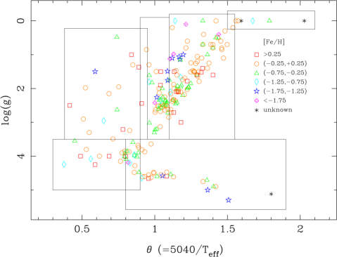
Figure 1: $\log g-\theta$ diagram for the stellar library presented in this work, where $\theta=5040/T_{\rm eff}$. Different symbols are used to indicate stars of different metallicities, as shown in the key. The boxes display the regions of the corresponding local fitting functions for the new CO index (see § 6.2.2 for details).

We have observed a new stellar library in the K band which comprises 220 stars. The observed sample is a subset of MILES (Medium-resolution Isaac Newton Telescope Library of Empirical Spectra; Sánchez-Blázquez et al., 2006; Cenarro et al., 2007), a stellar library in the optical range with well known atmospheric parameters for all the stars (Cenarro et al., 2007). Our final stellar sample includes stars in the following stellar parameter ranges:

$2485\leavevmode\nobreak\ {\rm K}\leq T_{\mathrm{eff}}\leq 13404\leavevmode\nobreak\ {\rm K}$,

$-0.34\;{\rm dex}\leq\log g\leq 5.30\;{\rm dex}$,

$-2.63\;{\rm dex}\leq[{\rm Fe/H}]\leq+0.98\;{\rm dex}$,

where $[{\rm Fe/H}]=\log Z-\log Z_{\odot}$.

This library clearly has a larger metallicity coverage than the previous ones (see Table 1 and Fig. 2 for a comparison between different works), and contains 8 stars in common with KH86, 23 with Wallace & Hinkle (1997) and 39 with Ivanov et al. (2004).

Figure 2: Stellar parameter coverage in the stellar libraries of KH86, Wallace & Hinkle (1997), Ivanov et al. (2004), and this new library. We present separately dwarf and giant (and supergiant) stars (upper and lower panels, respectively). The stellar parameters of the stars from KH86 and Wallace & Hinkle (1997) were taken for Cayrel de Strobel et al. (2001) if available. Otherwise, we assigned solar metallicity and T_eff from their spectral type following the tables of Lang (1991) (small asterisks).

2.3 Observations and data reduction

Table 2: Observational configurations.

Telescope	CAHA 3.50 m	TNG 3.56 m
Instrument	$\Omega$-CASS	NICS
Slit width (″)	0.60	0.75
Grism	#1	KB
Filter	K	–
Spectral coverage	2.01–2.43 $\mu$m	1.95–2.34 $\mu$m
Dispersion	2.527 Å/pix	4.375 Å/pix
FHWM	6.8 Å	11.3 Å
Detector	Hawaii-I	Hawaii-I

The bulk of the stellar library (217 stars) was observed during a total of 13 nights in five observing runs from 2002 to 2005 on the 3.5 m telescope at Calar Alto Observatory (CAHA, Almería, Spain) with $\Omega$–CASS. A subsample of the stellar library (52 stars) was observed again at the Telescopio Nazionale Galileo (TNG) at Roque de los Muchachos Observatory (La Palma, Spain) with NICS (Near Infrared Camera Spectrometer) in February 2006 and May 2007, plus 3 new stars. The details of the instrumental configuration for both runs are given in Table 2.

Each star was observed several times at different positions of the slit (standard procedure for infrared observations) to perform a reliable sky subtraction. Halogen lamps (on and off) and arc lamps were observed for flat-fielding, and C-distortion correction and wavelength calibration, respectively. Vega type (A0) stars were observed at different airmasses during each night in order to calibrate in relative flux and eliminate telluric lines in the stellar spectra.

We carried out a standard data reduction in the infrared using REDucm E (Cardiel, 1999), a reduction package which allows a parallel treatment of data and error frames. The reduction process includes flat-fielding, sky subtraction by subtracting consecutive images (A–B), cosmetic cleaning, C-distortion correction and wavelength calibration with arc lamps, spectrum extraction and relative flux calibration. Atmospheric extinction was corrected by using extinction coefficients (namely the relative contributions of the Raleigh scattering and the aerosol extinction) derived for CAHA Observatory by Hopp & Fernández (2002). Those coefficients were extrapolated for La Palma Observatory to correct the stars observed in this observatory.

Some of the reduction steps that requires more careful work are explained in detail in the following subsections.

2.3.1 Wavelength calibration

Arc spectra of Argon lamps were acquired to perform the C-distortion correction and the wavelength calibration. Due to instabilities and flexures of the instrument and the telescope, calibration arc frames were obtained after each star observed at CAHA. In the K band, the typical number of known lines in the arc spectrum is rather low (just six in our instrumental configuration). Because of that, the wavelength calibration was not accurately enough and a second order wavelength correction was performed by identifying OH air-glow lines in the sky spectrum of each star (Oliva & Origlia, 1992; Rousselot et al., 2000). For observations at CAHA, a polynomial fit of the differences between the observed and theoretical OH lines for the sky spectrum was necessary. The wavelength calibration polynomial is expressed as a function of position as

$$W\left(x\right)=\lambda\left(x\right)+z\left(\lambda\left(x\right)\right),$$ (1)

being $\lambda\left(x\right)$ the initial approximation to the wavelength calibration

$$\lambda\left(x\right)=\sum_{i=0}^{n}a_{i}x^{i},$$ (2)

where $x$ is the position in the spectral direction, and $a_{i}$ are the coefficients of the $n^{\rm th}$-degree calibration polynomial. The second order correction is given by

$$z\left(\lambda\left(x\right)\right)=\sum_{j=0}^{m}b_{j}\lambda^{j},$$ (3)

where $z\left(\lambda\right)$ are the computed differences between the observed and theoretical OH lines, and $b_{j}$ are the coefficients of a $m^{\rm th}$-degree polynomial. In our case, it is a second order polynomial. The final wavelength calibration polynomial correction is

$$z\left(x\right)=\sum_{j=0}^{m}b_{j}\Big{(}\sum_{i=1}^{n}a_{i}x^{i}\Big{)}^{j}=\sum_{k=0}^{l}c_{k}x^{k},$$ (4)

where $c_{k}$ are the coefficients of the new correction polynomial of order $l=m\cdot n$ as a function of the position $x$.

In the case of the observations at the TNG, we compared the observed sky spectrum with the well calibrated sky spectrum from CAHA and we observed constant wavelength differences between them. We cross-correlated both spectra and we applied this constant shift to the wavelength calibration of TNG spectra.

Finally, we checked the final spectra with K band spectra from KH86 and Wallace & Hinkle (1997), since they used a Fourier transform spectrometer, which implies a very accurate wavelength calibration of the spectra. Although in the case of observations at CAHA no differences were obtained, for the TNG observations we had to apply a constant shift in order to achieve the correct wavelength calibration. The origin of this discrepancy is found in the lack of OH sky lines in the reddest wavelength region of the K band, which prevented from an accurate cross-correlation of the sky spectra in that region.

2.3.2 Flux calibration and telluric correction

Figure 3: Upper panel: Histogram with the different $K$ factors (see Eq. 5) employed to correct a particular stellar spectrum from telluric absorptions. Lower panel: Example of a flux standard spectrum before (dotted line) and after (solid line) telluric correction (see details in the text).

There are two ways of flux calibrating infrared spectra. The first method consists of observing a solar type star close to the star to be calibrated. The solar type star is reduced as usual, dividing the final spectrum by the solar spectrum (Livingston & Wallace, 1991) degraded to the same spectral resolution as the problem star. In this way, a spectrum with the information about the response curve and the telluric lines is obtained. This spectrum is then rectified by the ratio between the blackbody spectra at the temperature corresponding to the solar type star and the solar temperature in order to obtain the correct continuum. This final spectrum is used to (relative) flux calibrate and carry out the telluric correction in the stars to be calibrated. The advantage of this method is that it is easy to find a star of this type for each observation.

A second method consists in the observation of Vega type stars at different airmasses during the night. The main reason for choosing these stars is that they are known to have no relevant features in our observational window, except the Br $\gamma$ line. After wavelength calibration, Vega type stars are divided by the well known theoretical Vega spectrum in our spectral range. In that way, a spectrum with both the response curve and the telluric corrections is obtained. The final stellar spectrum is then obtained after dividing each star by this spectrum. In this work, we have used this second approach.

2.3.3 Second order telluric correction

As we mentioned in the previous section, we used the flux standard star in order, not only to flux calibrate the stellar spectra, but also to correct simultaneously for the telluric absorption lines. Due to the variability of the observing conditions during the night, some telluric lines are badly corrected by applying the response curve derived from the flux standard star. For that reason an extra correction was necessary. First of all, we computed a reference spectrum with the information of the telluric lines. For observations at CAHA, we checked the response curves for each night looking for the spectrum with the best removal of telluric features. The ratio between each response curve and the previous spectrum free from telluric contamination provides the telluric spectra that we used to correct all the stellar spectra. In the case of the TNG observations, the telluric spectrum was obtained by dividing the flux standard spectra at high and low airmasses, observed during each night. The telluric spectrum in both observatories, obtained as explained above, consists mainly of differences in the strength of the telluric absorption lines. To correct for these lines, we modified their intensity by multiplying by an adjustable factor $K$, i.e.,

$$S_{K}=\left(S_{0}-1\right)\times K+1,$$ (5)

where $S_{0}$ is the telluric spectrum, and $S_{K}$ is the telluric spectrum adjusted to correct a specific stellar spectrum. We divided the latter stellar spectrum by $S_{K}$ and computed the r.m.s. in the corrected spectrum. The best correction factor, $K$, is the one which minimizes the r.m.s. This method was applied to different identified telluric lines separately, since they do not vary in the same way. This effect can be seen in the histogram of Fig 3, top panel, where the number of telluric lines corrected by a factor $K$ for a given spectrum is represented. In Fig. 3, bottom panel, we present an example of the telluric lines correction for a given flux standard spectrum. Notice that the telluric absorption lines can be present even after flux calibration and it is important to correct them in infrared spectroscopy.

3 Index definitions for the CO band at 2.3 $\mu$m

3.1 The K band region

The most prominent features in the K band are due to the rotational-vibrational transitions of the CO molecule around 2.3 $\mu$m. Important absorptions are also produced by other metallic species, such as Na I, Fe I, Ca I and Mg I (KH86, see Table 3). The only hydrogen line in this spectral range, Br $\gamma$, is present generally in absorption in O and B stars, going into emission for high-luminosity stars (for a detailed study of this kind of stars, see Hanson et al., 1996).

In this paper, we focus our study on the first CO bandhead at 2.29 $\mu$m. Contrary to the Ca I and Na I, the contribution of other species to the CO absorption is almost negligible (see Wallace & Hinkle, 1996; Ramirez et al., 1997, for a further discussion).

Table 3: Main spectroscopic features in the K band (from Kleinmann & Hall, 1986).

Species	$\lambda$	Transition	Lower state
	($\mu$m)		energy (eV)
H I Br $\gamma$	2.1661	$4^{2}F^{0}-7^{2}G$	12.70
Na I	2.2062	$4s^{2}S_{1/2}-4p^{2}P^{0}_{1/2}$	3.19
Na I	2.2090	$4s^{2}S_{1/2}-4p^{2}P^{0}_{3/2}$	3.19
Fe I	2.2263	$x^{5}F^{0}_{4}-e^{5}D_{3}$	5.07
Fe I	2.2387	$x^{5}F^{0}_{3}-e^{5}D_{2}$	5.04
Ca I	2.2614	$4d^{3}D_{3,2,1}-4f^{3}F^{0}_{4}$	4.68
Ca I	2.2631	$4d^{3}D_{3,2,1}-4f^{3}F^{0}_{3}$	4.68
Ca I	2.2657	$4d^{3}D_{3,2,1}-4f^{3}F^{0}_{2}$	4.68
Mg I	2.2814	$4d^{3}D_{3,2,1}-6f^{3}F^{0}_{2,3,4}$	6.72
$\@element[12]{\mathrm{CO}}$(2,0)	2.2935	(2,0) bandhead	0.62
$\@element[12]{\mathrm{CO}}$(3,1)	2.3226	(3,1) bandhead	0.86
$\@element[13]{\mathrm{CO}}$(2,0)	2.3448	(2,0) bandhead	0.32
$\@element[12]{\mathrm{CO}}$(4,2)	2.3524	(4,2) bandhead	1.12

3.2 Previous definitions

In order to measure the CO absorption at 2.3 $\mu$m in an objective way, several authors have proposed different index definitions. Baldwin et al. (1973) suggested a photometric system to measure the CO features based on two narrow filters ($\Delta\lambda=0.10\,\mu$m) centered at 2.30 $\mu$m and at 2.20 $\mu$m for the CO absorption and the continuum, respectively. The CO index was defined as the difference of the two filters relative to the values obtained for $\alpha$ Lyrae, in magnitudes. Following this idea, Frogel et al. (1978) defined the most used photometric CO index (CO_phot), with slightly different filter parameters ($\Delta\lambda=0.08\,\mu$m, for the CO filter centered at 2.36 $\mu$m, and $\Delta\lambda=0.11\,\mu$m for the filter centered at 2.20 $\mu$m for the continuum estimate).

The first spectroscopic CO index (${\rm CO}_{\rm KH}^{\rm mag}$) for the CO(2,0) bandhead at 2.3 $\mu$m was defined by KH86 as

$${\rm CO_{KH}^{mag}}=-2.5\log\;{\rm CO_{KH}}=-2.5\log\;\frac{{\cal F}_{a}}{{\cal F}_{c}},$$ (6)

where ${\rm CO_{KH}}={\cal F}_{a}/{\cal F}_{c}$ is the ratio between the fluxes integrated over narrow wavelength ranges centered in the absorption line ($\lambda\lambda 2.29305-2.29832\leavevmode\nobreak\ \mu$m) and the nearby continuum ($\lambda\lambda 2.28728-2.29252\leavevmode\nobreak\ \mu$m), measured in magnitudes. These band limits have been used to measure the index as an equivalent width (e.g. Origlia et al., 1993). Both measurements can be converted using (Origlia & Oliva, 2000)

$${\rm CO_{KH}^{mag}}=-2.5\log\left(1-\frac{{\rm W}_{\lambda}\left(2.29\right)}{53\AA}\right),$$ (7)

where ${\rm CO_{KH}^{mag}}$ is the spectroscopic index initially defined by KH86 measured in magnitudes, and ${\rm W_{\lambda}\left(2.29\right)}$ is the same index measured as an equivalent width.

Doyon et al. (1994) studied the behaviour of CO_phot and indicated several reasons to introduce their new spectroscopic definition

$${\rm CO_{sp}}=-2.5\ \log<R_{2.36}>,$$ (8)

where $<R_{2.36}>$ is the mean value of the rectified spectrum (normalized in the continuum) in the $2.31-2.40\leavevmode\nobreak\ \mu$m range. This rectified spectrum is obtained by fitting the continuum in the $2.00-2.29\leavevmode\nobreak\ \mu$m range with a power law (F${}_{\lambda}\varpropto\lambda^{-\alpha}$), due to the similarity of the stellar spectrum in the K band to a Rayleigh–Jeans law. As Origlia & Oliva (2000) indicated, this index is just the equivalent width over the CO range relative to a continuum which is extrapolated from shorter wavelengths. As a main advantage, this definition allows measurements of the CO even from poor quality spectra.

Other authors (for example, Lançon & Rocca-Volmerange, 1992; Ramirez et al., 1997; Förster Schreiber, 2000) proposed their own definitions, adopting the bandpasses for the absorption and the continuum without considering the use of those definitions in general situations. Recently, Riffel et al. (2007) measured the CO absorption at 2.3 $\mu$m as an equivalent width between $\lambda\lambda 2.2860-2.3100$ $\mu$m, computing a continuum defined as a spline using points free from emission/absorption lines in the broad interval $\lambda\lambda 2.2350-2.3690$ $\mu$m.

After a study of different band limits for the CO index measured in terms of equivalent widths for stars of different spectral type, Puxley et al. (1997) proposed to extend the absorption band of KH86 up to the end of the CO (2,0) band (2.320 $\mu$m), and the use of three different bands to estimate the continuum ($\lambda\lambda 2.253-2.261\leavevmode\nobreak\ \mu$m, $2.270-2.278\leavevmode\nobreak\ \mu$m and $2.285-2.291\leavevmode\nobreak\ \mu$m). Note that this type of index definition is what Cenarro et al. (2001a) called a generic index. Puxley et al. (1997) adopted this definition because it allows to distinguish between giant and supergiant stars and the correction for velocity dispersion is smaller than with the other definitions.

An additional definition was introduced by Frogel et al. (2001), in which the CO absorption feature is measured using multiple bandpasses to estimate the pseudo-continuum level.

Table 4: Spectroscopic CO index definitions. References are CO${}_{\rm KH}^{\rm mag}$ (Kleinmann & Hall, 1986), I_Puxley (Puxley et al., 1997) and I_Frogel (Frogel et al., 2001). Wavelengths are in vacuum.

Index	Continuum	Absorption	Comments
	bands ($\mu$m)	bands ($\mu$m)
CO${}_{\rm KH}^{\rm mag}$	2.2873–2.2925	2.2931–2.2983	Color-like index
IPuxley	2.2530–2.2610	2.2931–2.3200	Generic index
	2.2700–2.2780
	2.2850–2.2910
IFrogel	2.2300–2.2370	2.2910–2.3020	Generic index
	2.2420–2.2580
	2.2680–2.2790
	2.2840–2.2910
DCO	2.2460–2.2550	2.2880–2.3010	Generic
	2.2710–2.2770		discontinuity

3.3 New index definition

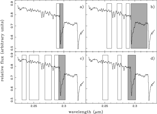
Figure 4: Limits of the bandpasses in the definitions for the CO index proposed by: a) KH86; b) Puxley et al. (1997); c) Frogel et al. (2001); and d) the new CO index presented in this work. Grey and open bands represent absorption and continuum bandpasses, respectively, for each index definition, superimposed on the spectrum of HD137704.

Even though the number of different CO index definitions is large, we have explored in detail whether any of these is actually well suited for a practical study of this spectroscopic feature in the integrated spectra of galaxies. Curiously, from the list of previous index definitions only the one presented by Puxley et al. (1997) (based on the previous definition by KH86) was designed taking into account the variations of the index with radial velocity and velocity dispersion, both of them very important in the study of galaxies. In this work we have spent an additional effort to investigate the possibility of finding an optimal CO index definition that could improve all the previous definitions.

In order to carry out this task, we have focused our efforts on defining a CO index which is less sensitive to low signal-to-noise ratios, degradation due to spectral resolution and/or velocity dispersion, and errors in wavelength calibration (or errors in radial velocity), and in relative flux calibration (see the next sections for a further study of each case).

After exploring different possibilities for the definition of the new index, we propose to measure the CO at 2.29 $\mu$m as a generic discontinuity, i.e., as the ratio between the average fluxes in the continuum and in the absorption bands

$${\rm D_{generic}}\equiv\frac{\frac{\displaystyle\sum_{i=1}^{n_{c}}{\int_{\lambda_{c,i_{1}}}^{\lambda_{c,i_{2}}}F_{c,i}\left(\lambda\right)\;\mbox{d}\lambda}}{\displaystyle\sum_{i=1}^{n_{c}}{(\lambda_{c,i_{2}}-\lambda_{c,i_{1}})}}}{\frac{\displaystyle\sum_{i=1}^{n_{a}}\int_{\lambda_{a,i_{1}}}^{\lambda_{a,i_{2}}}F_{a,i}\left(\lambda\right)\;\mbox{d}\lambda}{\displaystyle\sum_{i=1}^{n_{a}}{(\lambda_{a,i_{2}}-\lambda_{a,i_{1}})}}}$$ (9)

where ${\rm D_{generic}}$ is the generic discontinuity, and $F_{a,i}\left(\lambda\right)$ and $F_{c,i}\left(\lambda\right)$ are the flux in the $n_{a}$ absorption bands and $n_{c}$ continuum bands, respectively. Finally, $\lambda_{x,i_{1}}$ and $\lambda_{x,i_{2}}$ are the lower and upper wavelength limits of the $i^{\rm th}$ band $x$ (where $x$ is $a$ or $c$). This new definition is similar to the B4000 index defined by Gorgas et al. (1999) but using more than one bandpass to define the continuum and the absorption regions.

Here we propose to measure the CO feature at $2.3\mu$m as a generic discontinuity, D_CO, using two bandpasses for the continuum ($n_{c}=2$) and one bandpass for the absorption region ($n_{a}=1$). The limits of these bands are also listed in Table 4. We selected the number of bandpasses and their location taking into account several factors. Concerning the continuum bandpasses, we have eluded the Ca I and Mg I features, trying not to extend too far towards shorter wavelengths in order to avoid potential systematic effects arising in the flux calibration of wide line-strength indices. In the case of the absorption region, one single bandpass is enough to cover the first CO bandhead. Compared with previous definitions, we decided to shift slightly the blue continuum bandpass limit to obtain an index which is more stable with velocity dispersion (i.e. spectral resolution) and with radial velocity uncertainties.

Following Cardiel et al. (1998), it is not difficult to show that the expected variance in a D_generic index can be computed as

$$\sigma^{2}[{\rm D}_{\rm generic}]=\frac{{\cal F}_{c}^{2}\sigma_{{\cal F}_{a}}^{2}+{\cal F}_{a}^{2}\sigma_{{\cal F}_{c}}^{2}}{{\cal F}_{a}^{4}},$$ (10)

where ${\cal F}_{x}$ is the total flux per wavelength unit in the continuum ($x=c$) and the absorption ($x=a$) region, determined from the coaddition of the flux in all the corresponding bandpasses, i.e.,

$${\cal F}_{x}\equiv\Theta\;\frac{\displaystyle\sum_{i=1}^{n_{x}}\sum_{k=1}^{N_{\rm pixels}^{i}}F_{x,i}\left(\lambda_{k}\right)}{{\displaystyle\sum_{i=1}^{n_{x}}{(\lambda_{x,i_{2}}-\lambda_{x,i_{1}})}}},$$ (11)

being $n_{x}$ the number of bandpasses in either the continuum or the absorption region, $\Theta$ is the linear dispersion (in Å/pixel), $N_{\rm pixels}^{i}$ is the number of pixels covered by the $i^{\rm th}$ bandpass of the $x$ region (with $x$ equal to $c$ or $a$), and $\lambda_{k}$ is the central wavelength of the $k^{\rm th}$ pixel. The variance in these total fluxes are simply computed as the quadratic sum of the individual variances in each pixel, i.e.,

$$\sigma^{2}_{{\cal F}_{x}}=\Theta^{2}\frac{\displaystyle\sum_{i=1}^{n_{x}}\sum_{k=1}^{N_{\rm pixels}^{i}}\sigma^{2}_{F_{x,i}}\left(\lambda_{k}\right)}{\left[{\displaystyle\sum_{i=1}^{n_{x}}{(\lambda_{x,i_{2}}-\lambda_{x,i_{1}})}}\right]^{2}},$$ (12)

where, in particular, $\sigma^{2}_{F_{x,i}}\left(\lambda_{k}\right)$ is the variance corresponding to the random error in the $k^{\rm th}$ pixel. It is important to highlight that in these expressions we are assuming that the random errors in each pixel are not correlated.

3.4 Sensitivities of the indices to different effects

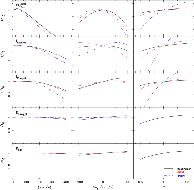
Figure 5: Study of the sensitivity of the different CO index definitions (from top to bottom, CO${}_{\rm KH}^{\rm mag}$, I_Puxley, I_Frogel, D_Frogel and D_CO) to several relevant parameters. Left column: ratio between the index I measured on the spectra broadened with a given $\sigma$, and the index I₀ measured on the initial spectra ($\sigma_{0}=3$ km/s, corresponding to the resolution of the stellar library of Wallace & Hinkle, 1996). Central column: ratio between the index I for a given v_r and the index I₀ in the original spectrum (v${}_{\rm r}=0$ km/s). Right column: ratio between the index I measured on the spectrum multiplied by a curved spectrum parametrized by $\beta$ (see § 3.4.3 for details) and the index measured over the original spectrum, I₀, as a function of the curvature parameter $\beta$.

In this section, we discuss the sensitivity of previous spectroscopic indices defined by KH86 (CO${}_{\rm KH}^{\rm mag}$), Puxley et al. (1997) (I_Puxley) and Frogel et al. (2001) (I_Frogel), and the new CO index (D_CO) to velocity dispersion (or spectral resolution), wavelength calibration (radial velocity), relative flux calibration and signal-to-noise (S/N) ratio. A fifth index, D_Frogel, is considered: a generic discontinuity based on the same bands proposed by Frogel et al. (2001). In Fig. 4 we show the bandpasses for these index definitions. For this study, we selected from the high resolution library of Wallace & Hinkle (1996) three stars with similar spectral type (M2–5; chosen because of their strong CO features) and different luminosity class (supergiant, giant and dwarf) in order to account for differences depending on the type of star. The resolution of the spectra is 0.54 Å(FHWM) and they are all shifted to rest-frame.

3.4.1 Spectral resolution and velocity dispersion broadening

In order to study the sensitivity of the spectroscopic CO indices to the spectral resolution or velocity dispersion broadening ($\sigma$), we broadened the stellar spectra of the selected stars with additional $\sigma$’s from the initial $\sigma_{0}$ up to $\sigma=400$ km/s (in steps of 10 km/s). The different indices were measured on all these broadened spectra and we computed the ratio between the index (I) at each $\sigma$ and the index measured on the original spectrum (I₀). Fig. 5 (left column) shows this ratio as a function of the velocity dispersion for the definitions we are studying. Compared to the other index definitions, the two generic discontinuities (D_Frogel and D_CO) are clearly the less sensitive to velocity dispersion broadening.

3.4.2 Wavelength calibration

Sometimes, errors in the wavelength calibration arise in the spectra even after a very careful reduction or due to an inaccurate radial velocity (v_r) estimate of the studied object. Because of that, it is important to define indices with the least possible sensitivity to this kind of uncertainties. To quantify this effect, we measured the CO absorption with the different index definitions in the stellar spectra shifted from $-200$ to $+200$ km/s with steps of 4 km/s in radial velocity. In Fig. 5 (central column) we present the ratio between the index, I, measured at v_r and the initial value I₀ (assumed v${}_{\rm r}=0$ km/s) as a function of the considered v_r for different types of stars. It is apparent from the figures that the indices CO${}_{\rm KH}^{\rm mag}$, I_Puxley and I_Frogel are very sensitive to radial velocity uncertainties, while D_Frogel and the new index definition D_CO are more robust to this effect.

3.4.3 Flux calibration

As we explained in § 2.3.2, it is common to use theoretical spectra to recover the real shape of the continuum. This practise implies the knowledge of the temperatures of the standard stars. For that reason, we have studied the impact, during flux calibration, of an error in the temperature estimate of the standard stars. To analyse the impact when solar-type stars are used as flux standards, we computed the blackbody spectrum in the interval $5600\leq T_{\mathrm{eff}}\leq 6300$ K, and derived the ratio between these spectra and the blackbody, at solar temperature. To study the effect when Vega type stars are used as calibrators, we analysed the differences from the theoretical spectrum of Vega ($T_{\mathrm{eff}}\sim 9400$ K) and the real temperature of the Vega type stars (from 8400 to 14400 K for our study). In both cases, we found that the changes in the continuum produced by differences in the assumed temperature of standard stars produce negligible differences in the measured indices.

Finally, we studied the impact of a wrong curvature in the response curve, which is a typical source of systematic error. In order to obtain an estimate of this effect, as a first order approach we have artificially modified the continuum shape of the original spectra by multiplying them by a second order polynomial. This polynomial was chosen to pass through 3 fixed points, two at the borders of the wavelength range (where the polynomial were forced to be equal to 1.0), and another point at the center of that range (where the polynomial was set to a variable parameter $\beta$ ranging from 0.5 to 1.5). In Fig. 6 we show different examples of these polynomials for distinct values of $\beta$. Note that, with this exercise, we simply studied the effect of a low frequency error in flux calibration.

In Fig 5 (right column) we present the ratio between the measured index in the stellar spectrum multiplied by the polynomial for a given value of $\beta$, I, and the original one, i.e., I₀ for $\beta=1.0$ (no additional curvature), as a function of the parameter $\beta$. The sensitivity of each index definition to the $\beta$ parameter is, not surprisingly, dependent on the location and wavelength coverage of the index bandpasses, and also depends on the way the pseudo-continuum is determined, and the absolute value of the index. For these reasons, CO${}_{\rm KH}^{\rm mag}$, I_Puxley and I_Frogel are the most sensitive to an error in the response curve. In particular, the CO${}_{\rm KH}^{\rm mag}$ depends strongly on the strength of the CO absorption. On the other hand, I_Puxley and I_Frogel, defined as generic indices, extrapolate the continuum value into the absorption band and, in that way, the wrong curvature too. In addition, the generic discontinuities D_Frogel and D_CO, computed as the averaged flux in the continuum and absorption bands, exhibit no differences between dwarf, giant and supergiant stars.

Figure 6: Examples of the curved spectra used in the study of the sensitivity of the different index definition to a wrong curvature of the spectrum. The parameter $\beta$ determines the distance to the maximum/minimum in the center of the spectrum (shown here for the polynomial displayed with a solid line).

3.4.4 S/N ratio

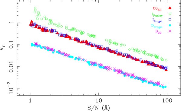
Figure 7: Example of the study of the dependence of the relative error in the measure of the first CO bandhead using different index definitions at a given S/N ratio per Å. We represent the relative errors vs. S/N ratio (in logarithmic scale) measured on the simulated spectra of a giant star (the results are independent of the type of star). Different symbols are used to indicate different index definitions, as shown in the key. See text for details.

One important issue to take into account in the definition of a new index is the dependence of the relative error of the measurements on the S/N ratio. In this sense, the aim is to find an index definition which provides the lowest relative error in the measurements with the lowest signal-to-noise ratio in the spectra. For that reason, we have studied the behaviour of relative errors measured with previously analyzed CO index definitions as a function of the S/N ratio. Using a particular stellar spectrum, we have simulated a set of one hundred spectra (and their associated error spectra) with random S/N(Å) ratios in the range 1.0–100.0. For this task we have used the program indexf (Cardiel, 2007). In Fig 7 we compare the results obtained for a giant star (same results are obtained for supergiant and dwarf stars). Not surprisingly, the relative errors in all the definitions follow

$$\varepsilon_{\rm r}=\frac{c}{\rm S/N(\AA)},$$ (13)

where $c$ is a constant that depends on the particular index. This result was already found for atomic and molecular indices (Cardiel et al., 1998), and for generic indices (Cenarro et al., 2001a). It is clear from Fig. 7 that the same holds for generic discontinuities. Considering Eq. 13, it is evident that, at a given S/N ratio, the lower relative errors correspond to the index definitions with lower $c$ values. Table 5 list these values for the five index definitions under study. From these numbers and the data displayed in Fig. 7, it is obvious that D_CO is comparable to D_Frogel, while CO${}_{\rm KH}^{\rm mag}$, I_Puxley and I_Frogel provide larger relative errors for a given S/N ratio.

Table 5: Values of the constant $c$ of Eq. 13 for the different index definitions analyzed in § 3.4.

Index	$c$
CO${}_{\rm KH}^{\rm mag}$	$0.7537$
IPuxley	$2.0258$
IFrogel	$0.8123$
DFrogel	$0.1075$
DCO	$0.1198$

3.4.5 The best index definition

Once we have studied the behaviour of the different CO index definitions as a function of all the relevant parameters, we can conclude that the D_CO index definition is, in general, preferable.

On one hand, CO${}_{\rm KH}^{\rm mag}$, I_Frogel and I_Puxley are too sensitive of spectral resolution and errors in wavelength calibration and radial velocity. In addition, the behaviour of CO${}_{\rm KH}^{\rm mag}$, I_Frogel and I_Puxley are also too sensitive to uncertainties in the spectrophotometric system (i.e., flux calibration).

When the sensitivity to S/N is included in the comparison, it is clear that the best definitions are the two generic discontinuities, namely D_Frogel and D_CO. Since the use of generic discontinuities for measuring the CO absorption is introduced for the first time in this paper, and considering that the D_CO is practically insensitive to spectral resolution (or velocity dispersion broadening) up to $\sigma\sim 400$ km/s, we propose to use the new definition, especially for the future analysis of integrated spectra.

3.5 Conversion between different CO index systems

Figure 8: Comparison between measurements on the TNG subsample of the first CO bandhead using different index definitions. The panels show the transformation between the new index D_CO and CO${}_{\rm KH}^{\rm mag}$, I_Frogel, I_Puxley and CO_KH (from top to bottom, and from left to right). The solid lines are least squares fits to the data, and correspond to the transformations given in Eqs. 14–17.

In this section we give the calibrations to convert between the new CO index definition and the CO indices defined by KH86, Puxley et al. (1997) and Frogel et al. (2001). In order to obtain these conversions, we have measured the indices on the subsample of stars observed at the TNG ($3200\leq T_{\mathrm{eff}}\leq 9625$ K, $0.00\leq\log g\leq 5.00$, $-1.73\leq[{\rm Fe/H}]\leq+0.36$). The calibrations were computed by deriving a least squares fit to the data. The fits are completely compatible with index measurements on the KH86 and Wallace & Hinkle (1997) spectra which are on the same spectrophotometric system. Just six stars from Wallace & Hinkle (1997) deviate more than $3\sigma$ from the fitted relation due to a problems in the continuum and the telluric correction of those spectra. In Fig. 8 we show all these fits and the data used to compute them.

The conversion between the index defined by KH86, ${\rm CO_{KH}^{mag}}$, and the new index D_CO is given by

$${\rm D_{CO}}=1.0407\left(\pm 0.0021\right)+0.2317\left(\pm 0.0035\right)\;{\rm CO_{KH}^{mag}}$$ (14)

with $r^{2}=0.9863$.

The expression to compute D_CO from the index defined by Frogel et al. (2001) is

$${\rm D_{CO}} = 1.0507\left(\pm 0.0031\right)+0.0077\left(\pm 0.0005\right)\;{\rm I_{Frogel}}+$$ (15)

$$+0.00007\left(\pm 0.00002\right)\;{\rm I_{Frogel}^{2}}$$

with $r^{2}=0.9802$, where ${\rm I_{Frogel}}$ is measured as an equivalent width (Å).

As we mentioned before, ${\rm I_{Puxley}}$ is also measured as an equivalent width. The expression to compute the D_CO index from I_Puxley is

$${\rm D_{CO}}=1.0488\left(\pm 0.0033\right)+0.0051\left(\pm 0.0001\right)\;{\rm I_{Puxley}}$$ (16)

with $r^{2}=0.9629$.

Finally, we have also computed the conversion between the ratio CO_KH (not to be confused with CO${}_{\rm KH}^{\rm mag}$; see Eq. 6) and the new CO index

$${\rm D_{CO}} = 2.1119\left(\pm 0.0724\right)-1.6205\left(\pm 0.1772\right)\;{\rm CO_{KH}}+$$ (17)

$$+0.5521\left(\pm 0.1071\right)\;{\rm CO_{KH}^{2}}$$

with $r^{2}=0.9867$. This last transformation will be used in next section.

4 Measurements of the CO absorption for the stellar library and error estimates

4.1 Index measurements

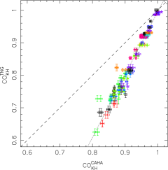
Figure 9: Left panel: CO_KH index measured on the stars with solar metallicity observed at the TNG (CO${}_{\rm KH}^{\rm TNG}$) vs. the same measurements in the most similar stars from the KH86 library (CO_KH). Right panel: CO_KH index measured on stars observed in common at TNG (CO${}_{\rm KH}^{\rm TNG}$) and CAHA (CO${}_{\rm KH}^{\rm CAHA}$). Different symbols are used for distinct observing runs at CAHA, although no segregation of the data between runs is apparent. The dotted line shows the empirical correction for the CAHA measurements. In both panels, the dashed line shows the one-to-one relation.

A detailed study of the continuum in spectra observed at CAHA compared with the the spectra published by KH86 have revealed some problems with the flux calibration of the CAHA data. The shape of the continuum in these spectra showed a spurious and non-reproducible high-frequency structure superimposed to the real continuum, which was affecting not only the shape of the continuum but also the final index measurements. During the reduction of the data it was neither possible to identify nor correct this additional source of noise.

In order to handle, at least in an empirical way, the spectrophotometric calibration of the CAHA spectra, we re-observed a good subsample of the stellar library at the TNG. To guarantee that the TNG data were on the appropriate spectrophotometric system, the CO measurement of each star observed at the TNG was compared with the measurement of the most similar spectrum (in $T_{\mathrm{eff}}$ and luminosity class) available in the KH86 library at the same spectral resolution.

Since the bandpasses for the new index D_CO encompass a wide range in wavelength, the strange behaviour of the continuum shape in the CAHA spectra has a large impact on the index measurements. Luckily, this is not such a big issue for the CO_KH ratio, since both continuum and absorption bandpasses are very close in this definition. For that reason, we decided to measure the CO_KH index, transforming afterward the results into the D_CO index using Eq. 17 (which provides a good conversion between both indices, as shown in the previous section). In more detail, the method to derive the final spectrophotometric calibration can be summarized as follows.

First of all, the CO_KH measurements of the subsample of stars with solar metallicity re-observed at the TNG were compared with the corresponding star in the KH86 library, as explained before. In Fig. 9, left panel, the results of this comparison are shown. A least squares fit to the one-to-one relation was computed, providing $r^{2}=0.9768$. Although some points in this figure appear relatively far from the 1:1 relation (considering their error bars), it is important to highlight that we are not comparing the same stars, and that, in any case, the determination coefficient $r^{2}$ is high enough to guarantee the quality of the transformation.

Finally, we used the stars in common between the TNG and CAHA to empirically correct the measured indices on the CAHA spectra sampled at the spectral resolution of the TNG spectra. Fig. 9, right panel, presents the relation between the CO_KH ratio in common stars observed in both observatories. A least squares fit to a straight line gives $r^{2}=0.9539$. We have checked that a unique empirical correction is valid for all the observing runs at CAHA (within the statistical errors). For this study, we have used all the individual measurements for each star instead of averaging all the observations along the slit. After transforming the CAHA CO_KH measurements onto the correct spectrophotometric system, we applied Eq. 17 to obtain the new D_CO measurements, which will be used later to derive the empirical fitting functions.

4.2 Random errors and systematic effects

4.2.1 Known sources of random errors

We have considered several sources of random errors: photon statistic and read-out noise, errors due to the detector cosmetic, the combined effect of wavelength calibration and radial velocity uncertainties, and flux calibration uncertainties.

(i) Photon statistics and read-out noise. With the aim of tracing the propagation of photon statistic and read-out noise, we followed a parallel reduction of data and error frames with the reduction package REDucm E , which creates error frames at the beginning of the reduction procedure and translates into them, by following the law of combination of errors, all the manipulations performed over the data frames. In this way the most problematic reduction steps (flat-fielding and distortion corrections, wavelength calibration, etc.) are taken into account and, finally, each data spectrum has its corresponding error spectrum which can be used to derive reliable photon errors in the index ($\sigma_{\rm photon}$). A detailed description of the estimate of random errors in the measurement of classical line-strength indices and the impact of their interpretation are shown in Cardiel et al. (1998, 2003). The new CO index is defined in this paper as a generic discontinuity and follows the expressions given in § 3.3 for the errors.

(ii) Errors due to the detector cosmetic. In the case of infrared detectors, the errors due to the detector cosmetic are very important. We measured the r.m.s. (root-mean-squared) on two different regions of the spectra with no apparent absorption features ($\lambda\lambda 2.2685-2.2790$ $\mu$m and $\lambda\lambda 2.2825-2.2890$ $\mu$m), in order to obtain an estimation of photon statistics and read-out noise errors together with the errors due to imperfections present in the images even after flat-fielding correction. In Fig. 10 we compare the errors due to photon statistic and read-out noise errors (upper panel), derived from first principles (using the parallel reduction of data and error frames), with the errors from direct measurement of the r.m.s in the spectra (lower panel). As it can be seen, we are underestimating the random errors if we do not consider the errors due to the detector cosmetic.

Figure 10: Upper panel: Histogram with the photon statistic and read-out noise error in the D_CO for the stars in the stellar library. Lower panel: Similar histogram with the errors derived from measurements of the r.m.s. on two spectral regions with no apparent absorption features for the stars in the stellar library.

(iii) Wavelength calibration and radial velocity errors. The combined effect of wavelength calibration and radial velocity correction is another random source of error. We considered as an upper limit for the wavelength calibration error the projection on the spectral direction of half of the slit width. These values were measured from the FWHM of the arc lines, providing errors of 45 km/s for the observations at CAHA and 85 km/s for the TNG images. These numbers translate into typical errors of $\sigma[{\rm D_{CO}}]=0.002$ and $\sigma[{\rm D_{CO}}]=0.004$, for CAHA and TNG respectively.

Radial velocity for most of the stars in the stellar library were taken from the Hipparcos Input Catalogue (Turon et al., 1992), which in the worst cases are given with mean probable errors of 5 km/s. For the missing stars in this catalogue, we adopted radial velocities from the SIMBAD database, which presents typical errors of a few km/s. These errors are completely negligible in comparison with the wavelength calibration errors already mentioned.

(iv) Flux calibration errors. In order to check for possible random errors in the index measurements due to the flux calibration method, we should have observed several spectrophotometric reference spectra each observing night. Since this is a highly time-consuming approach, we did not observe them. Alternatively, we have decided to check the impact of this kind of error through the comparison of common stars between different nights and runs and we will discuss it in § 4.2.3.

4.2.2 Additional sources of random errors

Expected random errors for each star can be computed by adding quadratically the random errors derived from the known sources previously discussed, i.e.,

$$\sigma^{2}[{\rm CO}]_{\rm initial}=$$ (18)

$$=\sigma^{2}[{\rm CO}]_{\rm photon+cosmetic}+\sigma^{2}[{\rm CO}]_{\rm wavelength}.$$

However, additional (but unknown) sources of random errors may still be present in the data. Using the multiple observations available for each particular star, we compared the standard deviation of the different D_CO measurements ($\sigma[{\rm CO}]_{\rm rms}$) with the initial random error ($\sigma^{2}[{\rm D}_{\rm CO}]_{\rm initial}$) for that star. In the cases in which the standard deviation was significantly larger than the expected error (using a $\chi^{2}$-test of variances), a residual random error $\sigma[{\rm D}_{\rm CO}]_{\rm residual}$ was derived as

$$\sigma^{2}[{\rm CO}]_{\rm residual}=\sigma^{2}[{\rm CO}]_{\rm rms}-\sigma^{2}[{\rm CO}]_{\rm initial},$$ (19)

and quadratically added to the initial random errors to obtain the final random errors, i.e.,

$$\sigma^{2}[{\rm CO}]_{\rm final}=\sigma^{2}[{\rm CO}]_{\rm initial}+\sigma^{2}[{\rm CO}]_{\rm residual}.$$ (20)

It is worth noting that this additional error was only necessary for a few stars, since most of them presented consistent errors between different measurements.

4.2.3 Systematic effects

Due to the large number of runs needed to complete the whole library, systematic errors can arise because of possible differences between the spectrophotometric systems of each run at both the CAHA and TNG telescopes. To guarantee that the whole dataset is on the same system, we observed stars in common between different runs at each telescope. We compared the index measurements of these stars by applying a $t$-test to study whether the differences of the index measurements of the common stars were statistically larger than zero, finding no systematic effects between different nights within a given observing run, and between different runs. For that reason we have considered that an additional error exclusively due to flux calibration was not required (i.e., the actual flux calibration errors are within the already computed random errors).

It is important to highlight that there is not guarantee that our data are on a true spectrophotometric system, so we encourage readers interested in using our results to include in their observing plan stars in common with the stellar library to ensure a proper comparison.

4.3 Additional measurements of the CO absorption: globular cluster stars

To improve the stellar parameter coverage of our stellar library, additional stars were included for the computation of empirical fitting functions for the D_CO (see § 6). Frogel et al. (2001) and Stephens & Frogel (2004) presented a sample of globular cluster giant stars ($R\sim 1500$, $\sigma\sim 85$ km/s), characterized by their low metallicity, with measurements of the CO absorption at 2.3 $\mu$m using the definition of Frogel et al. (2001). Since there is not dependence of I_Frogel at the spectral resolution of these data (see Fig 5), we transformed their CO measurements to the new index by applying Eq. 15. The stellar atmospheric parameters of these stars were determined from $J$ and $K$ photometry, as it is explained in § 5.2. Finally, we considered 80 stars from Frogel et al. (2001) and 14 stars from Stephens & Frogel (2004), which, together with the stellar library presented in this work, will be used to parametrize the behaviour of the CO index as a function of the stellar atmospheric parameters.

5 Stellar atmospheric parameters

Figure 11: Pseudo-HR diagrams for the cluster stars together with adequate isochrones (Girardi et al., 2000; Lejeune et al., 1997, 1998) for each individual cluster. Open circles are used for individual stars in the clusters. Solid and dashed lines illustrate isochrones of 12.59 Gyr and two metallicity values enclosing the one of the cluster (as shown in the labels). Adopted metallicities for the clusters are labeled in the figure. In all cases, the solid line is employed to indicate the isochrone whose metallicity is closer to that of the cluster. Surface gravity for each star was estimated by comparing to the predicted $M_{K}$ as explained in § 5.2. Final atmospheric parameters for each cluster star, and their corresponding errors, are given in Table LABEL:table_cluster_stars.

In this section, we present the atmospheric parameters for the stars considered in the computation of the empirical fitting functions for the D_CO index presented in § 6.

Figure 12: Behaviour of the first CO bandhead with T_eff, $\log g$ and [Fe/H] (from left to right). In each case, the displayed stars have been selected to exhibit a range in a given atmospheric parameter (as shown in the labels) with similar values for the other two parameters.

5.1 Atmospheric parameters for the observed stellar library sample

As we mentioned before, the stellar library presented in this work is a subsample of the MILES library (Sánchez-Blázquez et al., 2006). Following the previous work by Cenarro et al. (2001b), a reliable and highly homogeneous data set of atmospheric stellar parameters for the stars in MILES library was derived by Cenarro et al. (2007) as the result of a previous, extensive compilation from the literature and a carefully calibration and correction by bootstrapping of the data on to a reference system. In short, the method can be itemized in the following steps (see Cenarro et al. 2001b and Cenarro et al. 2007 for a more detailed explanation of the working procedure): (i) selection of a high-quality, standard reference of atmospheric parameters, (ii) bibliographic compilation of atmospheric parameters of the stars in the library, (iii) calibration and correction of systematic differences between the different sources and the standard reference system, and (iv) determination of averaged, final atmospheric parameters for the library stars from all those references corrected on to the reference system. Together with the atmospheric parameters, an estimation of the uncertainties in their determination is given for each star. In that way, stellar atmospheric parameters (and their uncertainties) are perfectly well known for the stars in the new stellar library.

5.2 Atmospheric parameters for the additional globular cluster stars

For the subsample of 94 red giant branch (RGB) stars from Galactic globular clusters, effective temperatures ($T_{\mathrm{eff}}$) and surface gravities ($\log g$) were derived from $J$ and $K$ photometry, following a technique similar to that explained in Cenarro et al. (2007) (see also Cenarro et al., 2001b). Absolute, reddening corrected photometry for all clusters was taken from Frogel et al. (2001) and Stephens & Frogel (2004).

The surface gravity for each cluster star was estimated by matching its location in a $M_{K}$–$\left(J-K\right)$ diagram to the appropriate isochrones from Girardi et al. (2000) (see Fig. 11), whose colors and magnitudes were previously transformed to the observational plane using the empirical colour-temperature relations for giant stars from Alonso et al. (1999) and Lejeune et al. (1997, 1998), with the latter being for giants with $T_{\mathrm{eff}}\leq 3500$ K (see more details in Vazdekis et al., 2003).

If available, the metallicity for each cluster was taken from the work by Rutledge et al. (1997) (hereafter RHS97), which provides metallicity estimates for Galactic globular cluster on the Carretta & Gratton (1997) (hereafter CG97) scale based on the Ca II triplet strengths of their RGB stars. This was the case for NGC0104, NGC0288, NGC0362, NGC5927, NGC6553, NGC6624, NGC6712, and M69. For M71, however, we kept the value in the CG97 scale inferred by Cenarro et al. (2002) according to the CaT indices of their stars. If not available in RHS97, metallicity values in the (Zinn & West, 1984, hereafter ZW84) scale were transformed into the CG97 scale using Equation 7 in CG97. This was the case for the rest of our GC sample. For NGC6388, NGC6440, Liller1, and Terzan2, ZW84 metallicity values were taken from Table 6 in that paper. For NGC6528, the value given in the 2003 revised version of the catalog of parameters for Milky Way globular clusters (Harris, 1996) was employed. It is important to note that there is a double reason for using the CG97 metallicity scale in this work. First, since, as compared to the Zinn & West (1984) metallicity scale, the agreement between the locus of the cluster RGB stars and the corresponding isochrones in the $M_{K}$–$\left(J-K\right)$ plane is much better when using CG97 values, particularly in the high metallicity regime. Also, because the metallicities of the rest of cluster stars in this paper (as taken from either Cenarro et al., 2001b, 2007) are already on the CG97 scale, thus guaranteeing full consistency among the metallicities of the whole star sample, and minimizing systematics in the computation of the fitting functions.

Assuming that all the galactic globular cluster under study are similarly old, and taking into account the above metallicities, for all the stars in each cluster we used two of the Girardi’s isochrones of 12.6 Gyr with metallicities enclosing the corresponding value of the cluster (solid and dashed lines in Fig. 11). For each isochrone, a $\log g$ value for each star was estimated by interpolating in $M_{K}$. Final $\log g$ values were computed as weighted means of the single values derived from the two different metallicity isochrones, with weights accounting for the differences between the adopted cluster metallicity and the isochrone values.

Effective temperatures for all the cluster giants were computed on the basis of the $\left(J-K\right)$–$T_{\mathrm{eff}}$ relations given in Alonso et al. (1999) (for $T_{\mathrm{eff}}>3500$ K) and Lejeune et al. (1997, 1998) (for $T_{\mathrm{eff}}\leq 3500$ K). Interestingly, since Alonso’s relation for $\left(J-K\right)$ does not depend on either metallicity and $\log g$, $T_{\mathrm{eff}}$ can be directly determined from $\left(J-K\right)$. This indeed helps to minimize the sources of uncertainties in the final temperatures of most globular cluster giants. As a matter of fact, only a few temperatures for very cold stars were computed using Lejeune’s relations.

Errors for the derived atmospheric parameters of the cluster stars were estimated from input uncertainties in [Fe/H] and in the photometric data employed in this technique. For those [Fe/H] values taken from RHS97 and Cenarro et al. (2002), the uncertainties given therein were assumed. For the rest of the clusters, metallicity errors were computed from those given in ZW84 through standard error propagation in Equation 7 of CG97. Since most stars in Frogel et al. (2001) and Stephens & Frogel (2004) were selected from the bright ends of the globular cluster luminosity functions, photometric observational errors in $J$ and $K$ bands turned out to be very small ($<<0.06\,$mag; see e.g. Frogel et al., 1995; Kuchinski et al., 1995; Kuchinski & Frogel, 1995) as compared to typical uncertainties in the assumed distance moduli and reddening corrections. Errors in $M_{K}$, and $\left(J-K\right)$ are therefore strongly dominated by the above effects. For this reason, typical errors of 0.20 mag and 0.06 mag for $M_{K}$ and $\left(J-K\right)$, respectively, have been considered for all the cluster stars.

Final values of $T_{\mathrm{eff}}$, $\log g$, [Fe/H], and their corresponding errors for the whole sample of cluster stars are presented in Table LABEL:table_cluster_stars.

6 Empirical calibration of the new CO index

In this section we parametrize the behaviour of the new CO index in terms of the stellar atmospheric parameters (T_eff, $\log g$ and [Fe/H]. For that purpose, we use the D_CO index measurements of the stars of the new stellar library and on the sample of globular cluster stars from Frogel et al. (2001) and Stephens & Frogel (2004) (see § 4.3). This paper shows a detailed quantitative metallicity dependence of the CO feature at 2.3 $\mu$m.

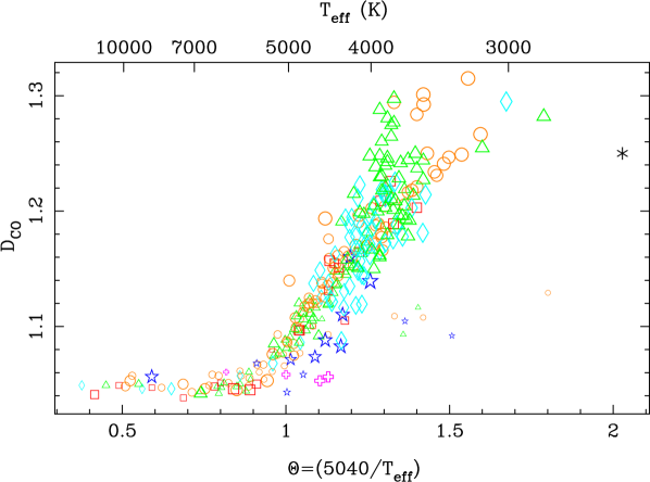
Figure 13: D_CO index as a function of $\theta\,\left(=5040/T_{\mathrm{eff}}\right)$ for the stars of the new library plus the globular cluster stars from Frogel et al. (2001) and Stephens & Frogel (2004) used in this study. Symbols mean metallicity, as explained in Fig. 1. Relative symbol sizes indicate gravity ranges (small symbols for dwarfs, increasing symbol size for decreasing gravity).

6.1 Behaviour of the CO index as a function of stellar atmospheric parameters

The dependence of the strong CO absorption bands as a function of the effective temperature and surface gravity is well known from the first studies in the infrared (KH86, Johnson & Mendez, 1970; Frogel et al., 1978; Lançon & Rocca-Volmerange, 1992; Doyon et al., 1994; Wallace & Hinkle, 1997; Ramirez et al., 1997; Förster Schreiber, 2000; Lançon & Wood, 2000; Ivanov et al., 2004; Silva et al., 2008). The CO absorptions turn deeper as the stars are cooler, while hot stars show no trace of CO features. On the other hand, as surface gravity decreases, the CO absorptions become prominent, i.e., supergiant stars present more important CO absorption than dwarfs. All the previous works in the K band highlighted both the tight correlation of their defined CO indices with temperature (spectral type or $J-K$ color in the first papers), and the dependence of the CO absorption with surface gravity. In addition, a few theoretical studies (McWilliam & Lambert, 1984; Origlia et al., 1993) indicate that these spectroscopic features should be metallicity dependent. Terndrup et al. (1991) showed that Baade’s window stars have deep 2.3 $\mu$m bands, what they interpreted as these stars probably having a high metallicity. Model predictions by Maraston (2005) also showed the dependence of the CO absorptions in the K band with metallicity. Observations of composite stellar population (e.g. Origlia & Oliva, 2000; Riffel et al., 2007) give support to this dependence. Unfortunately, the lack of empirical stellar libraries with an appropriate coverage in metallicity had prevented, until now, a detailed quantitative description of this dependence. Fig. 12 shows, graphically, how the first CO bandhead at 2.3 $\mu$m varies with the stellar atmospheric parameters ($T_{\mathrm{eff}}$, $\log g$ and [Fe/H]).

Several authors have partially parametrized the described behaviour of the first CO bandhead. Lançon & Rocca-Volmerange (1992) computed a relation of their CO index with the color temperature of giant stars. Doyon et al. (1994) parametrized the behaviour of their CO index with the effective temperature for supergiant, giant and dwarf stars, separately. More recently, Ramirez et al. (1997) used their CO index to obtain effective temperatures for giants. They applied the same method to dwarf stars from Ali et al. (1995). However, there is no systematic study of the dependence of the CO absorption as a function of the atmospheric stellar parameters due to the poor stellar parameter coverage of previous libraries, especially in metallicity. In the next subsection we compute an empirical calibration for the D_CO index measured for the stars of our stellar library which accounts for the previously described qualitative behaviour of the CO absorption.

6.2 Fitting functions

To reproduce the behaviour exhibited by a given feature, empirical calibrations of the corresponding line-strength index as a function of the stellar atmospheric parameters were derived. These calibrations, called fitting functions, are just a mathematical description of the observed behaviour and there is not physical justification for the explanation of each of the significant terms in such fitting functions. We use $\theta=5040/T_{\mathrm{eff}}$ as temperature indicator, together with $\log g$ and [Fe/H] as parameters for gravity and metallicity. Following previous works (Gorgas et al., 1993; Worthey et al., 1994; Gorgas et al., 1999; Cenarro et al., 2002), two possible functional forms for the computation of the fitting functions are typically considered, in particular

$$I\left(\theta,\log g,\left[{\rm Fe/H}\right]\right)=p\left(\theta,\log g,\left[{\rm Fe/H}\right]\right)$$ (21)

and

$$I\left(\theta,\log g,\left[{\rm Fe/H}\right]\right)={\rm constant}+\exp[p\left(\theta,\log g,\left[{\rm Fe/H}\right]\right),$$ (22)

where $I$ refers to a given index, and $p\left(\theta,\log g,\left[{\rm Fe/H}\right]\right)$ is a polynomial with terms up to the third order, including all possible cross-terms among the three parameters, i.e.

$$p\left(\theta,\log g,\left[{\rm Fe/H}\right]\right)=\sum_{0\leq i+j+k\leq 3}c_{i,j,k}\;\theta^{i}\;\left(\log g\right)^{j}\;\left[{\rm Fe/H}\right]^{k},$$ (23)

with $0\leq i+j+k\leq 3$ and $0\leq i,j,k$.

The optimum fitting function is the one which minimizes the residuals of the fits, i.e., when the differences between the measured index ($I_{\rm obs}$) and the index predicted by the fitting function ($I_{\rm pred}$) are the lowest.

In general, not all the terms in Eq. 23 are necessary for reproducing the dependences of an index on the stellar parameters. To obtain the significant terms for the best fitting functions, we follow two different approaches (Cenarro et al., 2002). Both of them consist of an iterative and systematic procedure based on the computation of a general fit together with the analysis of the residual variance of the fit and estimated errors of each fitted coefficient, for a given set of stars with well known atmospheric parameters, index measurement and error. The significance of each term considered in the fit is calculated by means of a t-test (that is, using the error in that coefficient to check whether it is significantly different from zero). Typically, we consider a term as significant for a threshold value of the significance level parameter $\alpha=0.10$. The first method consists of computing the fit with all the terms in Eq. 23 and eliminating, during each iteration, the least significant term. A parallel method consists of computing an initial one-parameter fit and incorporating new terms only when they are significant. Together with this criterion, we study the residuals derived for each set of terms. The final fit will be the one which minimizes the sum of the residuals while having all the employed $c_{i,j,k}$ coefficients statistically significant, that does not produce systematic deviations in the residuals for stars of different types, e.g., stars of a given metallicity range, and that reproduces the observed behaviour of the index.

6.2.1 The general fitting procedure

As a result of the large stellar parameter coverage of the library, there is not a single fitting function able to reproduce the whole behaviour of the D_CO index. For that reason, we have divided the stellar parameter space into several ranges (boxes) where local fitting functions have been computed following the methods explained in the previous section. The final fitting function for the whole parameter space is then constructed by considering the derived local fitting functions. In some ranges, an overlapping region in a generic parameter $z$ has been allowed between two different boxes. If $I_{1}\left(x,y,z\right)$ and $I_{2}\left(x,y,z\right)$ are two local fitting functions defined respectively in the intervals ($z_{1,1},z_{1,2}$) and ($z_{2,1},z_{2,2}$) with $z_{2,1}<z_{1,2}$, the final predicted index $I\left(x,y,z\right)$ in the overlapping region is obtained by interpolating the index value in both boxes, i.e.,

$$I\left(x,y,z\right)=wI_{1}\left(x,y,z\right)+\left(1-w\right)I_{2}\left(x,y,z\right),$$ (24)

where the weight $w$ is modulated by the distance to the overlapping limits as

$$w=\frac{z-z_{2,1}}{z_{1,2}-z_{2,1}},$$ (25)

or

$$w=\cos\left[\frac{\pi}{2}\left(\frac{z-z_{2,1}}{z_{1,2}-z_{2,1}}\right)\right],$$ (26)

for a cosine-weighted mean, where $z_{2,1}\leq z\leq z_{1,2}$.

6.2.2 Fitting functions for the D_CO index

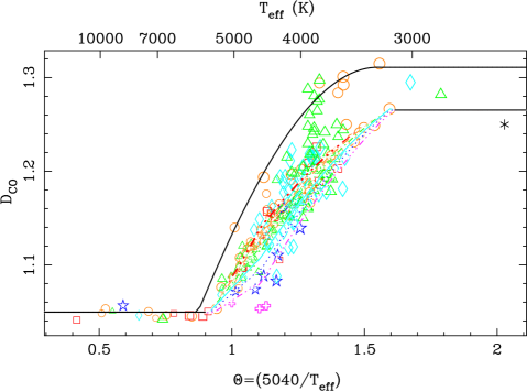
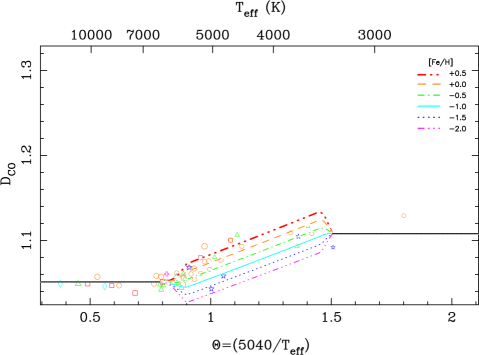
Figure 14: Empirical fitting functions for the D_CO index for giants, including the fit for AGB stars (top panel) and dwarfs (bottom panel), computed as explained in the text. Symbol types and size mean metallicity and gravity, the same than in previous figures. The different lines represent the metallicities [Fe/H]$=+0.5,+0.0,-0.5,-1.0,-1.5,{\rm and}-2.0$, from top to bottom. The reduced scatter for $\theta\leq 0.9$ is due to the absence of CO absorptions for hot stars, as explained in the text.

Fig. 13 shows the behaviour of the D_CO index versus $\theta$ for the stars in the new library. There is a clear dichotomy in the behaviour of stars depending on their gravity. For that reason, we have divided the stellar atmospheric parameter space in two main groups: dwarf stars ($\log g>3.5$ dex) and giant and supergiant stars ($\log g<3.5$ dex). As we explained in § 6.1, there is also a strong dependence of the CO absorption with the effective temperature. That is why we have subdivided each gravity group into different temperature ranges. Independently of their gravity, stars with high effective temperature exhibit no traces of CO absorptions and their index value tends to a constant (D${}_{\rm CO}\simeq 1.05$). On the other hand, due to the lack of very cold stars in both gravity regimes, we have computed a constant value of the index for cold dwarf and giant stars. In short, we have considered three temperature ranges for dwarf stars, while we have considered four different ranges for the giants (see Table 6). The boundaries of these ranges are shown in Fig. 1. In some cases, an overlapping region has been considered. After some experimentation in order to obtain the smoothest fit, we have computed the final index in the intersection region considering a different weight $w$ depending on the case (see Table 6).

Besides the global behaviour described for giant stars, two different trends are found for this type of stars around $\theta=1.3-1.4$ in Fig. 13. After a carefully study of these stars with a higher CO index, we found that they are stars in the asymptotic giant branch (AGB). For that reason, we decided to compute an independent fit for these stars in the range $\theta=1.01-1.56$, shown Fig. 14 (coefficient in Table 6). Since there are no AGB stars for $\theta>1.56$, we simply extrapolate the constant value of the CO index at $\theta=1.56$.

Up to now, we have described the general method to compute fitting functions. However, we have used a slightly different method for cold and warm giant stars. First of all, we have obtained constant fits for hot ($\theta<0.90$) and cold stars ($\theta>1.55$) as explained before. After this, we have generated a set of fake stars with random gravity and metallicity, and effective temperature of $\theta=5040/T_{\mathrm{eff}}=1.60$. Their index values were evaluated from the fitting function computed for cold giant stars. For the associated error of the indices of these fake stars we assumed the mean error of the cold stars. We calculated the local fitting function of cool giants, including these new stars. In this way, we were forcing the fitting function to pass through these stars, i.e., approaching the constant value for cold giants. In a similar way, for the computation of the fitting functions of warm giants, we also created fake stars at $\theta=1.10$ and $\theta=1.13$, and we assigned their index value according to the fitting function for cool stars. A new set of random stars at $\theta=0.92$ was introduced with the constant index value computed from hot stars. Finally, we used these fake stars together with the real stars to obtain the final fit for the warm giants.

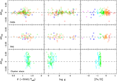
Figure 15: Residuals of the derived fitting functions (observed minus derived) against the three input stellar atmospheric parameters for the stars observed at CAHA (upper panels) and TNG (middle panels). Cluster data from Frogel et al. (2001) and Stephens & Frogel (2004) are presented in lower panels. Codes and relative sizes of the star symbols are explained in Fig. 1 and 13.

We derived the local fitting functions computing a weighted least squares fit to the stars within each parameter range, with weights according to the inverse of the squared uncertainties of the indices for each individual star. Here we considered the nominal errors in the index measurements, using the uncertainties derived in § 4.2 for the library stars, and the individual errors for each cluster quoted by Frogel et al. (2001) and Stephens & Frogel (2004). After the analysis of the residuals, it was necessary to repeat the fitting procedure with the inclusion of additional random uncertainties in some of the stars (see next subsection). The final fitting functions for each stellar parameter range are presented in Table 6. This table includes the functional forms of the fits, the significant coefficients and their corresponding formal errors, the typical index error for the $N$ stars employed in each interval ($\sigma^{2}_{typ}=N/\sum^{N}_{i=1}\sigma^{-1}_{i}$), the unbiased residual variance of the fit ($\sigma^{2}_{\rm std}$) and the determination coefficient ($r^{2}$). Also the intersection regions are indicated and the procedure used for computing the index. We plot in Fig. 14 the fitting functions for giant and dwarf stars as a function of $\theta$ for several metallicities, as well as the simple fit for AGB stars. Fig. 15 shows the final residuals ($\Delta{\rm D_{CO}}={\rm D_{CO\,obs}-D_{CO\,pred}}$) of the new CO index for the different groups of stars used for the computation of the fitting functions (stars observed at CAHA, stars observed at the TNG and cluster stars from previous works) as a function of the atmospheric parameters. As we expected, the residuals for each group of stars do not exhibit any systematic trend.

Users interested in implementing these fitting functions into their population synthesis codes can make use of the FORTRAN subroutine available at the URL address http://www.ucm.es/info/Astrof/ellipt/CO.html.

Table 6: Coefficients and statistical data for the local empirical fitting functions for the D_CO index in each range of stellar parameters.

Hot dwarfs	$0.38<\theta<0.90$	$3.50<\log g<5.50$
exponential fit	N = 28 stars	$\sigma_{\rm typ}=0.00913$
$c_{0}$	$0.0499\pm 0.0011$	$\sigma_{\rm std}=0.00557$
Intersection	Cosine-weighted mean	$0.80<\theta<0.90$
Cool dwarfs	$0.80<\theta<1.50$	$3.50<\log g<5.50$
exponential fit	N = 39 stars	$\sigma_{\rm typ}=0.00748$
$c_{0}$	$-0.0292\pm 0.0330$	$\sigma_{\rm std}=0.01254$
$\theta$	$0.1006\pm 0.0329$	$r^{2}=0.765$
$[{\rm Fe/H}]$	$0.0174\pm 0.0067$
Intersection	Cosine-weighted mean	$1.45<\theta<1.50$
Cold dwarfs	$1.33<\theta<1.80$	$3.50<\log g<5.50$
exponential fit	N = 7 stars	$\sigma_{\rm typ}=0.00960$
$c_{0}$	$0.1025\pm 0.0046$	$\sigma_{\rm std}=0.01195$
Hot giants	$0.42<\theta<0.90$	$-0.40<\log g<3.50$
exponential fit	N = 15 stars	$\sigma_{\rm typ}=0.01954$
$c_{0}$	$0.0459\pm 0.0010$	$\sigma_{\rm std}=0.00398$
Intersection	Cosine-weighted mean	$0.90<\theta<0.93$
Warm giants	$0.90<\theta<1.131$	$0.13\log g<3.5$
exponential fit	N = 63 stars	$\sigma_{\rm typ}=0.00764$
$c_{0}$	$-0.3073\pm 0.0046$	$\sigma_{\rm std}=0.00428$
$\theta$	$0.3876\pm 0.0043$	$r^{2}=0.982$
$[{\rm Fe/H}]$	$-0.1016\pm 0.0042$
$\theta[{\rm Fe/H}]$	$0.1072\pm 0.0039$
$[{\rm Fe/H}]^{2}$	$-0.0023\pm 0.0005$
Intersection	Distance-weighed mean	$1.09<\theta<1.10$
Cool giants	$1.10<\theta<1.60$	$-0.34<\log g<3.41$
exponential fit	N = 167 stars	$\sigma_{\rm typ}=0.01062$
$c_{0}$	$-0.5224\pm 0.0970$	$\sigma_{\rm std}=0.00890$
$\theta$	$0.8257\pm 0.1417$	$r^{2}=0.958$
$[{\rm Fe/H}]$	$0.0674\pm 0.0101$
$\theta[{\rm Fe/H}]$	$-0.0444\pm 0.0065$
$\theta^{2}$	$-0.2200\pm 0.0509$
$[{\rm Fe/H}]^{2}$	$-0.0023\pm 0.0014$
No intersection
Cold giants	$1.55<\theta<2.03$	$-0.07<\log g<3.50$
exponential fit	N = 7 stars	$\sigma_{\rm typ}=0.02156$
$c_{0}$	$0.2397\pm 0.0107$	$\sigma_{\rm std}=0.02698$
AGB stars	$1.01<\theta<1.56$	$-0.11<\log g<1.56$
exponential fit	N = 18 stars	$\sigma_{\rm typ}=0.00612$
$c_{0}$	$-0.8893\pm 0.2198$	$\sigma_{\rm std}=0.00892$
$\theta$	$1.4950\pm 0.3610$	$r^{2}=0.985$
$\theta^{2}$	$-0.4816\pm 0.1461$

6.2.3 Residuals and error analysis

To explore in more detail the reliability of the fitting functions, we computed the unbiased residual standard deviation from the fits, $\sigma_{\rm std}=0.0093$, and the typical error in the measured index, $\sigma_{\rm typ}=0.0025$, for the stars employed in the computation of the global fitting functions derived above.

After the initial fit, we discovered that $\sigma_{\rm std}$ was larger than what should be expected uniquely from index uncertainties (see also the values of $\sigma_{\rm std}$ and $\sigma_{\rm typ}$ for different subgroups of stars in Table 7). Furthermore, a $F$ test of comparison of variances showed that $\sigma_{\rm std}$ was statistically larger than $\sigma_{\rm typ}$, leading to the introduction on an additional residual error ($\sigma_{\rm res}^{2}=\sigma_{\rm std}^{2}-\sigma_{\rm typ}^{2}$). Such residual error could be due to uncertainties in the input stellar atmospheric parameters, not included in the error budget so far. In order to check this, we have computed how errors in the input stellar parameters translate into uncertainties in the predicted D_CO. This depends both on the local functional form of the fitting function and on the atmospheric parameters range (e.g. hot stars have $T_{\mathrm{eff}}$ uncertainties larger than cooler stars). For each star of the sample, we have derived the errors corresponding to the uncertainties in effective temperature ($\sigma_{T_{\mathrm{eff}}}$), gravity ($\sigma_{\log g}$) and metallicity ($\sigma_{\rm[Fe/H]}$). The effect of the uncertainties in the three stellar parameters were finally computed as $\sigma_{\rm par}^{2}=\sigma_{T_{\mathrm{eff}}}^{2}+\sigma_{\log g}^{2}+\sigma_{\rm[Fe/H]}^{2}$. Table 7 presents, summarized for the different stellar groups, all the error estimations already discussed. Finally, in the cases where the residual errors ($\sigma_{\rm res}$) were not explained by the uncertainties in the stellar parameters ($\sigma_{\rm par}$), an extra residual error was added to the original index error. At the end, no iterations were needed for the globular cluster stars and AGB stars, one iteration was required for the giants and two iterations for dwarfs (in any case, the additional error for dwarf stars is lower than the necessary for giants). The uncertainties of the final D_CO fitting functions are listed in Table 8. Note that although in this table $\sigma_{\rm std}$ is still larger than $\sigma_{\rm typ}$ for the four initial subgroups of stars analyzed in Table 7, both standard deviations are statistically comparable using the $F$ test of variances previously mentioned.

Finally, as the purpose of this paper is to predict reliable index values for any combination of input atmospheric parameters, we have also computed the random errors in such predictions. These uncertainties are given in Table 9 for some representative values of input parameters.

Table 7: Uncertainties of the initial D_CO fitting functions for different groups of stars and mean D_CO errors due to uncertainties in the input atmospheric parameters. $N$: number of stars. $\sigma_{\rm std}$: unbiased residual standard deviation for the fit. $\sigma_{\rm typ}$: typical observational D_CO error for the subsample of stars. $\sigma_{\rm res}$: residual error. $\sigma_{T_{\mathrm{eff}}}$ and $\sigma_{\rm[Fe/H]}$: mean D_CO errors due to uncertainties in the input $T_{\mathrm{eff}}$ and [Fe/H] (no error due to uncertainties in the input $\log g$ is computed since the computed fitting functions do not require gravity terms). $\sigma_{\rm par}$: total error due to atmospheric parameters (quadratic sum of the previous errors). $\sigma_{\rm std}$ is not explained by the $\sigma_{\rm typ}$ and $\sigma_{\rm par}$ values for giants and dwarfs, and a residual error has been considered for these group of stars

. $N$ $\sigma_{\rm std}$ $\sigma_{\rm typ}$ $\sigma_{\rm res}$ $\sigma_{T_{\mathrm{eff}}}$ $\sigma_{\rm[Fe/H]}$ $\sigma_{\rm par}$ Field dwarfs 54 0.0059 0.0017 0.0056 0.0010 0.0009 0.0014 Field giants 147 0.0108 0.0023 0.0105 0.0062 0.0019 0.0065 Globular cluster stars 85 0.0276 0.0236 0.0139 0.0010 0.0140 AGB stars 19 0.0115 0.0061 0.0097 0.0000 0.0097 All 305 0.0093 0.0025 0.0075 0.0014 0.0078

Table 8: Uncertainties of the final D_CO fitting functions for different groups of stars and same computed errors than in Table 7.

	$N$	$\sigma_{\rm std}$	$\sigma_{\rm typ}$	$\sigma_{T_{\mathrm{eff}}}$	$\sigma_{\rm[Fe/H]}$	$\sigma_{\rm par}$
Field dwarfs	54	0.0086	0.0078	0.0010	0.0013	0.0017
Field giants	147	0.0123	0.0113	0.0062	0.0014	0.0064
Globular cluster stars	85	0.0252	0.0236	0.0135	0.0009	0.0135
AGB stars	19	0.0115	0.0061	0.0097	0.0000	0.0097
All	305	0.0130	0.0114	0.0074	0.0012	0.0076

Table 9: Absolute errors in the fitting functions predictions for different values of the atmospheric parameters. Input $\log g$ values varying with effective temperature for dwarfs (V), giants (III) and supergiants (I) have been taken from Lang (1991).

			$\sigma[{\rm D_{CO}}]$
$T_{\mathrm{eff}}$	[Fe/H]	V	III	I
6000		0.002	0.001	0.001
5500	$+0.5$	0.010	0.002	0.002
5500	$+0.0$	0.007	0.001	0.001
5500	$-1.0$	0.006	0.001	0.001
5500	$-2.0$	0.011	0.002	0.002
5000	$+0.5$	0.010	0.001	0.001
5000	$+0.0$	0.007	0.001	0.001
5000	$-1.0$	0.005	0.001	0.001
5000	$-2.0$	0.011	0.001	0.001
4500	$+0.5$	0.011	0.004	0.004
4500	$+0.0$	0.008	0.003	0.003
4500	$-1.0$	0.007	0.003	0.003
4500	$-2.0$	0.011	0.006	0.006
4000	$+0.5$	0.014	0.003	0.003
4000	$+0.0$	0.012	0.002	0.002
4000	$-1.0$	0.011	0.003	0.003
4000	$-2.0$	0.014	0.005	0.005
3500	$+0.5$	0.018	0.003	0.007
3500	$+0.0$	0.018	0.003	0.007
3500	$-1.0$	0.018	0.003	0.007
3500	$-2.0$	0.018	0.004	0.007
3000		0.005	0.014	0.014

7 Summary

The aim of this work was to obtain an accurate empirical calibration of the behaviour of the CO feature at 2.3 $\mu$m for individual stars, with the purpose of making it possible to obtain reliable predictions for the CO strength for stellar populations in unresolved systems with a wide range of ages and metallicities. The main results of this work can be summarized as follows:

1. We present a new stellar library in the spectral region around the first CO bandhead at 2.3 $\mu$m. It consists of 220 stars with stellar atmospheric parameters in the range $2485\leq T_{\mathrm{eff}}\leq 13404$ K, $-0.34\leq\log g\leq 5.30$ dex, $-2.63\leq{\rm[Fe/H]}\leq 0.98$ dex.

2. We define a new line-strength index for the first CO bandhead at 2.3 $\mu$m, D_CO, less sensitive to spectral resolution, wavelength calibration, signal-to-noise ratio and flux calibration than previous definitions.

3. We compute empirical fitting functions for the D_CO to parametrize the behaviour of the CO feature as a function of the stellar atmospheric parameters. In this work we quantify, for the first time, the metallicity dependence.

We expect that the work presented in this paper will help researchers to start exploiting in depth the so far poorly-explored and poorly-understood near-IR spectral region centered at 2.3 $\mu$m, since, as we have shown, the strong CO bandhead can be employed to extract useful physical information of composite stellar populations.

Appendix A Stellar library and cluster stars

In Table LABEL:table_stellar_library we list the stars of the stellar library with their spectral type, K magnitude, effective temperature and the associated uncertainty (T_eff and $\sigma[T_{\mathrm{eff}}]$), surface gravity and its uncertainty ($\log g$ and $\sigma[\log g]$), metallicity and its uncertainty ([Fe/H] and $\sigma$[Fe/H]), number of measurements (N), D_CO index and their error $\sigma[{\rm D_{CO}]}$. The stars observed at the TNG are labeled with a ${\dagger}$ in the index measurement.

In Table LABEL:table_cluster_stars we list the cluster stars from Frogel et al. (2001) and Stephens & Frogel (2004) employed in the computation of the empirical fitting functions. We present the derived atmospheric parameters and their associated uncertainties, and the D_CO index and error for each star.

In both tables, AGB stars are labeled with a $\star$ in the name of the star.

Table 11: Stellar library used in the fitting function procedure. Stars marked with a ${\dagger}$ symbol were observed at the TNG. AGB stars are marked with a $\star$ symbol.

Name	Spectral	$K$	$T_{\mathrm{eff}}$	$\sigma[T_{\mathrm{eff}}]$	$\log g$	$\sigma[\log g]$	[Fe/H]	$\sigma$[Fe/H]	N	DCO	$\sigma[{\rm D_{CO}]}$
	Type	(mag)	(K)		(dex)		(dex)
BD+012916	KIIvw	$+6.47$	4150	60.9	0.10	0.18	$-1.99$	0.09	2	1.092	0.010
BD+233130	G0	$+6.95$	5039	75.0	2.42	0.40	$-2.55$	0.15	2	1.058	0.012
BD+442051	M2V	$+4.77$	3696	60.9	5.00	0.18	$-1.50$	0.09	4	1.105†	0.010
G171-010	M6eV	$+5.93$	2799	60.9	5.12	0.18	–	0.09	2	1.129	0.009
HD001326B	M6V	$+5.95$	3344	60.9	5.30	0.18	$-1.40$	0.09	2	1.092	0.009
HD004628	K2V	$+3.68$	4960	75.0	4.60	0.40	$-0.29$	0.15	2	1.080	0.009
HD010307	G2V	$+3.57$	5838	60.9	4.28	0.18	$+0.03$	0.09	2	1.057	0.009
HD013043	G2V	$+5.38$	5695	60.9	3.68	0.18	$+0.10$	0.09	3	1.048	0.009
HD013555	F5V	$+4.12$	6378	60.9	4.01	0.18	$-0.35$	0.09	3	1.048	0.009
HD014221	F4V	$+5.25$	6342	60.9	3.91	0.18	$-0.35$	0.09	3	1.042	0.009
HD014662	F7Ib	$+4.18$	5933	117.6	1.30	0.21	$-0.03$	0.09	3	1.045	0.011
HD015596	G5III-IV	$+3.86$	4755	75.0	2.50	0.40	$-0.70$	0.15	3	1.097	0.011
HD015798	F5V	$+3.47$	6345	60.9	3.85	0.18	$-0.16$	0.09	3	1.057	0.009
HD016901	G0Ib-II	$+3.56$	5345	117.6	0.85	0.21	$+0.00$	0.09	3	1.053	0.010
HD017361	K1.5III	$+2.09$	4600	60.9	2.85	0.18	$-0.02$	0.09	3	1.120	0.011
HD017382	K1V	$+5.61$	5065	75.0	4.50	0.40	$-0.13$	0.15	3	1.066	0.009
HD020619	G0	$+5.46$	5652	60.9	4.48	0.18	$-0.26$	0.09	3	1.054	0.010
HD020893	K3III	$+2.19$	4340	60.9	2.04	0.18	$+0.08$	0.09	3	1.146	0.011
HD021017	K4III	$+2.88$	4410	60.9	2.36	0.18	$+0.00$	0.09	3	1.138	0.011
HD021197	K5V	$+5.12$	4657	117.6	4.59	0.21	$+0.33$	0.10	3	1.100	0.010
HD021910	G8III-IV	$+4.99$	4582	60.9	1.75	0.18	$-0.60$	0.09	3	1.092	0.011
HD023841	K1III	$+3.80$	4279	60.9	1.67	0.21	$-0.95$	0.09	2	1.130	0.012
HD025329	K1Vsb	$+6.20$	4787	75.0	4.58	0.40	$-1.72$	0.15	2	1.058	0.009
HD026297	G5-6IVw	$+6.12$	4316	75.0	1.06	0.40	$-1.67$	0.15	3	1.083	0.011
HD026322	F2IV-V	$+4.48$	7072	60.9	3.49	0.18	$+0.16$	0.09	3	1.043	0.011
HD026846	K3III	$+2.27$	4541	60.9	2.62	0.18	$+0.15$	0.09	2	1.137	0.011
HD027371	K0III	$+1.51$	4271	60.9	3.00	0.18	$+0.34$	0.09	2	1.105	0.011
HD027819	A7V	$+4.41$	8129	60.9	4.00	0.18	$-0.20$	0.09	3	1.047	0.009
HD028305	G9.5III	$+1.42$	4846	60.9	2.68	0.18	$+0.11$	0.09	3	1.106	0.011
HD029139	K5III	$-3.04$	3910	75.0	1.59	0.40	$-0.34$	0.15	3	1.188	0.011
HD030959	M3Svar	$-0.66$	3451	117.6	0.80	0.21	$-0.15$	0.10	3	1.220	0.010
HD031295	A0V	$+4.41$	8991	117.6	4.08	0.21	$-0.89$	0.10	3	1.046	0.009
HD031767	K2II	$+1.34$	4120	60.9	1.78	0.18	$+0.26$	0.09	3	1.164	0.011
HD032147	K3V	$+3.71$	4658	100.0	4.47	0.50	$+0.02$	0.30	3	1.100	0.009
HD035155	S?I	$+2.13$	3600	117.6	0.80	0.21	$-0.72$	0.10	2	1.237	0.012
HD035369	G8III	$+2.06$	4863	75.0	2.50	0.40	$-0.26$	0.15	3	1.097	0.011
HD035601⋆	M1.5Ia	$+1.66$	3550	60.9	0.00	0.18	$+0.00$	0.09	4	1.301†	0.010
HD036003	K5V	$+4.88$	4465	60.9	4.61	0.18	$+0.09$	0.10	3	1.093	0.009
HD036395	M1V	$+4.00$	3590	60.9	4.90	0.21	$-0.45$	0.09	3	1.116	0.009
HD037160	G8III-IV	$+1.80$	4668	75.0	2.46	0.40	$-0.50$	0.15	3	1.105	0.011
HD037536⋆	M2Iabs	$+0.97$	3789	117.6	0.70	0.21	$-0.15$	0.10	3	1.294	0.010
HD037828	K0	$+4.06$	4296	75.0	1.14	0.40	$-1.38$	0.15	3	1.110	0.011
HD037984	K1III	$+2.21$	4404	60.9	2.45	0.18	$-0.26$	0.09	3	1.129	0.011
HD038656	G8III	$+2.24$	4928	60.9	2.52	0.18	$-0.22$	0.09	3	1.085	0.011
HD039364	G8III/IV	$+1.40$	4550	60.9	2.10	0.18	$-0.94$	0.09	3	1.125	0.012
HD039801⋆	M2Iab	$-3.56$	3547	60.9	0.00	0.21	$+0.03$	0.10	3	1.292	0.010
HD040657	K1.5III	$+1.64$	4370	60.9	2.42	0.18	$-0.58$	0.09	3	1.136	0.011
HD041597	G8III	$+2.89$	4700	75.0	2.38	0.40	$-0.54$	0.15	3	1.123	0.011
HD041636	G9III	$+3.97$	4709	60.9	2.50	0.18	$-0.20$	0.09	3	1.116	0.011
HD042474⋆	M2Iabpe…	$+1.85$	3789	117.6	0.70	0.21	$-0.36$	0.10	2	1.277	0.010
HD042543⋆	M1Ia-ab	$+0.80$	3789	117.6	0.00	0.21	$-0.42$	0.10	3	1.298	0.010
HD044007	G5IVw	$+6.97$	4969	75.0	2.26	0.40	$-1.47$	0.15	3	1.071	0.012
HD044889	K0I	$+3.60$	3775	117.6	0.40	0.21	$-0.20$	0.10	4	1.186	0.014
HD045829⋆	K0Iab	$+3.35$	4500	117.6	0.20	0.21	$-0.01$	0.09	2	1.194	0.010
HD047914	K5III	$+1.70$	3962	60.9	1.50	0.18	$+0.05$	0.09	3	1.172	0.011
HD048329	G8Ib	$+0.12$	4150	60.9	0.80	0.21	$+0.20$	0.09	2	1.170	0.012
HD048433	K1III	$+1.93$	4460	100.0	1.88	0.50	$-0.25$	0.30	3	1.120	0.011
HD048565	F8	$+5.80$	5929	60.9	3.59	0.18	$-0.70$	0.09	3	1.048	0.009
HD049161	K4III	$+1.58$	4176	60.9	1.69	0.18	$+0.08$	0.09	3	1.153	0.011
HD049331⋆	M1II	$+0.56$	3600	117.6	0.70	0.21	$-0.03$	0.10	2	1.284	0.010
HD052005	K4Iab	$+2.10$	4117	60.9	0.60	0.18	$-0.20$	0.09	2	1.197	0.011
HD052973	G0Ibvar	$+2.13$	5659	117.6	1.37	0.21	$+0.34$	0.10	3	1.045	0.010
HD054810	K0III	$+2.44$	4697	60.9	2.35	0.18	$-0.30$	0.09	2	1.111	0.011
HD057264	G8III	$+2.75$	4620	60.9	2.72	0.18	$-0.33$	0.09	3	1.116	0.011
HD058207	K0III	$+1.56$	4788	60.9	2.55	0.18	$-0.12$	0.09	3	1.113	0.011
HD058521⋆	M5Ib-IIvar	$-0.68$	3238	60.9	0.00	0.18	$-0.19$	0.09	4	1.315†	0.010
HD060179	A1V	$+1.64$	10286	117.6	4.00	0.21	$+0.98$	0.10	2	1.049	0.009
HD060522	M0III-IIIb	$+0.23$	3899	60.9	1.20	0.18	$+0.12$	0.09	2	1.177	0.015
HD061064	F6III	$+4.21$	6449	60.9	3.21	0.21	$+0.42$	0.09	3	1.048	0.011
HD061603	K5III	$+2.17$	3870	60.9	1.50	0.18	$+0.24$	0.09	3	1.204	0.012
HD061606	K2V	$+4.88$	4833	117.6	4.55	0.21	$+0.07$	0.09	3	1.077	0.009
HD061772	K3III	$+1.33$	3995	60.9	1.47	0.18	$+0.08$	0.09	2	1.203	0.011
HD062345	G8IIIa	$+1.52$	5017	60.9	2.63	0.18	$-0.08$	0.09	3	1.086	0.011
HD062721	K5III	$+1.23$	3954	60.9	1.52	0.18	$-0.22$	0.09	2	1.188	0.011
HD063352	K0III	$+2.87$	4226	60.9	2.20	0.18	$-0.31$	0.09	3	1.153	0.011
HD063791	G0	$+5.42$	4629	75.0	1.76	0.40	$-1.63$	0.15	2	1.074	0.011
HD064332	S?I	$+2.30$	3500	117.6	0.50	0.21	$-0.34$	0.10	2	1.242	0.010
HD065714	G8III	$+3.91$	4840	60.9	1.50	0.18	$+0.27$	0.09	2	1.097	0.012
HD066141	K2III	$+1.44$	4258	60.9	1.90	0.18	$-0.30$	0.09	3	1.145	0.011
HD068284	F8V	$+6.26$	5860	60.9	3.98	0.18	$-0.57$	0.09	3	1.050	0.009
HD069267	K4III	$+0.19$	4043	60.9	1.51	0.18	$-0.12$	0.09	4	1.170†	0.011
HD070272	K5III	$+0.37$	3900	60.9	1.05	0.18	$+0.04$	0.09	3	1.180	0.011
HD072184	K2III	$+3.50$	4624	60.9	2.61	0.18	$+0.12$	0.09	2	1.123	0.013
HD072324	G9III	$+3.97$	4887	60.9	2.13	0.18	$+0.16$	0.09	3	1.099	0.011
HD072905	G1.5Vb	$+4.17$	5864	60.9	4.48	0.18	$-0.04$	0.09	3	1.061	0.010
HD073394	G5IIIw	$+4.95$	4500	60.9	1.10	0.18	$-1.38$	0.09	4	1.088†	0.011
HD073593	G8IV	$+2.96$	4717	60.9	2.25	0.18	$-0.12$	0.09	4	1.120†	0.011
HD074000	F6VI	$+8.39$	6166	60.9	4.19	0.18	$-2.02$	0.09	2	1.061	0.010
HD074395	G2Iab	$+2.85$	5250	117.6	1.30	0.21	$-0.05$	0.09	4	1.076†	0.010
HD074442	K0III	$+1.56$	4657	60.9	2.51	0.18	$-0.06$	0.09	3	1.120	0.011
HD075732	G8V	$+4.01$	5079	75.0	4.48	0.40	$+0.16$	0.15	3	1.076	0.009
HD076813	G9III	$+3.15$	6072	117.6	4.20	0.21	$-0.82$	0.10	4	1.082†	0.010
HD076932	F7-8IV-V	$+4.36$	5866	100.0	3.96	0.50	$-0.93$	0.30	3	1.057	0.009
HD078712	M6SI	$-1.87$	3202	60.9	0.00	0.18	$-0.11$	0.09	4	1.216†	0.010
HD078732	G8II	$+3.20$	4900	117.6	2.00	0.21	$+0.24$	0.10	8	1.108	0.011
HD079211	M0V	$+4.14$	3710	60.9	4.71	0.18	$-0.40$	0.10	3	1.093	0.010
HD079452	G6III	$+3.86$	4829	60.9	2.35	0.18	$-0.84$	0.09	4	1.086†	0.012
HD081192	G7III	$+4.11$	4705	75.0	2.50	0.40	$-0.62$	0.15	4	1.101†	0.011
HD082074	G6IV	$+4.15$	5055	117.6	3.30	0.21	$-0.48$	0.10	2	1.088	0.011
HD082885	G8IV-V	$+3.69$	5488	60.9	4.61	0.18	$+0.00$	0.09	2	1.061	0.009
HD083425	K3III	$+1.58$	4120	60.9	2.00	0.18	$-0.35$	0.09	4	1.170†	0.011
HD083618	K3III	$+0.87$	4231	60.9	1.74	0.18	$-0.08$	0.09	4	1.161†	0.011
HD083632	K2III	$+4.72$	4214	60.9	1.00	0.21	$-1.39$	0.09	4	1.160†	0.011
HD085235	A3IV	$+4.37$	11200	117.6	3.55	0.21	$-0.40$	0.10	3	1.049	0.009
HD085503	K0III	$+1.36$	4472	75.0	2.33	0.40	$+0.23$	0.15	3	1.136	0.011
HD085773	G:w?I	$+7.95$	4463	60.9	0.98	0.18	$-2.17$	0.09	1	1.056	0.014
HD087737	A0Ib	$+3.29$	9625	60.9	1.98	0.21	$-0.04$	0.10	4	1.053†	0.010
HD087822	F4V	$+5.13$	6590	60.9	4.15	0.18	$+0.14$	0.09	4	1.049†	0.009
HD089484	K1IIIb	$-0.81$	4470	60.9	2.35	0.18	$-0.49$	0.09	3	1.119	0.011
HD089822B	A0sp?III	$+3.39$	5538	117.6	2.44	0.21	$+0.51$	0.10	2	1.050	0.010
HD092523	K3III	$+1.55$	4090	60.9	1.96	0.18	$-0.38$	0.09	2	1.163	0.011
HD093487	F8	$+6.76$	5250	60.9	1.80	0.18	$-1.05$	0.09	2	1.068	0.012
HD095578	M0III	$+0.80$	3700	60.9	1.40	0.18	$-0.23$	0.09	2	1.206	0.011
HD095735	M2V	$+3.25$	3551	60.9	4.90	0.21	$-0.20$	0.09	8	1.108†	0.009
HD096360	M?I	$+2.76$	3550	117.6	0.50	0.21	$-0.58$	0.10	4	1.244†	0.012
HD097907	K3III	$+2.43$	4351	60.9	2.07	0.18	$-0.10$	0.09	2	1.162	0.011
HD099648	G8II-III	$+2.83$	4850	117.6	1.90	0.21	$+0.36$	0.10	3	1.097	0.011
HD099998	K4III	$+1.24$	3863	60.9	1.79	0.18	$-0.16$	0.09	4	1.186†	0.011
HD101501	G8Vvar	$+3.58$	5401	60.9	4.60	0.18	$-0.13$	0.09	3	1.054	0.009
HD102224	K0III	$+0.98$	4383	75.0	2.02	0.40	$-0.46$	0.15	2	1.148	0.011
HD102328	K3III	$+2.63$	4390	60.9	2.09	0.18	$+0.35$	0.09	2	1.155	0.011
HD103095	G8Vp	$+4.37$	5025	60.9	4.56	0.18	$-1.36$	0.09	4	1.043†	0.002
HD103877	AmV	$+5.88$	7341	117.6	4.00	0.21	$+0.40$	0.09	1	1.038	0.009
HD104307	K2III	$+3.68$	4451	117.6	2.00	0.21	$-0.01$	0.10	2	1.159	0.012
HD105262	B9	$+6.75$	8542	117.6	1.50	0.21	$-1.37$	0.10	2	1.056	0.010
HD107213	F8Vs	$+5.13$	6298	60.9	4.01	0.18	$+0.36$	0.09	4	1.051†	0.009
HD110014	K2III	$+2.01$	4399	60.9	1.47	0.18	$+0.10$	0.09	3	1.151	0.011
HD111631	M0.5V	$+4.88$	3785	60.9	4.75	0.21	$+0.10$	0.09	4	1.109†	0.011
HD113092	K2III	$+2.11$	4283	60.9	1.95	0.18	$-0.37$	0.09	3	1.148	0.011
HD113285	M8III	$-1.06$	2485	117.6	0.00	0.18	–	–	5	1.250	0.012
HD114038	K1III	$+2.72$	4530	60.9	2.71	0.18	$-0.04$	0.09	4	1.132†	0.011
HD114095	G5	$+5.88$	4650	60.9	2.40	0.18	$-0.70$	0.09	2	1.108	0.011
HD114330	AV1	$+4.30$	9509	117.6	3.80	0.21	$-0.01$	0.10	2	1.057	0.011
HD114946	G6V	$+3.11$	5171	60.9	3.64	0.18	$+0.13$	0.09	3	1.093	0.010
HD114961⋆	M7III	$+1.50$	3012	112.8	0.00	0.18	$-0.81$	0.09	8	1.295†	0.010
HD117176	G5V	$+3.50$	5525	60.9	3.81	0.18	$-0.10$	0.09	2	1.067	0.009
HD117876	G8III	$+3.87$	4782	75.0	2.25	0.40	$-0.50$	0.15	3	1.106	0.012
HD119228	M2III	$+0.33$	3600	60.9	1.60	0.18	$+0.30$	0.09	8	1.203†	0.011
HD119667	K5	$+4.18$	3700	117.6	1.00	0.21	$-0.35$	0.10	4	1.219†	0.011
HD120933	K5III	$-0.00$	3820	60.9	1.52	0.18	$+0.50$	0.09	8	1.226†	0.012
HD121130	M3III	$-0.24$	3672	117.6	1.25	0.21	$-0.24$	0.10	2	1.216	0.012
HD121299	K2III	$+2.85$	4710	60.9	2.64	0.18	$-0.03$	0.09	4	1.125†	0.011
HD122563	F8IV	$+3.73$	4566	75.0	1.12	0.40	$-2.63$	0.15	4	1.053†	0.011
HD122956	G6IV-Vw	$+5.89$	4635	75.0	1.49	0.40	$-1.75$	0.15	2	1.084	0.010
HD123299	A0III	$+3.63$	9894	60.9	2.90	0.21	$+0.12$	0.10	5	1.048	0.011
HD123657	M4III	$-0.23$	3450	60.9	0.85	0.21	$+0.00$	0.09	4	1.231†	0.013
HD124186	K4III	$+3.59$	4347	60.9	2.10	0.18	$+0.24$	0.09	3	1.144	0.011
HD124850	F7IV	$+2.80$	6116	60.9	3.87	0.18	$-0.11$	0.09	3	1.051	0.009
HD124897	K2IIIp	$-2.91$	4361	75.0	1.93	0.40	$-0.53$	0.15	2	1.137	0.013
HD126327	M7.5III	$+1.74$	2819	60.9	0.00	0.18	$-0.58$	0.09	4	1.282†	0.013
HD126681	G3V	$+7.63$	5536	60.9	4.65	0.18	$-1.25$	0.09	2	1.068	0.010
HD126778	K0III	$+5.84$	4847	60.9	2.34	0.21	$-0.62$	0.09	2	1.120	0.011
HD127243	G3IV	$+3.15$	4978	75.0	3.20	0.40	$-0.59$	0.15	3	1.091	0.012
HD130694	K4III	$+1.10$	4040	60.9	1.85	0.18	$-0.34$	0.09	3	1.173	0.011
HD130705	K4II-III	$+3.95$	4336	60.9	2.10	0.18	$+0.41$	0.09	4	1.151†	0.011
HD131430	K2/K3III	$+2.20$	4190	60.9	2.18	0.18	$+0.04$	0.09	4	1.159†	0.011
HD131918	K4III	$+2.09$	3970	60.9	1.49	0.18	$+0.22$	0.09	3	1.173	0.012
HD132345	K3III-IVp	$+3.26$	4374	60.9	1.60	0.18	$+0.23$	0.09	3	1.155	0.013
HD134063	G5III	$+5.47$	4885	60.9	2.34	0.21	$-0.69$	0.09	4	1.109†	0.011
HD135722	G8III	$+1.22$	4847	75.0	2.56	0.40	$-0.44$	0.15	2	1.086	0.011
HD136726	K4III	$+1.93$	4120	60.9	2.03	0.18	$+0.07$	0.09	4	1.190†	0.014
HD137471	M1III	$+1.03$	3422	60.9	1.10	0.18	$+0.07$	0.10	3	1.194	0.010
HD137704	K4III	$+2.11$	4095	60.9	1.97	0.18	$-0.27$	0.09	4	1.166†	0.011
HD137759	K2III	$+0.77$	4498	60.9	2.38	0.18	$+0.05$	0.09	3	1.125	0.012
HD137909	F0p	$+3.45$	8541	117.6	4.25	0.21	$+0.83$	0.10	3	1.047	0.009
HD138481	K5III	$+1.21$	3890	60.9	1.64	0.18	$+0.20$	0.09	4	1.166†	0.018
HD139641	G7.5IIIb	$+3.10$	5030	60.9	3.22	0.18	$-0.55$	0.09	2	1.081	0.011
HD140160	A0p…V	$+5.20$	9164	117.6	3.30	0.21	$-0.25$	0.10	2	1.050	0.011
HD141527	G0Iab:pe	$+4.56$	6816	60.9	0.48	0.18	$-0.50$	0.09	4	1.042	0.014
HD141714	G3.5III	$+2.66$	5230	60.9	3.02	0.18	$-0.29$	0.09	5	1.075	0.012
HD145675	K0V	$+4.71$	5264	75.0	4.66	0.40	$+0.34$	0.15	4	1.080†	0.009
HD146051	M0.5III	$-1.17$	3793	117.6	1.40	0.21	$+0.32$	0.10	2	1.189	0.011
HD147923	M…	$+3.46$	3600	117.6	0.80	0.21	$-0.19$	0.10	4	1.221†	0.011
HD148783	M6III	$+0.29$	3279	112.8	0.20	0.21	$-0.06$	0.09	4	1.249†	0.012
HD148897	G8pII	$+1.96$	4284	117.6	1.15	0.21	$-0.75$	0.09	2	1.116	0.011
HD149009	K5III	$+2.04$	3910	60.9	1.60	0.18	$+0.30$	0.09	3	1.209	0.012
HD149661	K0V	$+3.91$	5168	60.9	4.63	0.18	$+0.04$	0.09	4	1.075†	0.009
HD150012	F5III-IV	$+5.26$	6505	60.9	3.90	0.18	$+0.16$	0.09	3	1.058	0.009
HD150680	F9IV	$+1.28$	5672	60.9	3.74	0.18	$+0.01$	0.09	2	1.055	0.009
HD151203	M3IIIab	$+0.89$	3640	60.9	0.70	0.18	$-0.10$	0.10	3	1.218	0.011
HD154733	K3III	$+2.48$	4279	60.9	2.10	0.18	$+0.00$	0.09	4	1.165†	0.011
HD155763	B6III	$+3.60$	13397	117.6	4.24	0.18	$-0.95$	0.10	2	1.049	0.010
HD156014	M5Ib-II	$-1.99$	3161	112.8	0.00	0.21	$+0.00$	0.09	2	1.267	0.012
HD156026	K5V	$+3.86$	4541	60.9	4.54	0.18	$-0.37$	0.09	2	1.106	0.009
HD156283	K3IIvar	$-0.02$	4460	60.9	2.33	0.18	$+0.18$	0.09	3	1.176	0.011
HD157910	G5III	$+4.39$	5137	60.9	1.83	0.18	$-0.32$	0.09	3	1.077	0.011
HD160933	F9V	$+4.82$	5684	75.0	3.90	0.40	$-0.32$	0.15	2	1.061	0.009
HD161096	K2III	$+0.43$	4543	60.9	2.16	0.18	$+0.08$	0.09	2	1.138	0.016
HD161797	G5IV	$+1.51$	5411	75.0	3.87	0.40	$+0.16$	0.15	3	1.067	0.010
HD161817	A2VI(HB)	$+6.29$	7759	60.9	2.95	0.18	$-0.95$	0.09	2	1.046	0.010
HD163990	M6Svar	$+0.19$	3365	117.6	0.70	0.21	$+0.01$	0.10	3	1.247	0.011
HD163993	G8III	$+1.73$	5028	60.9	2.70	0.18	$+0.03$	0.09	3	1.087	0.012
HD164058	K5III	$-1.16$	3930	60.9	1.26	0.18	$-0.05$	0.09	4	1.189†	0.012
HD164136	F2II	$+2.77$	6799	117.6	2.63	0.21	$-0.30$	0.10	3	1.044	0.011
HD164349	K0.5IIb	$+1.93$	4446	60.9	1.50	0.18	$+0.39$	0.09	4	1.157†	0.011
HD166208	G8III…	$+2.93$	4919	75.0	2.52	0.40	$+0.08$	0.15	3	1.075	0.011
HD167768	G3III	$+3.89$	5235	60.9	1.61	0.21	$-0.68$	0.09	4	1.085†	0.011
HD168322	G8.5IIIb	$+3.93$	4793	60.9	2.00	0.18	$-0.40$	0.09	3	1.111	0.012
HD168720	M1III	$+0.74$	3810	60.9	1.10	0.18	$+0.00$	0.10	4	1.211†	0.012
HD168723	K0III-IV	$+1.05$	4859	75.0	3.13	0.40	$-0.19$	0.15	2	1.099	0.011
HD173819	K0Ibpvar	$+2.15$	4421	117.6	0.00	0.21	$-0.88$	0.10	3	1.121	0.012
HD174638	B7Ve….	$+3.19$	12136	60.9	2.50	0.18	$+0.43$	0.09	3	1.041	0.011
HD175865	M5III	$-1.83$	3520	60.9	0.50	0.18	$+0.14$	0.10	4	1.250†	0.012
HD181096	F6IV:	$+6.47$	6276	75.0	4.09	0.40	$-0.26$	0.15	2	1.047	0.009
HD182835	F2Ib	$+4.01$	7350	721.4	2.15	0.32	$+0.09$	0.29	2	1.050	0.010
HD184499	G0V	$+5.07$	5738	100.0	4.02	0.50	$-0.66$	0.30	4	1.044†	0.009
HD184786	M4.5III	$+0.74$	3467	117.6	0.60	0.21	$-0.04$	0.10	4	1.234†	0.012
HD185144	K0V	$+2.90$	5260	75.0	4.55	0.40	$-0.24$	0.15	4	1.061†	0.009
HD187216	R…	$+6.02$	3500	117.6	0.40	0.21	$-2.48$	0.10	4	1.138†	0.010
HD187921	K0var	$+3.80$	6000	117.6	1.00	0.21	$+0.28$	0.10	3	1.046	0.012
HD188119	G8III	$+1.73$	4915	75.0	2.61	0.40	$-0.32$	0.15	3	1.098	0.012
HD191277	K3III	$+2.72$	4459	60.9	2.71	0.18	$+0.30$	0.09	4	1.131†	0.011
HD195593	F5Iab	$+3.65$	6700	721.4	1.95	0.18	$+0.12$	0.09	3	1.046	0.012
HD199799	M1I	$+1.33$	3400	117.6	0.30	0.21	$-0.24$	0.10	4	1.241†	0.012
HD202447	G0III+…	$+2.34$	6087	60.9	3.24	0.18	$+0.09$	0.09	5	1.085	0.010
HD209369	F5V	$+3.96$	6217	60.9	3.85	0.18	$-0.26$	0.09	2	1.051	0.009
HD216228	K0III	$+1.27$	4768	75.0	2.49	0.40	$+0.01$	0.15	2	1.118	0.011
HD217382	K4III	$+1.49$	4035	60.9	1.24	0.18	$-0.25$	0.09	2	1.182	0.011
HD223047⋆	G5Ib	$+2.47$	4990	117.6	1.50	0.21	$+0.18$	0.10	2	1.140	0.010
HD232078	K4-5III	$+4.19$	4008	60.9	0.30	0.18	$-1.73$	0.09	4	1.139†	0.011

Table 11: continued.

Table 13: Cluster stars used in the fitting function procedure. AGB stars are maked with a $\star$ symbol.

Name	$T_{\mathrm{eff}}$	$\sigma[T_{\mathrm{eff}}]$	$\log g$	$\sigma[\log g]$	[Fe/H]	$\sigma$[Fe/H]	DCO	$\sigma[{\rm D_{CO}]}$
	(K)		(dex)		(dex)
Liller1-6	3612	127.0	$+0.05$	0.11	$-0.61$	0.09	1.250	0.047
Liller1-7	3671	96.0	$+0.07$	0.13	$-0.61$	0.09	1.178	0.043
Liller1-157⋆	4011	121.0	$-0.11$	0.11	$-0.61$	0.09	1.248	0.047
Liller1-158	3671	96.0	$-0.02$	0.11	$-0.61$	0.09	1.245	0.047
Liller1-162	3627	119.0	$+0.29$	0.11	$-0.61$	0.09	1.214	0.045
Liller1-166	3973	118.0	$+0.56$	0.13	$-0.61$	0.09	1.150	0.041
Liller1-299	3150	134.0	$-0.07$	0.11	$-0.61$	0.09	1.255	0.047
M69-1	3830	106.0	$+0.04$	0.10	$-0.78$	0.03	1.215	0.023
M69-II-37	3716	97.0	$+0.09$	0.12	$-0.78$	0.03	1.178	0.022
M69-I-40	3917	113.0	$+0.25$	0.12	$-0.78$	0.03	1.166	0.022
M69-2	3864	109.0	$+0.30$	0.11	$-0.78$	0.03	1.215	0.023
M69-3	3864	109.0	$+0.30$	0.11	$-0.78$	0.03	1.212	0.023
M69-4	3899	112.0	$+0.41$	0.12	$-0.78$	0.03	1.219	0.024
M71-29	3641	108.0	$+0.09$	0.12	$-0.84$	0.06	1.203	0.017
M71-30	3992	120.0	$+0.68$	0.13	$-0.84$	0.06	1.185	0.016
M71-B	3764	100.0	$+0.25$	0.12	$-0.84$	0.06	1.188	0.016
M71-46	4011	121.0	$+0.80$	0.11	$-0.84$	0.06	1.195	0.016
M71-A4	4153	134.0	$+0.79$	0.13	$-0.84$	0.06	1.178	0.016
M71-1=H	3796	103.0	$+0.86$	0.12	$-0.84$	0.06	1.175	0.016
M71-2=I	4565	173.0	$+1.08$	0.11	$-0.84$	0.06	1.149	0.015
M71-3=113	3954	116.0	$+0.83$	0.13	$-0.84$	0.06	1.192	0.016
M71-4=45	4011	121.0	$+0.87$	0.13	$-0.84$	0.06	1.171	0.016
M71-5=64	4153	134.0	$+1.42$	0.10	$-0.84$	0.06	1.159	0.016
M71-6=66	4649	182.0	$+1.39$	0.10	$-0.84$	0.06	1.137	0.015
M71-8=21	4458	162.0	$+1.45$	0.13	$-0.84$	0.06	1.138	0.015
NGC0104-A02	3533	128.0	$+0.08$	0.13	$-0.78$	0.02	1.214	0.035
NGC0104-W12	3780	102.0	$+0.05$	0.10	$-0.78$	0.02	1.225	0.036
NGC0104-A19	3554	128.0	$+0.10$	0.12	$-0.78$	0.02	1.181	0.034
NGC0104-V07	3764	100.0	$+0.21$	0.13	$-0.78$	0.02	1.188	0.034
NGC0104-V06	3864	109.0	$+0.43$	0.12	$-0.78$	0.02	1.172	0.033
NGC0104-L168	3882	110.0	$+0.43$	0.12	$-0.78$	0.02	1.215	0.035
NGC0104-5529	3973	118.0	$+0.64$	0.13	$-0.78$	0.02	1.205	0.035
NGC0104-2426	4070	126.0	$+0.93$	0.12	$-0.78$	0.02	1.170	0.033
NGC0104-1505	4070	126.0	$+0.96$	0.12	$-0.78$	0.02	1.184	0.034
NGC0104-4418	4091	128.0	$+0.95$	0.11	$-0.78$	0.02	1.188	0.034
NGC0104-1510	4153	134.0	$+1.01$	0.14	$-0.78$	0.02	1.168	0.033
NGC0104-2416	4219	140.0	$+1.33$	0.15	$-0.78$	0.02	1.177	0.034
NGC0104-6408	4383	155.0	$+1.44$	0.14	$-0.78$	0.02	1.163	0.033
NGC0288-A96	4070	126.0	$+0.50$	0.10	$-1.14$	0.03	1.144	0.016
NGC0288-A78	4132	132.0	$+0.67$	0.11	$-1.14$	0.03	1.148	0.016
NGC0288-C20	4153	134.0	$+0.71$	0.11	$-1.14$	0.03	1.118	0.015
NGC0288-A77	4219	140.0	$+0.83$	0.10	$-1.14$	0.03	1.135	0.016
NGC0288-A245	4433	160.0	$+1.10$	0.12	$-1.14$	0.03	1.124	0.015
NGC0362-III11	4011	121.0	$+0.37$	0.10	$-1.09$	0.03	1.162	0.035
NGC0362-IV100	4091	128.0	$+0.50$	0.10	$-1.09$	0.03	1.145	0.034
NGC0362-III63	4031	123.0	$+0.52$	0.10	$-1.09$	0.03	1.169	0.036
NGC0362-III44	4091	128.0	$+0.66$	0.10	$-1.09$	0.03	1.119	0.033
NGC0362-III70	4310	148.0	$+0.75$	0.10	$-1.09$	0.03	1.088	0.031
NGC5927-100⋆	3847	107.0	$+0.01$	0.11	$-0.64$	0.01	1.246	0.046
NGC5927-799	3847	107.0	$+0.38$	0.12	$-0.64$	0.01	1.243	0.045
NGC5927-627	3864	109.0	$+0.51$	0.11	$-0.64$	0.01	1.203	0.043
NGC5927-532	3992	120.0	$+0.80$	0.12	$-0.64$	0.01	1.167	0.041
NGC5927-622	4175	136.0	$+1.00$	0.15	$-0.64$	0.01	1.152	0.040
NGC5927-536	4310	148.0	$+1.27$	0.15	$-0.64$	0.01	1.191	0.042
NGC6388-1	3954	116.0	$-0.34$	0.13	$-0.74$	0.18	1.238	0.038
NGC6388-3	3899	112.0	$-0.05$	0.11	$-0.74$	0.18	1.230	0.038
NGC6388-4	3701	96.0	$+0.09$	0.13	$-0.74$	0.18	1.204	0.037
NGC6440-KF-1	3847	107.0	$+0.41$	0.13	$-0.62$	0.10	1.179	0.018
NGC6440-KF-2	3813	105.0	$+0.46$	0.11	$-0.62$	0.10	1.210	0.018
NGC6440-KF-3	3716	97.0	$+0.47$	0.12	$-0.62$	0.10	1.196	0.018
NGC6440-KF-4	3686	94.0	$+0.50$	0.12	$-0.62$	0.10	1.193	0.018
NGC6440-KF-5	3864	109.0	$+0.53$	0.11	$-0.62$	0.10	1.239	0.019
NGC6440-KF-6	3747	99.0	$+0.57$	0.12	$-0.62$	0.10	1.188	0.018
NGC6440-KF-8	3747	99.0	$+0.67$	0.11	$-0.62$	0.10	1.196	0.018
NGC6440-KF-7	3796	103.0	$+0.67$	0.12	$-0.62$	0.10	1.201	0.018
NGC6528-7	3864	109.0	$+0.30$	0.11	$-0.61$	0.08	1.220	0.029
NGC6528-11	3732	98.0	$+0.05$	0.11	$-0.61$	0.08	1.242	0.030
NGC6528-22⋆	3813	105.0	$+0.37$	0.12	$-0.61$	0.08	1.275	0.031
NGC6528-6⋆	3917	113.0	$+0.41$	0.12	$-0.61$	0.08	1.248	0.030
NGC6553-20	3780	102.0	$-0.16$	0.12	$-0.60$	0.04	1.209	0.034
NGC6553-19	3551	138.0	$-0.02$	0.10	$-0.60$	0.04	1.227	0.035
NGC6553-25	3747	99.0	$+0.14$	0.14	$-0.60$	0.04	1.229	0.036
NGC6553-16⋆	3917	113.0	$+0.27$	0.11	$-0.60$	0.04	1.288	0.038
NGC6553-26⋆	3847	107.0	$+0.32$	0.13	$-0.60$	0.04	1.281	0.038
NGC6553-14⋆	3813	105.0	$+0.38$	0.12	$-0.60$	0.04	1.265	0.037
NGC6553-2	3656	105.0	$+0.42$	0.12	$-0.60$	0.04	1.192	0.034
NGC6624-KF-1	3917	113.0	$+0.40$	0.11	$-0.70$	0.03	1.230	0.034
NGC6624-KF-2	3917	113.0	$+0.53$	0.13	$-0.70$	0.03	1.160	0.030
NGC6624-KF-3	3917	113.0	$+0.54$	0.13	$-0.70$	0.03	1.162	0.030
NGC6624-KF-4	3899	112.0	$+0.82$	0.14	$-0.70$	0.03	1.218	0.033
NGC6624-KF-5	4070	126.0	$+0.96$	0.15	$-0.70$	0.03	1.197	0.032
NGC6712-LM5$\star$	4111	130.0	$+0.55$	0.10	$-0.94$	0.03	1.223	0.024
NGC6712-LCO1	4132	132.0	$+0.58$	0.11	$-0.94$	0.03	1.211	0.023
NGC6712-LCO3	4219	140.0	$+0.61$	0.10	$-0.94$	0.03	1.188	0.023
NGC6712-LM8	4111	130.0	$+0.71$	0.11	$-0.94$	0.03	1.157	0.022
NGC6712-LM10	4264	144.0	$+0.72$	0.10	$-0.94$	0.03	1.194	0.023
NGC6712-B66	4196	138.0	$+0.85$	0.12	$-0.94$	0.03	1.195	0.023
Terzan2-1	4241	142.0	$+0.40$	0.10	$-0.65$	0.14	1.158	0.034
Terzan2-2	3973	118.0	$+0.41$	0.11	$-0.65$	0.14	1.205	0.037
Terzan2-3⋆	3899	112.0	$+0.43$	0.12	$-0.65$	0.14	1.260	0.040
Terzan2-4	4175	136.0	$+0.44$	0.11	$-0.65$	0.14	1.215	0.037
Terzan2-5	3936	115.0	$+0.56$	0.12	$-0.65$	0.14	1.200	0.037
Terzan2-7	4111	130.0	$+0.61$	0.10	$-0.65$	0.14	1.199	0.037
Terzan2-8	4132	132.0	$+0.62$	0.10	$-0.65$	0.14	1.151	0.034

Table 13: continued.