Evidence for primordial mass segregation in globular clusters

Abstract

We have studied the dissolution of initially mass segregated and unsegregated star clusters due to two-body relaxation in external tidal fields, using Aarseth’s collisional $N$-body code NBODY4 on GRAPE6 special-purpose computers. When extrapolating results of initially not mass segregated models to globular clusters, we obtain a correlation between the time until destruction and the slope of the mass function, in the sense that globular clusters which are closer to dissolution are more strongly depleted in low-mass stars. This correlation fits observed mass functions of most globular clusters. The mass functions of several globular clusters are however more strongly depleted in low-mass stars than suggested by these models. Such strongly depleted mass functions can be explained if globular clusters started initially mass segregated. Primordial mass segregation also explains the correlation between the slope of the stellar mass function and the cluster concentration which was recently discovered by De Marchi et al. (2007). In this case, it is possible that all globular clusters started with a mass function similar to that seen in young open clusters in the present-day universe, at least for stars below $m=0.8$ M_⊙. This argues for a near universality of the mass function for different star formation environments and metallicities in the range $-2<\mbox{[Fe/H]}<0$. We finally describe a novel algorithm which can initialise stationary mass segregated clusters with arbitrary density profile and amount of mass segregation.

1 Introduction

In recent years, stellar mass functions have been obtained for an increasing number of globular clusters by deep HST and VLT measurements (see DeMarchi et al. 2007 and references therein). These observations have shown that there is a considerable spread in the present-day mass functions of individual clusters, and that a number of star clusters are strongly depleted in low-mass stars. If one expresses the mass function of a cluster as a power-law by $dN/dm\sim m^{-\alpha}$, where $N$ is the number of stars per unit mass $m$, the observed slopes range from between $\alpha=1.9$ to $\alpha=-0.9$ for stars with masses in the range $0.3<m<0.8$ M_⊙. For clusters where information from different radii is available, the data point to a global decrease of the number of low-mass stars in the clusters, rather than a local effect due to mass segregation.

The depletion of low-mass stars can in principle be understood by mass segregation and the preferential loss of low-mass stars as a result of the dynamical evolution of star clusters. Indeed, using direct $N$-body simulations, Baumgardt & Makino (2003) found a correlation between the observed and expected slopes for the then available sample of star clusters. However, for a number of clusters, the difference between theoretical and expected slope is far too large to be explained just by observational uncertainties.

This is emphasised by De Marchi et al. (2007), who found a correlation between the mass function slope $\alpha$ and the concentration parameter $c=\log_{10}(r_{t}/r_{c})$ for globular clusters, where $r_{t}$ and $r_{c}$ are the tidal and core radius of the cluster as determined from the projected light density profile. The correlation found by De Marchi et al. (2007) is in the sense that clusters with small values of $c$ are depleted in low-mass stars, while clusters with large values of $c$ have mass functions still rising towards small masses. Since simulations show that mass segregation and the preferential loss of low-mass stars should only happen after a cluster has gone into core-collapse, and since core-collapse is connected to the shrinkage of the core size $r_{c}$, the observed correlation is the exact opposite of the theoretically expected one.

One possible interpretation of this finding would be that star clusters that formed more concentrated have a bottom-heavy IMF, which would be a challenge to star formation theories and dispose the universality of the IMF. However this conclusion needs to be tested by taking into account the stellar-dynamical evolution of the clusters.

In the present paper we compare the observational results with theoretical predictions by Baumgardt & Makino (2003) (BM03), who have performed a large parameter study of initially not mass segregated multi-mass clusters evolving under the combined influence of relaxation, stellar evolution and an external tidal field. We also report results of new simulations of multi-mass star clusters which start initially mass segregated. Initial mass segregation is expected to occur in star clusters as a result of star formation feedback in dense gas clouds (Murray & Lin, 1996) and due to competitive gas accretion and mutual mergers between protostars (Bonnell & Bate, 2002). Numerous studies have also found observational evidence for it in young star clusters of the Milky Way and the Magellanic Clouds (Bonnell & Davies, 1998; Gouliermis et al., 2004; Chen et al., 2007), so that it is certainly possible that globular clusters started mass segregated.

The paper is organised as follows: In §2 we compare the results of simulations of non-mass-segregated clusters done by Baumgardt & Makino (2003) with the observed mass function slopes of globular clusters. In §3 we describe the numerical simulations of star clusters with primordial mass segregation and in §4 we compare the results of these runs with the observations. We briefly summarize in §5.

2 Models without primordial mass segregation

BM03 performed a large set of $N$-body simulations of multi-mass star clusters moving in external tidal fields and evolving under the combined influence of two-body relaxation, an external tidal field and stellar evolution. All models contained between 8.192 to 131.072 stars and started with a canonical mass function that consisted of two power-laws with slope $\alpha=1.3$ for stars between 0.08 and 0.5 M_⊙ and slope $\alpha=2.3$ for more massive stars (Kroupa, 2001). The clusters moved on circular or eccentric orbits through an isothermal galaxy with circular velocity $V_{C}=220$ km/sec. BM03 obtained the following expression for the lifetime $T_{Diss}$ of a star cluster:

$$\frac{T_{Diss}}{\mbox{[Myr]}}\;=\;\beta\;\left(\frac{N}{ln(\gamma\,N)}\right)^{x}\;\frac{R_{G}}{\mbox{[kpc]}}\;\left(\frac{V_{G}}{220\;\mbox{km/sec}}\right)^{-1}(1-\epsilon)\,\,,$$ (1)

where $N$ is the number of cluster stars, $\gamma=0.02$ a constant in the Coulomb logarithm and $R_{G}$ and $\epsilon$ the apocenter distance and eccentricity of the cluster orbit, respectively. The constants $\beta$ and $x$ were found to depend on the density profile. For King $W_{0}=7$ models, $x$ and $\beta$ are given by $x=0.82$ and $\beta=1.03$. BM03 found that mass is lost more or less linearly with time from a star cluster, except for the mass lost due to stellar evolution, which decreases the initial mass by about 30% within the first Gyr. The mass left at a time $T<T_{Diss}$ can therefore be approximated by

$$M(T)=0.70\,M_{0}\,(1-T/T_{Diss})\;\;\;\;\;.$$ (2)

BM03 also found that, while the clusters are dissolving, mass segregation causes massive stars to sink into the cluster center and low-mass stars to move to the outer parts, where they are easily removed by the tidal field, so that the global mass function of stars gets depleted in low-mass stars. By fitting power-law mass functions $dN/dm\sim m^{-\alpha}$ to the mass function of stars with $m<0.5$ M_⊙, BM03 derived the following expression for the change in the slope of the mass function:

$$\alpha=1.3-1.51\left(\frac{T}{T_{Diss}}\right)^{2}+1.69\left(\frac{T}{T_{Diss}}\right)^{3}-1.50\left(\frac{T}{T_{Diss}}\right)^{4}\;.$$ (3)

They found that this expression gave a good fit to the change of the mass function for a wide range of initial cluster orbits and cluster masses. Since observed mass function slopes of the clusters in De Marchi et al. (2007) are determined mainly from stars with masses $0.3$ M${}_{\odot}<m<0.8$ M_⊙, we have re-analysed the data by BM03 and find that the following formula fits the change of the mass function in this range:

$$\alpha=1.74-0.34\frac{T}{T_{Diss}}+4.52\left(\frac{T}{T_{Diss}}\right)^{2}-7.59\left(\frac{T}{T_{Diss}}\right)^{3}+5.86\left(\frac{T}{T_{Diss}}\right)^{4}\;.$$ (4)

The runs by BM03 also indicated that the mass-to-light ratio drops as a cluster evolves and loses preferentially low-mass stars which do not contribute much to the overall cluster light. The results of BM03 (their Fig. 14) can be fitted by the relation

$$M/L=1.5-0.5\frac{T}{T_{Diss}}\;.$$ (5)

Using the above equations 1, 2 and 5, we can calculate the initial mass of individual globular clusters, provided their orbits and present-day luminosities are known. One way to do this is to first guess two initial masses $M_{Low}$ and $M_{Up}$ which lead to too small and too large present-day masses, and then iterate to the correct initial mass by interval-halving. Once the initial masses and dissolution times are known, the expected present-day mass function slopes of low-mass stars can be calculated from eq. 4. Table 1 and Fig. 1 compare our predictions with the observed slopes from De Marchi et al. (2007). We have taken the pericenter and apocenter distances from Dinescu et al. (1999), except for NGC 6496 for which a circular orbit at the current Galactocentric distance was assumed since its proper motion is not known. The integrated luminosities were taken from Harris (1996). We assumed an age of $T=12$ Gyr for the Galactic globular cluster system.

Table 1: Observed and theoretical mass function slopes for globular clusters. The first three columns give the name, observed global mass function slope $\alpha$ and cluster concentration $c$, taken from De Marchi et al. (2007). The next columns give the absolute luminosity, pericenter and apocenter distance taken from Harris (1996) and Dinescu et al. (1999). The final columns come from our fit using eqs. 1, 2, 4 and 5, and give the lifetime, initial and present-day cluster mass and expected mass function slope for stars in the range $0.3<m<0.8$ M_⊙ of initially unsegregated clusters.

Cluster	$\alpha_{Obs}$	$c$	$M_{V}$	$R_{Peri}$	$R_{Apo}$	$T_{Diss}$	$M_{Cini}$	$M_{C}$	$\alpha_{Th}$
				[kpc]	[kpc]	[Gyr]	[$M_{\odot}$]	[$M_{\odot}$]
NGC 104	1.2	2.03	-9.42	5.2	7.3	85.7	$1.1\cdot 10^{6}$	$7.0\cdot 10^{5}$	1.73
NGC 288	0.0	0.96	-6.74	1.7	11.2	17.4	$2.2\cdot 10^{5}$	$4.8\cdot 10^{4}$	0.98
NGC 2298	-0.5	1.28	-6.30	2.3	15.7	17.7	$1.4\cdot 10^{5}$	$3.2\cdot 10^{4}$	1.02
Pal 5	0.4	0.70	-5.17	7.0	19.0	14.3	$1.0\cdot 10^{5}$	$1.0\cdot 10^{4}$	0.35
NGC 5139	1.2	1.61	-10.29	1.2	6.2	55.7	$2.7\cdot 10^{6}$	$1.5\cdot 10^{6}$	1.69
NGC 5272	1.3	1.84	-8.93	5.5	13.4	82.6	$7.2\cdot 10^{5}$	$4.5\cdot 10^{5}$	1.73
NGC 6121	1.0	1.59	-7.20	0.6	5.9	14.3	$7.0\cdot 10^{5}$	$6.7\cdot 10^{4}$	0.30
NGC 6218	-0.1	1.29	-7.32	2.6	5.3	21.3	$2.6\cdot 10^{5}$	$8.7\cdot 10^{4}$	1.33
NGC 6254	1.1	1.40	-7.48	3.4	4.9	24.3	$2.7\cdot 10^{5}$	$1.0\cdot 10^{5}$	1.43
NGC 6341	1.5	1.81	-8.20	1.4	9.9	25.2	$5.3\cdot 10^{5}$	$2.0\cdot 10^{5}$	1.42
NGC 6352	0.6	1.10	-6.48	3.3	3.3	16.4	$1.8\cdot 10^{5}$	$3.7\cdot 10^{4}$	0.94
NGC 6397	1.4	2.50	-6.63	3.1	6.3	18.8	$1.6\cdot 10^{5}$	$4.5\cdot 10^{4}$	1.19
NGC 64961	0.7	0.70	-7.23	4.3	4.3	23.1	$2.2\cdot 10^{5}$	$8.2\cdot 10^{4}$	1.40
NGC 6656	1.4	1.31	-8.50	2.9	9.3	41.2	$5.5\cdot 10^{5}$	$2.9\cdot 10^{5}$	1.64
NGC 6712	-0.9	0.90	-7.50	0.9	6.2	16.4	$5.1\cdot 10^{5}$	$9.4\cdot 10^{4}$	0.84
NGC 6752	1.6	2.50	-7.73	4.8	5.6	31.8	$2.9\cdot 10^{5}$	$1.4\cdot 10^{5}$	1.57
NGC 6809	1.3	0.76	-7.55	1.9	5.8	20.9	$3.3\cdot 10^{5}$	$1.1\cdot 10^{5}$	1.30
NGC 6838	-0.2	1.15	-5.60	4.5	6.7	16.2	$8.4\cdot 10^{4}$	$1.7\cdot 10^{4}$	0.90
NGC 7078	1.9	2.50	-9.17	5.4	10.3	86.0	$9.0\cdot 10^{5}$	$5.6\cdot 10^{5}$	1.73
NGC 7099	1.4	2.50	-7.43	3.0	6.9	24.6	$2.6\cdot 10^{5}$	$1.0\cdot 10^{5}$	1.44

¹We assumed a circular orbit for NGC 6496 at its current Galactocentric distance since the proper motion of this cluster is not known.

Figure 1: Observed mass function slope vs. lifetime remaining to dissolution as determined from the current mass of each cluster and eqs. 1 and 2. The errorbar in the lower left corner shows typical uncertainties of the observed slopes which are around 0.2. The observed mass function slopes show a clear correlation in the sense that clusters closer to dissolution are on average more strongly depleted in low-mass stars. The dashed line shows the expected mass function slope for clusters without primordial mass segregation, determined from the models of Baumgardt & Makino (2003) (eq. 4). It provides a good fit for most clusters, however a number of clusters close to dissolution are much more strongly depleted in low-mass stars.

Fig. 1 compares the predicted mass function slopes with the observations. It can be seen that all clusters with remaining lifetimes larger than $T=20$ Gyr have nearly identical slopes with $\alpha\approx 1.5$. This value is close to the expected slope for stars with $0.3<m<0.8$ M_⊙ drawn from a canonical IMF, $\alpha=1.7$. Globular clusters have therefore started with a mass function slope at the low mass end which is similar to that seen for open clusters in the present-day universe. Fig. 1 also shows that, in agreement with the theoretical results from the $N$-body simulations, the mass functions of clusters close to dissolution become depleted in low-mass stars. While some clusters lie close to the predictions from the models of BM03 (dashed line), a number of clusters are significantly stronger depleted in low-mass stars. In the $N$-body models, slopes with $\alpha<0$ are hardly reached since the clusters first have to go into core-collapse to become mass segregated and then dissolve before reaching a strong enough depletion of low-mass stars. Hence, these clusters cannot be explained with the type of initial conditions used by Baumgardt & Makino (2003), i.e. clusters that form in dynamical equilibrium, filling their tidal radii and start without primordial mass segregation. In addition, the correlation of mass function slope and cluster concentration noted by De Marchi et al. (2007) is difficult to understand with non-mass-segregated clusters (see Fig. 3, left panel).

As explained in the Introduction, several lines of evidence indicate that star clusters form mass segregated, in which case the depletion of low-mass stars could happen much quicker than in the models by Baumgardt & Makino (2003). This offers a possible way how to explain the observations. We will therefore explore the influence of primordial mass segregation in the next sections.

3 $N$-body models of mass segregated clusters

In order to understand if primordial mass segregation helps reconciling the discrepancy between observations and simulations, we calculated a number of models starting with primordial mass segregation. All runs were performed with the collisional $N$-body code NBODY4 (Aarseth, 1999) on the GRAPE6 computers of Bonn University. The modeled clusters contained between $10.000$ to $90.000$ stars initially. Since these numbers are rather small compared to particle numbers in globular clusters, we decided to omit stellar evolution and start all runs with a power-law mass function with slope $\alpha=1.3$ between lower and upper mass limits of $m=0.1$ and $m=1.2$ M_⊙. This should capture the essential physics of the collisional evolution of globular clusters. In order to account for the break in slope of the canonical IMF at 0.5 M_⊙, we assume that for stars more massive than 0.5 M_⊙, only a fraction $0.5M_{\odot}/m$ of stars are main-sequence stars while the other are compact remnants which are not taken into account when mass function slopes are determined. All clusters started from King $W_{0}=3.0$ density profiles and moved on circular orbits through an isothermal Galaxy. In order to study the influence of the initial cluster size, we calculated two sets of models, one in which the tidal radius of the external tidal field, $r_{J}$, was equal to the tidal radius of the King model, $r_{J}/r_{t}=1$, and one set of tidally underfilling models with $r_{J}/r_{t}=3$. The algorithm for creating mass segregated clusters in virial equilibrium is described in the Appendix. In our models, we studied the evolution of unsegregated clusters and clusters in which the mass and energy arrays are completely ordered before stars are assigned positions and velocities. These models therefore show the maximum influence mass segregation can have and realistic clusters should lie between the two extremes covered by our simulations. Table 2 summarises the runs performed.

Table 2: Details of the $N$-body models. The second column gives the initial number of cluster stars, the third column whether or not primordial mass segregation was present. The fourth column gives the tidal filling factor $r_{J}/r_{t}$ and the last two columns give the dissolution time, defined to be the time when 99% of the mass is lost, and the core collapse time, expressed in $N$-body units (Heggie & Hut, 2002).

Nr.	N	PMS	$r_{J}/r_{t}$	$T_{Diss}$	$T_{CC}$
				[NBODY]	[NBODY]
1	10.0000	Yes	1.0	1326	564
2	10.0000	No	1.0	1380	728
3	30.0000	Yes	1.0	2534	1550
4	30.0000	No	1.0	2703	1686
5	90.0000	Yes	1.0	5097	3582
6	90.0000	No	1.0	5666	3976
7	10.0000	Yes	3.0	6522	778
8	10.0000	No	3.0	6160	886
9	30.0000	Yes	3.0	11850	1970
10	30.0000	No	3.0	11960	2130

4 Results for mass segregated clusters

Fig. 2 depicts the evolution of the mass function of initially mass segregated clusters starting from various initial conditions and compares it with the evolution of non-segregated clusters and observations of Galactic globular clusters. Final mass functions were determined from a fit to the distribution of stars in the mass range $0.3M_{\odot}<m<0.8M_{\odot}$, similar to the mass range for which observed mass functions are determined for most star clusters. It can be seen that in tidally underfilling models (upper panels with $r_{J}/r_{t}=3.0$), the evolution does not depend much on whether the cluster initially starts mass segregated or not. This is probably due to the short core collapse times of strongly concentrated clusters compared with their dissolution times (see Table 2). Since the starting condition has largely been erased by the time a cluster goes into core collapse, and since the pre-core collapse evolution typically lasts only about 20% of the total lifetime for these models, the starting condition should not strongly influence the overall evolution. The lower panels in Fig. 2 depict the evolution of tidally filling clusters with $r_{J}/r_{t}=1.0$. While non-segregated clusters still evolve close to the prediction of Baumgardt & Makino (2003) (dotted lines), the evolution of mass segregated clusters is now markedly different: Since in mass segregated clusters, low-mass stars start close to the tidal radius, they are being depleted right from the start of the simulations, leading to final mass functions much more strongly depleted in low-mass stars. The amount of depletion is strong enough to explain most observed mass functions. Hence, the range of slopes seen for Galactic globular clusters can, at least in principle, be explained if some started mass segregated while others didn’t, or all of them started mass segregated but with a range of tidal filling factors. We also note that the expulsion of residual gas within the first Myr can enhance the depletion of low-mass stars if the clusters start mass segregated (Marks, Kroupa & Baumgardt, 2008).

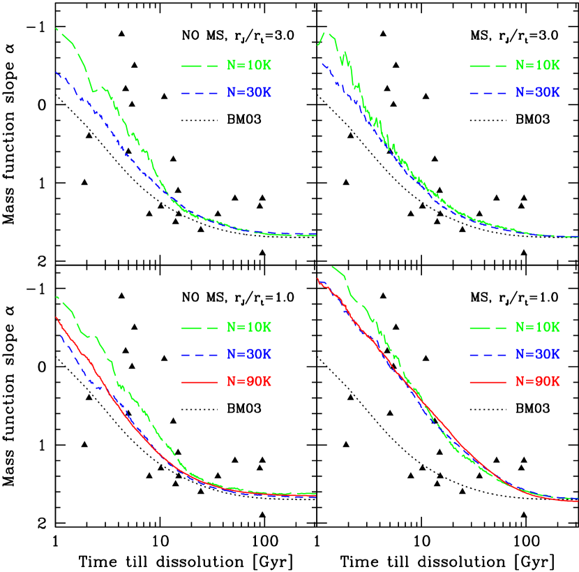
Figure 2: Same as Fig. 1, but now for mass segregated and not mass segregated clusters. The upper panels depict the evolution of tidally underfilling clusters with $r_{J}/r_{t}=3.0$, the lower panels that of clusters with $r_{J}/r_{t}=1.0$. The left panels depict the evolution of non-segregated clusters, the right panels that of mass segregated clusters. Mass segregated clusters in strong tidal fields lose low-mass stars right from the start of the simulations, leading to more strongly depleted mass functions by the time the clusters are close to dissolution. This can explain the mass function slopes of strongly depleted globular clusters. In most cases, mass functions evolve nearly independently of the initial number of stars.

Fig. 3 finally depicts the evolution of star clusters in the concentration vs. mass function slope plane. In order to determine the concentration, King models were fitted to the surface density distribution of stars with masses in the range $0.6\leq m\leq 0.8$ M_⊙ and the concentration $c$ was chosen from the King model which gave the best fit to the simulated clusters. The restriction to stars in the mass range $0.6\leq m\leq 0.8$ M_⊙ was done since in globular clusters these would be the stars which create most of the cluster light. As can be seen, the cluster concentration first increases in all models as the clusters go into core collapse and then decreases again in post-collapse due to core expansion driven by binaries in the cluster centre. In post-collapse, all models reach a stable value of $c=1.6$ nearly independent of the initial concentration. Clusters also move upward in Fig. 3 as the mass function becomes depleted in low-mass stars. For initially non-segregated clusters (left panel), core collapse is fast enough that they are always in post-collapse by the time they have become strongly depleted in low-mass stars. Especially concentrated clusters hardly lose any stars in the pre-collapse phase. Since our clusters started from already very low-concentration, King $W_{0}=3.0$ models, it seems impossible to delay core collapse much further by doing simulations of even lower concentration models. Hence, as was already noted by De Marchi et al. (2007), one cannot explain low-concentration clusters which are strongly depleted in low-mass stars by non-segregated models assuming that the IMF of stars is universal.

The right panel of Fig. 3 depicts the evolution of initially mass segregated clusters. For tidally underfilling clusters with $r_{J}/r_{t}=3.0$, the evolution is virtually indistinguishable from the evolution of non-segregated clusters with $r_{J}/r_{t}=3.0$. Clusters with $r_{J}/r_{t}=1.0$ on the other hand lose low-mass stars much quicker and go into core collapse only after their mass function has become significantly depleted in low-mass stars. Primordial mass segregation would therefore also provide an explanation for low concentration globular clusters which are strongly depleted in low-mass stars.

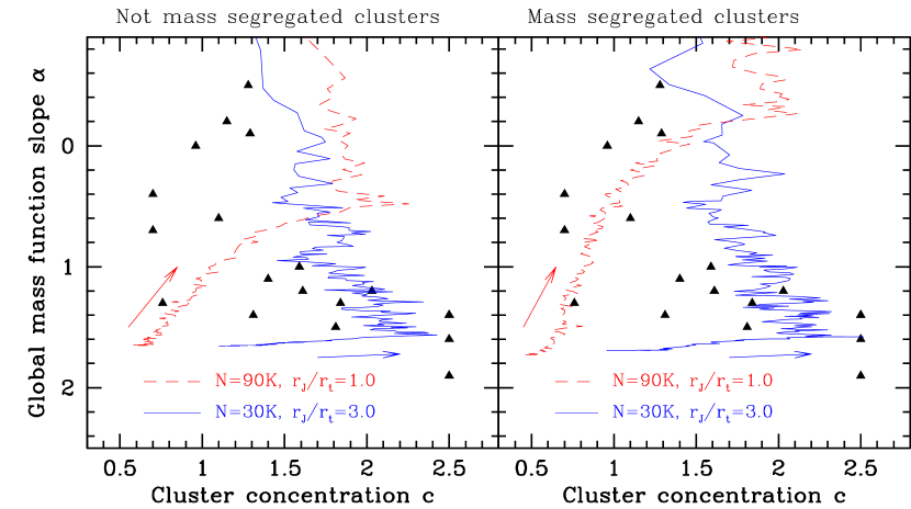
Figure 3: Evolution of initially non-mass-segregated (left panel) and mass segregated (right panel) clusters in the concentration vs. mass function slope plane. The arrows mark the direction in which the clusters are evolving. The cluster concentration first increases as the clusters go into core collapse and then decreases again in post-collapse evolution. Initially not mass segregated clusters are always in post-collapse by the time they have become significantly depleted in low-mass stars, making it impossible to explain clusters with both low concentration and strongly depleted mass functions. In contrast, clusters filling their tidal boundary ($r_{J}/r_{t}=1.0$) and with primordial mass segregation become significantly depleted in low-mass stars before going into core collapse.

5 Conclusions

We have followed the dynamical evolution of star clusters in tidal fields starting with and without primordial mass segregation. We find that clusters with primordial mass segregation lose their low-mass stars more rapidly than non-segregated ones if being immersed in a strong external tidal field, due to the fact that low-mass stars start their lifes in the outer cluster parts where they can easily be removed by the tidal field. For clusters in weaker tidal fields, primordial mass segregation makes only a small difference to the cluster evolution since strong mass loss starts only after core collapse, by which time cluster evolution has largely erased the initial conditions. For all studied models, the absolute values of the core collapse time and the lifetime decrease by no more than 10% due to the introduction of primordial mass segregation. The difference could be larger for simulations which also include the effects of stellar evolution, although e.g. Ardi, Baumgardt & Mineshige (2008) found only a slight increase in core-collapse time for mass segregated clusters compared to non-segregated ones.

Our simulations show that primordial mass segregation is a way to explain the strong depletion of low-mass stars seen in some globular clusters as well as the correlation between mass function slope and cluster concentration recently found by De Marchi et al. (2007). Given the strong observational evidence for primordial mass segregation in young star clusters, we conclude that at least some, but possibly all, globular clusters started mass segregated. The range of mass function slopes seen for Galactic globular clusters can then be explained if they started with a range of tidal filling factors but all of them had the same initial mass function slope. Also, the clusters in the De Marchi et al. (2007) sample span a range of metallicities $-2.2<\mbox{[Fe/H]}<-0.6$ and formed at high redshifts, while current ($z\sim 0$) star formation with $\mbox{[Fe/H]}\approx 0.0$ produces an indistinguishable IMF. Our results therefore indicate that the initial mass function of low-mass stars has been more or less universal for a large range of star formation environments, redshifts and cluster metallicities.

The effect of primordial mass segregation on the mass function is enhanced if residual gas removal is taken into account, since due to the sudden drop of the cluster potential as a result of gas expulsion, stars at large radii are preferentially lost from star clusters. Gas expulsion also naturally leads to tidally filling clusters. The influence of this effect together with the effect of unresolved binaries on the observed mass functions is discussed in Marks, Kroupa & Baumgardt (2008). Their study shows that the effect of gas expulsion depends on several parameters, like the amount of gas removed (i.e. the star-formation efficiency), the timescale over which gas expulsion happens and how strongly the proto-globular cluster is immersed in an external tidal field (see the grid of models run by Baumgardt & Kroupa 2007). Due to their high masses, embedded globular clusters must have started with ratios of half-mass radius to tidal radius, $r_{h}/r_{t}$, significantly smaller than 0.1. Also, the crossing time of a $r_{h}=1$ pc, $10^{6}$ M_⊙ proto-globular cluster is only 20.000 yr, while e.g. Baumgardt, Kroupa & Parmentier (2008) found that gas expulsion from globular clusters should take several $10^{5}$ to $10^{6}$ yr. Hence the primordial gas was probably removed adiabatically (i.e. on a timescale much longer than the crossing time of the cluster) from globular clusters. As can be seen from fig. 3 of Marks et al. (2008), clusters with $r_{h}/r_{t}$ values smaller than 0.06 and adiabatic gas removal mostly preserve their IMF or receive only small changes to it, even when ending up with low concentrations. Hence, while primordial gas expulsion might contribute to the change in the IMF, gas expulsion alone is not likely to explain strongly depleted mass functions in globular clusters.

Primordial binaries also influence measured mass function slopes because a fraction of low-mass stars is hidden in binaries with more massive primaries and because cluster evolution, especially the evolution after core-collapse, is different if primordial binaries are present. The influence of hidden low-mass stars on the mass function slope is also discussed in Marks, Kroupa & Baumgardt (2008). The influence of primordial binaries on cluster evolution is less clear since for example the simulations by Fregeau & Rasio (2007) show that clusters with primordial binaries reach concentrations around $c\approx 2$ in the post-collapse phase, which is close to the values found here for clusters without primordial binaries. Also, in mass segregated, multi-mass clusters, primordial binaries are likely to have a smaller effect on the evolution, since the cluster evolution is driven by only few active binaries. If massive stars start their life in the core, they quickly form binaries and the later cluster evolution becomes indistinguishable from clusters with primordial binaries.

It therefore remains to be seen how results change for models which self-consistently include the effects of gas expulsion, two-body relaxation and primordial binaries. We plan to carry out such studies in the future.

We finally suggest a new method for setting-up mass segregated clusters, which has the advantage that it always creates clusters which are in virial equilibrium since the mass density profile is not changed due to the introduction of mass segregation. It is also flexible and can work with any given mass density profile, initial mass function of stars and can be combined with any scheme for setting up mass segregation.

Appendix A Creation of mass segregated clusters

Primordial mass segregation is introduced by first creating a set of $N^{\prime}$ positions and velocities for an unsegregated cluster, distributed according to the desired mass density profile (King profiles in our case). This set is then ordered according to the specific energy of each star (potential plus kinetic), putting lowest-energy stars first. In a second step, we create an array of $N$ masses, distributed according to the desired mass function, and sort this array in descending order. Here $N$ is the number of stars in the final cluster. We then calculate the cumulative mass function $M_{Cum}[i]=\sum_{i^{\prime}=1}^{i}M[i^{\prime}]$ of all stars in the mass array and divide $M_{Cum}[i]$ by the total mass, so that $M_{Cum}[i]$ runs from 0 to 1. We finally pick a position and velocity for each star $i$ in the mass array by randomly choosing an entry between $N^{\prime}M_{Cum}[i-1]$ and $N^{\prime}M_{Cum}[i]$ from the energy array. In order to make sure that there is at least one entry from which to choose a position and velocity, the energy array has to contain at least $N^{\prime}=N<\!m\!>/m_{Low}$ stars, where $<\!m\!>$ and $m_{Low}$ are the average mass of stars and the mass of the lowest mass star in the mass array.

The above method has the advantage that it creates clusters which are in virial equilibrium since the mass density profile is not changed due to the introduction of mass segregation. In contrast to a method which sorts stars according to radii rather than energies, it also creates clusters in which each individual mass group is in virial equilibrium (see discussion in Ardi, Baumgardt & Mineshige (2008)). The above method is also fast since the most time consuming part of the calculation, the sorting of the energies, is only of order $O(N^{\prime}logN^{\prime})$. By introducing only partial ordering in the mass or energy array one can create clusters with a smaller amount of mass segregation. Fig. 4 shows as an example the evolution of Lagrangian radii for a Plummer model with a Salpeter like mass function going from $0.1M_{\odot}$ to $15M_{\odot}$ which is 100% mass sorted initially As can be seen, not only are the Lagrangian radii of all stars stable, but also those of individual mass groups. We finally note that a different method for creating mass segregated clusters, which uses mean interparticle potentials, has recently also been suggested by Šubr, Kroupa & Baumgardt (2008). Compared to their method, the method suggested here has the advantage that it is more straightforward to create clusters with a desired density profile and that our clusters are always in virial equilibrium.

Figure 4: Evolution of Lagrangian radii for a completely mass-segregated Plummer model as a function of time (which is expressed in units of initial crossing time). Shown is the evolution of Lag. radii containing (from bottom to top) 1%, 5%, 10%, 20%, 50% and 90% of the total mass of each component. As can be seen, not only are the Lagrangian radii for all stars stable, but also those of each individual sub-component.

References

- Aarseth (1999) Aarseth, S. J. 1999, PASP, 111, 1333
- Ardi, Baumgardt & Mineshige (2008) Ardi E., Baumgardt H., Mineshige S., 2008, ApJ in press, arXiv:0804.2299
- Baumgardt & Makino (2003) Baumgardt, H., Makino, J. 2003, MNRAS, 340, 227 (BM03)
- Baumgardt & Kroupa (2007) Baumgardt, H., Kroupa, P. 2007, MNRAS, 380, 1589
- Baumgardt, Kroupa & Parmentier (2008) Baumgardt, H., Kroupa, P., Parmentier, G. 2008, MNRAS, 384, 1231
- Bonnell & Davies (1998) Bonnell, I.A.,& Davies, M.B. 1998, MNRAS, 295, 691
- Bonnell & Bate (2002) Bonnell, I.A., & Bate, M.R. 2002, MNRAS, 336, 659
- Chen et al. (2007) Chen, L., De Grijs, R., Zhao, J. L. 2007, AJ, 134, 1368
- De Marchi et al. (2007) De Marchi, G., Paresce, F., Pulone, L. 2007, ApJ, 656, L65
- Dinescu et al. (1999) Dinescu D. I., Girard T. M., van Altena W. F. 1999, AJ, 117, 1792
- Fregeau & Rasio (2007) Fregeau, J. M., Rasio, F. A. 2007, ApJ, 658, 1047
- Gouliermis et al. (2004) Gouliermis D., Keller S.C., Kontizas M., Kontizas E., Bellas-Velidis I., 2004, A&A, 416, 137
- Harris (1996) Harris W. E. 1996, AJ, 112, 1487
- Heggie & Hut (2002) Heggie, D.C., Hut, P., 2002, The Gravitational Million-Body Problem, Cambridge University Press, p. 8
- Kroupa (2001) Kroupa, P. 2001, MNRAS, 322, 231
- Marks, Kroupa & Baumgardt (2008) Marks M., Kroupa P., Baumgardt H., 2008, MNRAS in press, arXiv:0803.0543
- Murray & Lin (1996) Murray, S.D. & Lin, D.N.C. 1996, ApJ, 467, 728
- Šubr, Kroupa & Baumgardt (2008) Šubr, L., Kroupa, P., Baumgardt, H., MNRAS, 385, 1673