Theory of Helimagnons in Itinerant Quantum Systems IV:
Transport in the Weak-Disorder Regime

Abstract

We apply a recent quasiparticle model for the electronic properties of metallic helimagnets to calculate the transport properties of three-dimensional systems in the helically ordered phase. We focus on the ballistic regime $\tau^{2}T\epsilon_{\text{F}}>>1$ at weak disorder (large elastic mean-free time $\tau$) or intermediate temperature. In this regime, we find a leading temperature dependence of the electrical conductivity proportional to $T$. This is much stronger than either the Fermi-liquid contribution ($T^{2}$) or the contribution from helimagnon scattering in the clean limit ($T^{5/2}$). It is reminiscent of the behavior of non-magnetic two-dimensional metals, but the sign of the effect is opposite to that in the non-magnetic case. Experimental consequences of this result are discussed.

I Introduction

The electrical transport properties of metals have given rise to various surprises over the last thirty years. Within a nearly-free electron model with quenched or static disorder, and to lowest order in the impurity concentration, the Boltzmann equation is exact and yields the familiar Drude expression for the electrical conductivity,

$$\sigma_{0}=ne^{2}\tau/m_{e}\ ,$$ (1)

with $n$ the electron number density, $e$ the electron charge, $m_{\text{e}}$ the effective electron mass, and $\tau$ the elastic mean-free time between collisions, which is weakly temperature dependent. Corrections to this result, in an expansion in the small parameter $1/\epsilon_{\text{F}}\tau$, with $\epsilon_{\text{F}}$ the Fermi energy, turned out to be very interesting. To analyze them, one needs to distinguish, in the thermodynamic limit, between the diffusive regime at strong disorder or low temperature, $T\tau\ll 1$, and the ballistic regime at weak disorder or intermediate temperature, $T\tau\gg 1$. (The latter regime should not be confused with ballistic transport in mesoscopic systems, where the mean-free path is large compared to the system size.) In three-dimensional (3D) simple metals in the diffusive regime, the leading correction is nonanalytic in the temperature $T$, Gorkov et al. (1979); not

$$\delta\sigma_{\text{WL}}\propto\sigma_{0}\,\frac{(T\tau)^{1/2}}{(\epsilon_{\text{F}}\tau)^{2}}\quad\text{(3D, diffusive)}\quad.$$ (2a)

The sign of this effect is positive, which reflects a negative $$T$$-independent contribution that is non-universal (i.e., depends on an ultraviolet cutoff). The effect thus is localizing, i.e., it decreases the conductivity compared to the Drude value. In two-dimensional (2D) systems the effect is even more dramatic, Abrahams et al. (1979)

$$\delta\sigma_{\text{WL}}\propto\sigma_{0}\,\frac{\ln(T\tau)}{\epsilon_{\text{F}}\tau}\quad\text{(2D, diffusive)}\quad.$$ (2b)

These results have been reviewed in Ref. Lee and Ramakrishnan, 1985. The logarithmic divergency in 2D perturbation theory signals a breakdown of transport theory, and the behavior at $T=0$ is insulating, albeit very weakly so. These effects in non-interacting electron systems in general, and the logarithmic temperature dependence in 2D in particular, are known as “weak localization”. They can be understood in terms of constructive interference in the electron-impurity scattering process,Bergmann (1984) or in terms of the exchange of certain soft or massless diffusive modes (either “Cooperons”, or “diffusons”) between electrons.

Taking into account the screened Coulomb interaction between electrons leads to additional effects, and considerably enhances the complexity of the calculations. In the absence of quenched disorder, Fermi-liquid theory accurately describes the behavior and leads to a conductivity given by the Drude formula

$$\sigma_{C}=ne^{2}\tau_{C}/m_{\text{e}},$$ (3a)

with a Coulomb scattering rate proportional to $$T^{2}$$,Schmid (1974)

$$1/\tau_{C}=\frac{\pi^{3}}{8}\,\frac{T^{2}}{\epsilon_{\text{F}}}\ .$$ (3b)

In the presence of both disorder and a Coulomb interaction, and in the diffusive regime, the leading corrections in the diffusive regime are qualitatively the same as those shown in Eqs. (2).Altshuler et al. (1980); Altshuler and Aronov (1984) However, the physics behind the effects is different, and this is reflected in, e.g., the sensitivity of the results to an external magnetic field. These effects are often referred to as “Altshuler-Aronov effects”. In the ballistic regime, $T\tau\gg 1$, the same problem has been analyzed for 2D systems by Zala et al. Zala et al. (2001) They found

$$\delta\sigma_{\text{AA}}\propto\sigma_{0}\,T/\epsilon_{\text{F}}\quad\text{(2D, ballistic)}\quad.$$ (4a)

The sign of the correction depends on the interaction strength, but generically it is localizing, as it is in the diffusive regime. More generally, the conductivity correction can be written

$$\delta\sigma_{\text{AA}}/\sigma_{0}=\frac{1}{\epsilon_{\text{F}}\tau}\,f(T\tau),$$ (4b)

with $f(x\rightarrow 0)\propto\ln x$, and $f(x\rightarrow\infty)\propto x$ in 2D. The crossover between the two limits was also determined in Ref. Zala et al., 2001, and a physical interpretation in terms of scattering by Friedel oscillations was given.

The most appropriate interpretation of $\delta\sigma_{\text{AA}}$ is as the result of a correction to the clean Fermi-liquid relaxation rate $1/\tau_{C}$. In the ballistic regime, this correction is small compared to $1/\tau_{C}$ by a factor of $1/T\tau\ll 1$. Adding this correction to $1/\tau_{C}$ and $1/\tau$ according to Matthiesen’s rule leads, in the regime where $1/\tau_{C}\ll 1/\tau$, to Eq. (4a). Another possible interpretation of $\delta\sigma_{\text{AA}}$ is as an interaction-induced temperature dependent correction to $\sigma_{0}$. In the Coulomb case, $\delta\sigma_{\text{AA}}$ is small compared to both $\sigma_{C}$ and $\sigma_{0}$, but we will see later that this is not necessarily true if the correction is mediated by a different interaction.

A general explanation of the physics behind these nonanalytic temperature dependencies is as follows. If there are massless excitations that couple to the relevant electronic degrees of freedom, then the lack of a mass in the excitation propagator will lead to integrals that are singular in the infrared, and these singularities are protected by a nonzero temperature $T>0$ (or frequency in the zero-temperature limit), which leads to a nonanalytic dependence on $T$. Notice that the massless excitation does not have to be of non-electronic origin: with a proper classification of modes they can themselves be electronic in nature without leading to double counting. For instance, in the case of the weak-localization singularities the relevant soft mode is either the Cooperon, or the diffuson, which are electronic particle-hole excitations that are distinct from, but couple to, the current mode whose correlations determine the conductivity. An example of a non-electronic mode that couples to the current is an acoustic phonon in the presence of an electron-phonon coupling. Since the latter is relatively weak, this leads to a $T$-dependence that is far subleading to the Fermi-liquid $T^{2}$ contribution, namely, the well-known Bloch-Grüneisen $T^{5}$ law.

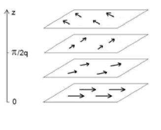
Figure 1: Schematic magnetization pattern in a helimagnet.

In this paper we consider the exchange of a more exotic soft mode, namely, the helimagnon excitation in metallic helimagnets. Helimagnets, the best known examples of which are MnSi and FeGe, form a class of magnetic materials with a preferred axis in spin space, characterized by a vector ${\bm{q}}$. The magnetization displays ferromagnetic order in any plane perpendicular to ${\bm{q}}$, but the direction of the magnetization rotates as one moves along the ${\bm{q}}$-axis, forming a spiral with wavelength $2\pi/q$, where $q\equiv|{\bm{q}}|$ is the pitch wave number, see Fig. 1. A theory of the ordered phase has been developed in Refs. Belitz et al., 2006a, b, which we will refer to as paper I and paper II, respectively. The magnetic order splits the conduction band, as in the case of a ferromagnet, with a Stoner splitting $\lambda$ that is proportional to the local magnetization. The Goldstone mode related to the broken symmetry in spin space, the helimagnon, has been studied in paper II. As one might expect, the helimagnon has an anisotropic frequency-momentum relation,

$$\omega_{0}({\bm{k}})=\sqrt{c_{z}k_{z}^{2}+c_{\perp}{\bm{k}}_{\perp}^{4}}.$$ (5a)

The helimagnon is thus ferromagnon-like in the direction perpendicular to $${\bm{q}} {\bm{q}} {\bm{q}} z {\bm{k}}_{\perp} {\bm{k}} {\bm{q}} c_{z} c_{\perp}$$, and antiferromagnon-like in the direction along . Here and in what follows we take the pitch vector to point in the -direction, and is the component of the wave vector perpendicular to . The elastic constants and are given by

$$c_{z} = \gamma_{z}\,\lambda^{2}\,q^{2}/k_{\text{F}}^{4},$$ (5b)

$$c_{\perp} = \gamma_{\perp}\,\lambda^{2}/k_{\text{F}}^{4}.$$ (5c)

where $k_{\text{F}}$ is the Fermi wave number,F_f and $\gamma_{z}$ and $\gamma_{\perp}$ are numbers. For the model considered in papers I and II their values are

$$\gamma_{z}=1/36\quad,\quad\gamma_{\perp}=1/96.$$ (6)

We will adopt these values for the purposes of this paper.

For later reference we note that the helical magnetization structure is a result of the spin-orbit interaction, which is weak compared to the exchange interaction. Consequently, the pitch wave number $q$, which is proportional to the spin-orbit interaction, is small compared to the Fermi wave number, $q/k_{\text{F}}\ll 1$.

The metallic helimagnet MnSi in particular is a very well-studied material with many unusual properties that have been reported and discussed in detail in Refs. Ishikawa et al., 1976; Pfleiderer et al., 1997, 2001 and papers I and II, among others. Here we focus on the electrical conductivity in the ordered phase, which displays helical order with a helix wavelength $2\pi/q\approx 180\,\AA$ below a critical temperature $T_{\text{c}}\approx 30\,{\text{K}}$ at ambient pressure. Transport measurements in the ordered phase have so far shown no significant deviations from Fermi-liquid $T^{2}$-behavior. Consistent with this, a theoretical investigation of the clean limit in paper II showed that the leading effects of the helimagnons is a $T^{5/2}$ correction to the Fermi-liquid behavior. Our motivation for investigating disorder corrections to the clean behavior is two-fold: First, the residual resistance of the cleanest MnSi samples puts them in the ballistic regime, and simple considerations suggest very interesting behavior in that regime. Second, MnSi shows very unusual transport behavior in the paramagnetic phase, namely, a $T^{3/2}$-behavior of the resistivity over almost three decades in temperature.Pfleiderer et al. (2001) The origin of this is not understood, but it is natural to speculate that remnants of the helical order, which are observed in the same region, have something to do with it. It thus is prudent to first do a comprehensive study of effects of the helical order in the ordered phase, where conditions are more clearly defined.

At a technical level, adding quenched disorder to the formalism used in papers I and II would be hard. We thus employ an effective model that was developed in Ref. pap, a, which we will refer to as paper III. Equations in papers I-III will be referenced in the format (I.x.y), etc.pap (b)

This paper is organized as follows. In Sec. II we list our most important results for the convenience of readers who may not be interested in the technical details. In Sec. III we set up a transport theory based on the effective model, using the Kubo formalism. We first check, and demonstrate the efficiency of, the model by reproducing the clean-limit results of paper II in Sec.  III.1, and then proceed with the calculation in the ballistic limit in Sec. III.2. We discuss our results in Sec. IV. Some general points pertinent to transport theory are made in Appendix A, and several calculational details are relegated to additional appendices.

II Results

Since the details of the transport calculation for helimagnets are quite technical, we first list our most pertinent results without any derivation.

In the helically ordered phase, the conductivity tensor is diagonal, but not isotropic. Taking the pitch vector ${\bm{q}}$ in $z$-direction, its nonzero elements are $\sigma_{zz}\equiv\sigma_{\text{L}}$, and $\sigma_{xx}=\sigma_{yy}\equiv\sigma_{\perp}$. We find the leading correction to the conductivity in the ballistic regime in 3D to be proportional to $\tau T$. For a cubic crystal structure, as is the case for MnSi, we have

$$\delta\sigma_{\text{L}}=3\delta\sigma_{\perp}=-\sigma_{0}\,\frac{\pi\nu^{2}\sqrt{6}}{8}\,\left(\frac{\epsilon_{\text{F}}}{\lambda}\right)^{2}\,\left(\frac{q}{k_{\text{F}}}\right)^{3}\,\frac{T}{\epsilon_{\text{F}}}\ ,$$ (7)

where $\nu$ is a parameter measuring deviations from a spherical Fermi surface, see Eq. (11) below, and the prefactor of the $T$-dependence is accurate to lowest order in the small parameter $q/k_{\text{F}}$.

This result is valid in a window of intermediate temperatures. For asymptotically low temperatures, one finds diffusive, rather than ballistic, transport behavior, and for higher temperatures the ballistic behavior crosses over to either the Fermi-liquid behavior or the clean helimagnet conductivity, which is proportional to $1/T^{5/2}$, see paper II. For realistic parameter values (for known helimagnets), the temperature window is

$$T_{\text{ball}}\ll T\ll T_{\text{ball}}\,(\epsilon_{\text{F}}\tau)\,(q/k_{\text{F}})^{3}\,(\epsilon_{\text{F}}/\lambda)^{3},$$ (8)

where $T_{\text{ball}}\propto\lambda/(\epsilon_{\text{F}}\tau)^{2}$ is the lower limit of the ballistic regime. In this regime the dominant temperature dependence of the conductivity is given by Eq. (7), and the conductivity is

$$\sigma_{\text{L},\perp}=\sigma_{0}+\delta\sigma_{\text{L},\perp}(T).$$ (9)

Notice that the sign of the correction is opposite to the Coulomb case, Eq. (4a). That is, the effect of the helimagnon exchange is antilocalizing. We will derive these results in Sec. III and discuss them in Sec. IV.

III Electrical conductivity of itinerant helimagnets

We now set up a standard technical formalism for transport theory in the context of the effective model for metallic helimagnets that was given in Eq. (III.2.19). The electrical conductivity tensor $\sigma_{ij}$ can be expressed in terms of an equilibrium current-current correlation function by means of the Kubo formula

$$\sigma_{ij}(i\Omega)=\frac{i}{i\Omega}\,\left[\pi_{ij}(i\Omega)-\pi_{ij}(i\Omega=0)\right]\ ,$$ (10a)

where

$$\pi_{ij}(i\Omega) = -e^{2}T\sum_{i\omega_{1},i\omega_{2}}\frac{1}{V}\sum_{{\bm{p}}_{1},{\bm{p}}_{\,2}}j_{i}({\bm{p}}_{1})\,j_{j}({\bm{p}}_{\,2})\sum_{{\sigma_{1}},{\sigma_{2}}}$$ (10b)

$$\hskip-30.0pt\times\bigl{\langle}{\bar{\eta}}_{\sigma_{1}}({\bm{p}}_{1},i\omega_{1})\,\eta_{\sigma_{1}}({\bm{p}}_{1},i\omega_{1}+i\Omega)\,$$

$$\hskip 0.0pt\times{\bar{\eta}}_{\sigma_{2}}({\bm{p}}_{\,2},i\omega_{2})\,\eta_{\sigma_{2}}({\bm{p}}_{\,2},i\omega_{2}-i\Omega)\bigr{\rangle}.$$

is the current-current susceptibility or polarization function, with ${\bar{\eta}}$ and $\eta$ the fermionic fields. $\left\langle\ldots\right\rangle$ denotes an average with respect to the action in Eq. (III.2.19). $i\omega\equiv i\omega_{n}=i2\pi T(n+1/2)$ and $i\Omega\equiv i\Omega_{n}=i2\pi Tn$ $(n=\text{integer})$ are fermionic and bosonic Matsubara frequencies, respectively, and for simplicity we suppress the index $n$. $j({\bm{p}})=\partial\epsilon_{\bm{p}}/\partial{\bm{p}}$ is the current vertex, and for the electronic energy-momentum relation we use an expression appropriate for a cubic crystal structure,

$$\epsilon_{\bm{p}}=\frac{{\bm{p}}^{\,2}}{2m_{\text{e}}}+\frac{\nu}{2m_{\text{e}}k_{\text{F}}^{2}}\,\left(p_{x}^{\,2}p_{y}^{\,2}+p_{y}^{\,2}p_{z}^{\,2}+p_{z}^{\,2}p_{x}^{\,2}\right)+O(p^{\,6}),$$ (11)

with $m_{\text{e}}$ the electronic effective mass, and $\nu=O(1)$ a dimensionless coupling constant that measures deviations from a spherical Fermi surface.

The conductivity as written above is actually the transport coefficient for the quasiparticles defined in paper III, which are described by the fermionic fields ${\bar{\eta}}$ and $\eta$. The physical conductivity is given in terms of the electron fields ${\bar{\psi}}$ and $\psi$, which are related to the quasiparticle fields by the transformation given in Eqs. (III.2.9). However, we will work to lowest order in the small parameter $q/k_{\text{F}}$, and to this accuracy the quasiparticle conductivity is the same as the physical conductivity, as can readily be seen from Eqs. (III.2.9).

The four-point fermionic correlation function in Eq. (10b) is conveniently expressed in terms of Green functions ${\cal G}$ and a vector vertex function ${\bm{\Gamma}}$ with components $\Gamma^{\,i}$,

Figure 2: Graphic representation of the polarization function. The directed solid lines denote Green functions.

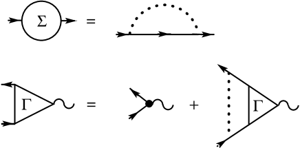
Figure 3: Conserving approximation for the self energy and the vertex function. The dotted line denotes the effective potential.

$$\pi_{ij}(i\Omega) = -e^{2}T\sum_{i\omega}\frac{1}{V}\sum_{\sigma}ij_{\,i}({\bm{p}})\,{\cal G}_{\sigma}({\bm{p}},i\omega)\,{\cal G}_{\sigma}({\bm{p}},i\omega-i\Omega)$$ (12)

$$\hskip 50.0pt\times\Gamma^{j}_{\sigma}({\bm{p}}\,;i\omega,i\omega-i\Omega),$$

see Fig. 2. This expression is valid if the Green function $\langle\eta_{\sigma_{1}}({\bm{p}}_{1},i\omega_{1})\,{\bar{\eta}}_{\sigma_{2}}({\bm{p}}_{\,2},i\omega_{2})\rangle$ is diagonal in both momentum and spin. For our effective model this is the case (whereas it was not the case in paper II), and ${\cal G}$ is expressed in terms of the self energy $\Sigma$ by means of the usual Dyson equation

$${\cal G}_{\sigma}({\bm{p}},i\omega)=\frac{1}{G_{0,\sigma}^{-1}({\bm{p}},i\omega)-\Sigma_{\sigma}({\bm{p}},i\omega)}\ .$$ (13)

Here $G_{0}$ is the bare Green function, which is given by Eq. (III.2.10c). Equations (12, 13) just shift the problem into the determination of the self energy $\Sigma$ and the vertex function ${\bm{\Gamma}}$. In order to evaluate the Kubo formula, it is most convenient to separately treat the cases with and without quenched disorder, respectively.

III.1 Clean limit

We first use the formalism developed so far to re-derive some of the results of paper II for the conductivity of helimagnets in the absence of any elastic scattering. This serves both as a check, and as a demonstration of how much simpler it is to evaluate the Kubo formula within the quasiparticle model compared to the model used in paper II. The calculation presented here is just a slight generalization of what is presented in Appendix A, which serves to discuss the extent to which the approximations used are controlled.

III.1.1 Conserving approximation for the conductivity

It is well known that, in clean systems, care must be taken to treat the self energy $\Sigma$, which enters the Green function $\cal{G}$, and the vertex function ${\bm{\Gamma}}$ consistently in a conserving approximation.Baym and Kadanoff (1961); Kadanoff and Baym (1962) The simplest consistent approximation, which is equivalent to the Boltzmann equation, is to treat the self energy in a self-consistent Born approximation, and the vertex function in a ladder approximation. These are graphically represented in Fig. 3. Analytically we have integral equations

$$\Sigma_{\sigma}({\bm{p}},i\omega) = -T\sum_{i\Omega}\frac{1}{V}\sum_{{\bm{k}}}V({\bm{k}};{\bm{p}}-{\bm{k}},{\bm{p}};i\Omega)$$ (14a)

$$\times{\cal G}_{\sigma}({\bm{p}}-{\bm{k}},i\omega-i\Omega),$$

for the self energy, and

$${\bm{\Gamma}}_{\sigma}({\bm{p}};i\omega,i\omega-i\Omega) = i{\bm{j}}({\bm{p}})-\frac{1}{V}\sum_{\bm{k}}T\sum_{i\Omega^{\prime}}V({\bm{k}};{\bm{p}}-{\bm{k}},{\bm{p}};i\Omega^{\prime})\,{\cal G}_{\sigma}({\bm{p}}-{\bm{k}},i\omega-i\Omega^{\prime})\,{\cal G}_{\sigma}({\bm{p}}-{\bm{k}},i\omega-i\Omega^{\prime}-i\Omega)\,$$ (14b)

$$\hskip 150.0pt\times{\bm{\Gamma}}_{\sigma}({\bm{p}}-{\bm{k}};i\omega-i\Omega^{\prime},i\omega-i\Omega^{\prime}-i\Omega),$$

for the vertex function. $V$ is the effective potential from Eqs. (III.2.18).

For completeness, we list the bare Green function from Eq. (III.2.10c),

$$G_{0,\sigma}({\bm{p}},i\omega)=\frac{1}{i\omega-\omega_{\sigma}({\bm{p}})}\ ,$$ (15a)

where

$$\omega_{\sigma}({\bm{p}})=\frac{1}{2}\left(\xi_{\bm{p}}+\xi_{{\bm{p}}+{\bm{q}}}-(-)^{\sigma}\sqrt{(\xi_{\bm{p}}-\xi_{{\bm{p}}+{\bm{q}}})^{2}+4\lambda^{2}}\right),$$ (15b)

with $\xi_{\bm{p}}=\epsilon_{\bm{p}}-\epsilon_{\text{F}}$, $\sigma=1,2$, and the effective potential from Eqs. (III.2.18),scr

$$V({\bm{k}};{\bm{p}},{\bm{p}}^{\prime};i\Omega)=V_{0}\,\chi({\bm{k}},i\Omega)\,\gamma({\bm{k}},{\bm{p}})\,\gamma(-{\bm{k}},{\bm{p}}^{\prime}).$$ (16a)

Here

$$V_{0}=\lambda^{2}(q^{2}/8m_{\text{e}}^{2}),$$ (16b)

and

$$\chi({\bm{k}},i\Omega)=\frac{1}{2N_{\text{F}}}\,\frac{q^{2}/3k_{\text{F}}^{2}}{\omega_{0}^{2}({\bm{k}})-(i\Omega)^{2}}\ ,$$ (16c)

is the helimagnon susceptibility. For later reference, we also list its spectral function

$$\chi^{\prime\prime}({\bm{k}},u) = \text{Im}\,\chi({\bm{k}},i\Omega\rightarrow u+i0)$$

$$\hskip-50.0pt=\frac{\pi}{12N_{\text{F}}}\,\frac{q^{2}}{k_{\text{F}}^{2}}\,\frac{1}{\omega_{0}({\bm{k}})}\,\left[\delta(u-\omega_{0}({\bm{k}}))-\delta(u+\omega_{0}({\bm{k}}))\right].$$

Finally,

$$\gamma({\bm{k}},{\bm{p}})=\frac{1}{2\lambda}\,\left[k_{z}+\frac{\nu}{k_{\text{F}}^{2}}\left(k_{z}p_{\perp}^{2}+2({\bm{k}}_{\perp}\cdot{\bm{p}}_{\perp})p_{z}\right)\right]$$ (16e)

is a vertex function. This specifies all input parameters for the two coupled integral equations (14).

Since the two spin projections do not couple, we can restrict ourselves to one spin projection at a time, which effectively reduces the problem to one of spinless electrons. In what follows, we consider the contribution from the pole $\omega_{1}({\bm{p}})$ and drop the spin label elsewhere. In the end, the contribution from the pole $\omega_{2}({\bm{p}})$ can simply be added.

III.1.2 Solution of the integral equations

The coupled integral equations (14) can now be solved by following a slight generalization of the procedure outlined in Appendix A. The conductivity is still given by Eq. (67a), and Eqs. (70) remain valid. We thus have the single-particle relaxation rate given by

$$\Gamma_{0}(\epsilon)=-N_{\text{F}}\int_{-\infty}^{\infty}du\ \left[n_{\text{B}}\left(\frac{u}{T}\right)+n_{\text{F}}\left(\frac{u+\epsilon}{T}\right)\right]\,{\bar{V}}_{0}^{\prime\prime}(u),$$ (17a)

with the zeroth moment of the potential spectrum given by

$${\bar{V}}_{0}^{\prime\prime}(u)=\frac{1}{N_{\text{F}}^{2}}\,\frac{1}{V^{2}}\sum_{{\bm{k}},{\bm{p}}}\delta(\omega_{1}({\bm{k}}))\,\delta(\omega_{1}({\bm{p}}))\,V^{\prime\prime}({\bm{k}}-{\bm{p}};{\bm{k}},{\bm{p}};u),$$ (17b)

with the potential $V$ from Eqs. (16). This leads to

$$\Gamma_{0}({\epsilon}) = \frac{-\nu^{2}q^{2}}{8m_{\text{e}}^{2}k_{\text{F}}^{4}N_{\text{F}}}\int_{-\infty}^{\infty}du\,\left[n_{\text{B}}\left(\frac{u}{T}\right)+n_{\text{F}}\left(\frac{u+\epsilon}{T}\right)\right]\ \frac{1}{V^{2}}\sum_{{\bm{k}},{\bm{p}}}\delta(\omega_{1}({\bm{k}}))\,\delta(\omega_{1}({\bm{p}}))\,k_{z}\,p_{z}\,[{\bm{k}}_{\perp}\cdot({\bm{p}}_{\perp}-{\bm{k}}_{\perp})]\,$$ (18a)

$$\hskip 250.0pt\times[{\bm{p}}_{\perp}\cdot({\bm{k}}_{\perp}-{\bm{p}}_{\perp})]\,\chi^{\prime\prime}({\bm{k}}-{\bm{p}},u).$$

Here $$n_{\text{B}}(x)=1/(e^{x}-1) n_{\text{F}}(x)=1/(e^{x}+1) \chi$$ and are the Bose and Fermi distribution functions, respectively. Since the susceptibility is soft at zero wave number, to leading order in the temperature this can be rewritten as

$$\Gamma_{0}({\epsilon})=\frac{\nu^{2}q^{2}}{8m_{\text{e}}^{2}k_{\text{F}}^{4}N_{\text{F}}}\int_{-\infty}^{\infty}du\,\left[n_{\text{B}}\left(\frac{u}{T}\right)+n_{\text{F}}\left(\frac{u+\epsilon}{T}\right)\right]\ \frac{1}{V^{2}}\sum_{{\bm{k}},{\bm{p}}}\delta(\omega_{1}({\bm{k}}))\,\delta(\omega_{1}({\bm{p}}))\,k_{z}^{2}\,\left[{\bm{k}}_{\perp}\cdot({\bm{p}}_{\perp}-{\bm{k}}_{\perp})\right]^{2}\,\chi^{\prime\prime}({\bm{k}}-{\bm{p}},u).$$ (18b)

The same result is obtained from Eq. (III.3.5) by averaging $$1/\tau({\bm{p}},\epsilon)$$ over the Fermi surface. Evaluating the integral leads to

$$\Gamma_{0}(\epsilon)=\frac{5\pi\,\nu^{4}\,g(\nu)}{1,024\times 6^{3/4}}\ \lambda\left(\frac{q}{k_{\text{F}}}\right)^{6}\left(\frac{\epsilon_{\text{F}}}{\lambda}\right)^{2}\left(\frac{T}{T_{q}}\right)^{3/2}\gamma_{0}(\epsilon/2T),$$ (18c)

with $$T_{q}=\lambda q^{2}/6k_{\text{F}}^{2}$$. Here

$$g(\nu)=\frac{16^{3}}{5\pi^{2}}\int_{0}^{1}d\eta\ \eta^{2}(1-\eta^{2})^{5/2}\int_{0}^{2\pi}d\varphi\ \frac{\sin^{2}\varphi\,\cos^{2}\varphi\,\cos^{2}(2\varphi)}{[D(\nu,\eta,\varphi)]^{3/2}}\ ,$$

(18d)

with

$$D(\nu,\eta,\varphi)=1+2\nu[\eta^{2}+2(1-\eta^{2})\sin^{2}\varphi\,\cos^{2}\varphi]+\nu^{2}[\eta^{4}+(1+2\eta^{2}-3\eta^{4})\sin^{2}\varphi\cos^{2}\varphi]\ .$$ (18e)

We have normalized $$g g(\nu=0)=1 \gamma_{0} n=0$$ such that . is the member of a family of functions defined by

$$\gamma_{n}(y) = \frac{K_{(2n+1)/2}}{32}\int_{0}^{\infty}dr\,r^{(2n+1)/2}\ \bigl{[}2n_{\text{B}}(r)$$ (18f)

$$\hskip 25.0pt+n_{\text{F}}(r+2y)+n_{\text{F}}(r-2y)\bigr{]},$$

with

$$K_{\mu}=4\int_{0}^{\pi/2}dx\ \sin^{\mu}x=2^{\mu+1}\Gamma^{\,2}\left(\frac{\mu+1}{2}\right)/\Gamma(\mu+1)\,,$$ (18g)

where $\Gamma$ denotes the Gamma function. The same result is obtained by integrating Eq. (II.3.29d) or (III.3.6a) over the Fermi surface. For an explanation of the physical relevance of the temperature scale $T_{q}$, see the discussion after Eq. (47) below.

Similarly, Eqs. (70) still hold, and we find a transport relaxation rate

$$\Gamma_{1}(\epsilon)=-N_{\text{F}}\int_{-\infty}^{\infty}du\ \left[n_{\text{B}}\left(\frac{u}{T}\right)+n_{\text{F}}\left(\frac{u+\epsilon}{T}\right)\right]\,{\bar{V}}_{1}^{\prime\prime}(u),$$ (19a)

with

$${\bar{V}}_{1}^{\prime\prime}(u) = \frac{1}{N_{\text{F}}^{2}}\,\frac{1}{V^{2}}\sum_{{\bm{k}},{\bm{p}}}\delta(\omega_{1}({\bm{k}}))\,\delta(\omega_{1}({\bm{p}}))\,\frac{({\bm{k}}-{\bm{p}})^{2}}{2k_{\text{F}}^{2}}\,$$ (19b)

$$\hskip 50.0pt\times V^{\prime\prime}({\bm{k}}-{\bm{p}};{\bm{k}},{\bm{p}};u).$$

This agrees with Eq. (II.3.39b) after integration over the Fermi surface. Explicitly, we find

$$\Gamma_{1}(\epsilon)=\frac{5\pi\,\nu^{4}\,g(\nu)}{512\times 6^{5/4}}\ \lambda\left(\frac{q}{k_{\text{F}}}\right)^{8}\left(\frac{\epsilon_{\text{F}}}{\lambda}\right)^{2}\left(\frac{T}{T_{q}}\right)^{5/2}\gamma_{1}(\epsilon/2T).$$ (19c)

Here $\gamma_{1}$ is given by Eq. (18f) with $n=1$. The conductivity is given by

$$\sigma=\frac{e^{2}k_{\text{F}}^{2}N_{\text{F}}}{6m_{\text{e}}^{2}}\int_{-\infty}^{\infty}\frac{d\epsilon}{4T}\,\frac{1}{\cosh^{2}(\epsilon/2T)}\,\frac{1}{\Gamma_{1}({\epsilon})}\ ,$$ (20a)

which leads to a Drude formula

$$\sigma=ne^{2}\tau_{1}/m_{\text{e}}.$$ (20b)

Here $$n=k_{\text{F}}^{3}/6\pi^{2}$$ is the electron density per spin, since we are considering an effectively spinless problem, see the remark at the end of III.1.1. The transport relaxation rate is

$$1/\tau_{1}=\frac{\nu^{4}g(\nu)}{C_{1}}\,\lambda\,\left(\frac{q}{k_{\text{F}}}\right)^{8}\left(\frac{\epsilon_{\text{F}}}{\lambda}\right)^{2}\left(\frac{T}{T_{q}}\right)^{5/2},$$ (20c)

in agreement with Eq. (II.3.40a). Here

$$C_{1}=\frac{256\times 6^{5/4}}{5\pi}\int_{0}^{\infty}\frac{dx}{\cosh^{2}(x)\,\gamma_{1}(x)}\approx 186\ .$$ (20d)

In deriving Eqs. (19b) - (20d) we have assumed a spherical Fermi surface whenever doing so does not make the integral vanish. As a consequence, the $\nu$-dependence of the prefactors in Eqs. (19c) and (20d) is exact, within our model, only to lowest order in $\nu$.

We see that the current effective model reproduces the results of paper II for the clean case, and we have also calculated some of the prefactors that were not given explicitly in paper II.

III.2 Ballistic limit

We now add quenched disorder to the action, using the standard impurity model with an elastic relaxation time $\tau$ described in paper III. We then need to distinguish between the diffusive limit, where the relaxation rate $1/\tau$ is large compared to the frequency or temperature in appropriate units, and the ballistic one, where the opposite inequality holds. In the diffusive limit, it is well known that an infinite resummation of impurity diagrams is needed to work to a given order in the disorder. In the ballistic limit, this is not the case, and a straightforward diagrammatic perturbative expansion in the number of impurity lines is possible. This yields impurity corrections to the clean conductivity. For the case of electrons interacting via a screened Coulomb interaction, this has been investigated by Zala et al., Zala et al. (2001) and the development in the present case follows the same general lines.

Figure 4: Defining equation for the Green function $G$ (thick solid lines) in terms of the bare Green function $G_{0}$ (thin solid lines) and the impurity factor $u_{0}$ (dashed line with cross).

It is convenient to include the elastic relaxation rate in the bare Green function in a self-consistent Born approximation, see Fig. 4. That is, instead of the bare Green function $G_{0}$, Eq. (15a), we use

$$G({\bm{p}},i\omega)=\frac{1}{i\omega-\omega_{1}({\bm{p}})+(i/2\tau){\text{sgn\,}}\omega}\ .$$ (21)

Here we absorb the correction to the bare elastic relaxation rate that was discussed in Sec. III.A of paper III in $1/\tau$. In addition to using $G$ instead of $G_{0}$, diagrams must be decorated with explicit impurity lines, which diagrammatically are denoted by dashed lines with crosses, and which carry a factor

$$u_{0}=1/2\pi N_{\text{F}}\tau.$$ (22)

The Green function ${\cal G}$, Eq. (13), can now be written

$${\cal G}({\bm{p}},i\omega)=\frac{1}{G^{-1}({\bm{p}},i\omega)-\delta\Sigma({\bm{p}},i\omega)}\ ,$$ (23)

where the self energy $\delta\Sigma$ does not contain the simple impurity self-energy that is incorporated in $G$.

We are interested in the leading disorder correction to the clean resistivity calculated in paper II, and in the leading temperature dependence of that correction. To find this, it suffices to work to first order in both the disorder and the effective potential,per and we can expand the conductivity up to linear order in $\delta\Sigma$ and the vertex function ${\bm{\Gamma}}$. From Eqs. (10a, 12) and (23) we find the following expression for the static conductivity $\sigma_{ij}=\text{Re}\lim_{\Omega\rightarrow 0}\sigma_{ij}(i\Omega\rightarrow\Omega i0)$:

$$\sigma_{ij}=\sigma_{ij}^{(0)}+\delta\sigma_{ij}^{\Sigma}+\delta\sigma_{ij}^{\Gamma},$$ (24a)

with

$$\sigma_{ij}^{(0)} = \frac{1}{V}\sum_{\bm{p}}j_{i}({\bm{p}})\,j_{j}({\bm{p}})\,\frac{1}{2T}\int\frac{d\epsilon}{4\pi}\,\frac{1}{\cosh^{2}(\epsilon/2T)}\ \left[G_{R}({\bm{p}},\epsilon)\,G_{A}({\bm{p}},\epsilon)-\text{Re}\,\left(G_{R}({\bm{p}},\epsilon)\right)^{2}\right],$$ (24b)

$$\delta\sigma_{ij}^{\Sigma} = \frac{1}{V}\sum_{\bm{p}}j_{i}({\bm{p}})\,j_{j}({\bm{p}})\,\frac{1}{2T}\int\frac{d\epsilon}{4\pi}\,\frac{1}{\cosh^{2}(\epsilon/2T)}\ 2\text{Re}\,\left[\left(G_{R}({\bm{p}},\epsilon)\right)^{2}\,G_{A}({\bm{p}},\epsilon)\,\delta\Sigma_{R}({\bm{p}},\epsilon)+\left(G_{R}({\bm{p}},\epsilon)\right)^{3}\,\delta\Sigma_{R}({\bm{p}},\epsilon)\right],$$

(24c)

$$\delta\sigma_{ij}^{\Gamma} = \frac{1}{V}\sum_{\bm{p}}j_{i}({\bm{p}})\,\frac{1}{2T}\int\frac{d\epsilon}{4\pi}\,\frac{1}{\cosh^{2}(\epsilon/2T)}\ \text{Re}\,\Bigl{[}G_{R}({\bm{p}},\epsilon)\,G_{A}({\bm{p}},\epsilon)\,\Gamma_{j}({\bm{p}};\epsilon+i0,\epsilon-i0)$$

$$\hskip 250.0pt-\left(G_{R}({\bm{p}},\epsilon)\right)^{2}\,\Gamma_{j}({\bm{p}};\epsilon+i0,\epsilon+i0)\Bigr{]}.$$

To write Eqs. (24) we have performed the Matsubara frequency sums and have introduced retarded and advanced Green functions $G_{R,A}({\bm{p}},\epsilon)=G({\bm{p}},i\omega\rightarrow\epsilon\pm i0)$, and a retarded self energy $\delta\Sigma_{R}({\bm{p}},\epsilon)=\delta\Sigma({\bm{p}},i\omega\rightarrow\epsilon+i0)$. Diagrammatically, these contributions to the conductivity are shown in Fig. 5.

Figure 5: Leading disorder corrections to the clean conductivity. Solid lines denote the Green function $G$, dotted lines denote the effective potential, and dashed lines with crosses denote the impurity factor $u_{0}$.

In evaluating these diagrams, we again make use of the small parameter $q/k_{\text{F}}\ll 1$. To lowest order in $q/k_{\text{F}}$, in many cases the Green function $G$ can be replaced by the free-electron Green function, which greatly simplifies the integrals.

We further notice that the conductivity tensor is not isotropic, since the integrand depends on the helix pitch vector ${\bm{q}}$. However, simple symmetry considerations show that it is still diagonal, with different components in the directions parallel and perpendicular to ${\bm{q}}$, respectively,

$$\delta\sigma_{ij}=\delta_{ij}\,\left[\delta_{iz}\,\delta\sigma_{\text{L}}+(1-\delta_{iz})\,\delta\sigma_{\perp}\right].$$ (25)

The diagrams can be classified as follows. Diagram (o) in Fig. 5(a) represents $\sigma^{(0)}$. To lowest order in the disorder, and in $q/k_{\text{F}}$, it yields the Drude conductivity, Eq. (1),

$$\sigma_{ij}^{(0)}=\delta_{ij}\,\sigma_{0}\,\left[1+O\left(1/\epsilon_{\text{F}}\tau,(q/k_{\text{F}})^{2}\right)\right].$$ (26)

Diagrams (i), (iii), (vii), and (ix) contribute to $\delta\sigma^{\Sigma}$, and the remaining diagrams contribute to $\delta\sigma^{\Gamma}$. Diagrams (i) and (ii) in Fig. 5(b) do not contain explicit impurity lines, and hence need to be evaluated to next-to-leading order in the disorder. The diagrams in Fig. 5(c) contain an explicit impurity line, and evaluating them to leading order suffices.

III.2.1 Diagrams without explicit impurity lines

Let us first consider the diagrams (i) and (ii). Standard techniques yield

$$\delta\sigma^{(i)}_{ij} = \frac{-V_{0}}{4\pi}\,\frac{1}{T}\int_{-\infty}^{\infty}\frac{d\epsilon}{\cosh^{2}(\epsilon/2T)}\,\frac{1}{V}\sum_{\bm{k}}\int_{-\infty}^{\infty}\frac{du}{\pi}\,\chi^{\prime\prime}({\bm{k}},u)\ \Biggl{[}n_{\text{B}}\left(\frac{u}{T}\right)\,\text{Re}\,J_{ij}^{++-,+}(k)$$ (27a)

$$\hskip 160.0pt+\frac{1}{2}\,n_{\text{F}}\left(\frac{u-\epsilon}{T}\right)\,\text{Re}\,\left[J_{ij}^{++-,+}(k)-J_{ij}^{++-,-}(k)\right]\Biggr{]},$$

$$\delta\sigma^{(ii)}_{ij} = \frac{-V_{0}}{8\pi}\,\frac{1}{T}\int_{-\infty}^{\infty}\frac{d\epsilon}{\cosh^{2}(\epsilon/2T)}\,\frac{1}{V}\sum_{\bm{k}}\int_{-\infty}^{\infty}\frac{du}{\pi}\,\chi^{\prime\prime}({\bm{k}},u)\ \Biggl{[}n_{\text{B}}\left(\frac{u}{T}\right)\,\text{Re}\,\left[J_{ij}^{+-,+-}(k)-I_{ij}^{+-,+-}(k)\right]$$ (27b)

$$\hskip 60.0pt+n_{\text{F}}\left(\frac{u-\epsilon}{T}\right)\,\text{Re}\,\left[J_{ij}^{+-,+-}(k)-I_{ij}^{+-,+-}(k)-J_{ij}^{+-,++}(k)+I_{ij}^{+-,++}(k)\right]\Biggr{]}.$$

Here the $J$ are defined by convolutions of Green functions,

$$J_{ij}^{++-,+}(k) = \frac{1}{V}\sum_{\bm{p}}\,j_{i}({\bm{p}})\,j_{j}({\bm{p}})\,\gamma({\bm{k}},{\bm{p}})\,\gamma({\bm{k}},{\bm{p}}-{\bm{k}})\,G_{R}({\bm{p}})\,G_{R}({\bm{p}})\,G_{A}({\bm{p}})\,G_{R}({\bm{p}}-{\bm{k}}),$$ (28a)

$$J_{ij}^{++-,-}(k) = \frac{1}{V}\sum_{\bm{p}}\,j_{i}({\bm{p}})\,j_{j}({\bm{p}})\,\gamma({\bm{k}},{\bm{p}})\,\gamma({\bm{k}},{\bm{p}}-{\bm{k}})\,G_{R}({\bm{p}})\,G_{R}({\bm{p}})\,G_{A}({\bm{p}})\,G_{A}({\bm{p}}-{\bm{k}}),$$ (28b)

$$J_{ij}^{+-,+-}(k) = \frac{1}{V}\sum_{\bm{p}}\,j_{i}({\bm{p}})\,j_{j}({\bm{p}})\,\gamma({\bm{k}},{\bm{p}})\,\gamma({\bm{k}},{\bm{p}}-{\bm{k}})\,G_{R}({\bm{p}})\,G_{A}({\bm{p}})\,G_{R}({\bm{p}}-{\bm{k}})\,G_{A}({\bm{p}}-{\bm{k}}),$$ (28c)

$$I_{ij}^{+-,+-}(k) = \frac{1}{V}\sum_{\bm{p}}\,j_{i}({\bm{p}})\,j_{j}({\bm{k}})\,\gamma({\bm{k}},{\bm{p}})\,\gamma({\bm{k}},{\bm{p}}-{\bm{k}})\,G_{R}({\bm{p}})\,G_{A}({\bm{p}})\,G_{R}({\bm{p}}-{\bm{k}})\,G_{A}({\bm{p}}-{\bm{k}}),$$ (28d)

where $G_{R,A}({\bm{p}})=G_{R,A}({\bm{p}},\epsilon=0)$. Other convolutions are defined analogously, with the upper $\pm$ indices denoting retarded and advanced Green functions, and the comma separating them denoting the momentum structure of the convolution. In writing Eqs. (27) we have neglected contributions from other convolutions of four Green functions that are easily shown to be of higher order in the disorder than the ones we kept. For instance, a complete expression for diagram (i) contains contributions from $J_{ij}^{+++,-}$ and $J_{ij}^{+++,+}$, which are subleading in this sense. Also, a complete evaluation of the diagrams yields nominal contributions proportional to $\chi^{\prime}$, the Kramers-Kronig transform of $\chi^{\prime\prime}$. These vanish once the real part is taken, as is to be expected: by Fermi’s golden rule, to first order in the interaction potential, the scattering cross-section and hence the conductivity depend only on the spectrum of the potential. Finally, we have used the fact that the internal frequencies $u$ and $\epsilon$ in Eqs. (27) scale as the temperature $T$. To find the leading temperature dependence, we therefore can drop the frequency dependence of the Green functions, and this is reflected in Eqs. (28).

To evaluate the integrals in Eqs. (28) we work to lowest order in $q/k_{\text{F}}$. We further neglect $\lambda$, since in our effective single-spin-projection model it amounts (at $q=0$) to just a shift of the Fermi energy. That is, we replace $\omega_{1}({\bm{p}})$ in Eq. (17b) by $\xi_{\bm{p}}$. We further use a nearly-free electron expression for $\xi_{\bm{p}}$, i.e., we put $\nu=0$ in Eq. (11). By comparison with paper II, we see that this does not qualitatively affect the result, see below. These simplifications lead in particular to $j_{i}({\bm{p}})=p_{i}/m_{\text{e}}$, and to lowest order in the disorder the integrals can be evaluated in the familiar approximation that replaces the integration over $|{\bm{p}}|$ by a contour integration over $\xi_{\bm{p}}$,Abrikosov et al. (1963) which we will refer to as the AGD approximation. Power counting shows that the leading individual contributions to $\delta\sigma$ are of order $\delta\sigma\propto\tau^{2}T^{3/2}$. This should be understood as the second term in an expansion of $1/(1/\tau+T^{3/2})$. (We recall that the clean single-particle relaxation rate is proportional to $T^{3/2}$.) We know from paper II, and from Sec. III.1 above, that these terms must cancel, and that the leading temperature dependence at $O(\tau^{2})$ is $\tau^{2}T^{5/2}$. These terms, and higher ones in the diverging disorder expansion, must be resummed to yield $1/(1/\tau+T^{5/2})$, which is the inverse of the clean-limit transport rate added to the elastic scattering rate according to Matthiessen’s rule. Corrections to these contributions are smaller by a factor of $1/\tau T^{1/2}$, which leads to conductivity corrections $\delta\sigma\propto\tau T$. These all cancel by the same mechanism that leads to the cancellation of the $\tau^{2}T^{3/2}$ terms, and this can be seen without performing the integrals. Finally, the convolutions $I$ in Eq. (27b) are subleading in temperature compared to the $J$ by power counting: at $O(\tau^{2})$ they contribute to the clean-limit $T^{5/2}$ term, and the leading corrections are again small by a factor of $1/\tau T^{1/2}$, which leads to conductivity corrections $\delta\sigma\propto\tau T^{2}$. We thus obtain the following result:

$$\delta\sigma_{ij}^{(i)}+\delta\sigma_{ij}^{(ii)}=O(\tau^{2}T^{5/2})+o(\tau T),$$ (29)

where $o(x)$ denotes terms that are smaller than $O(x)$. The arguments leading to this conclusion are outlined in Appendix B. The term of $O(\tau^{2})$ was interpreted above, and we will not calculate the leading temperature dependence of the term of $O(\tau)$ since we will find contributions of $O(\tau T)$ from other diagrams.

III.2.2 Diagrams with explicit impurity lines

We now turn to the diagrams in Fig. 5(c), which carry an explicit impurity line. Their contribution to the conductivity is of $O(\tau)$, and it thus suffices to calculate them to leading order in the disorder. Before we do so, we identify the small parameter that controls our disorder expansion. As we point out in Appendix B, the expansion parameter for the convolutions $J$ that appear in the integrand in Eqs. (27) is $\delta=1/v_{\text{F}}k_{\perp}\tau$, with $v_{\text{F}}=k_{\text{F}}/m_{\text{e}}$ the Fermi velocity. According to Eqs. (5), the transverse wave number scales as the square root of the helimagnon frequency, which in turn scales as the temperature by virtue of Eqs. (16c) and (27). The small expansion parameter is thus

$$\delta=1/4\times 6^{1/4}\sqrt{(\epsilon_{\text{F}}\tau)^{2}T/\lambda}\ ,$$ (30)

and this will turn out to be true for the diagrams in Fig. 5(c) as well. This is different from the Coulomb case, where the small parameter that controls the ballistic regime is $1/T\tau$,Zala et al. (2001) and it will be important for discussing the size of the ballistic regime in Sec. IV below.

The diagrams in Fig. 5(c) all contain six Green functions that factorize into two sets of momentum convolutions containing $n$ and $6-n$ Green functions, respectively, with $n=3$ or $n=4$. Diagrams (iii) - (vi) contain the $(3,3)$ partitions, whereas diagrams (vii) - (x) contain the $(4,2)$ partitions. The same power-counting arguments that we employed for diagrams (i) and (ii), and that are explained in Appendix B, reveal the following:

First, to lowest order in the small parameter $(q/k_{\text{F}})$ (i.e., replacing the helimagnon Green functions by nearly-free electron Green functions), only the $(3,3)$ partitions contribute to $O(\tau T)$, whereas the $(4,2)$ partitions are of higher order in the temperature. That is,

$$\delta\sigma_{ij}^{(vii)-(x)}=o(\tau T)$$ (31)

to lowest order in $(q/k_{\text{F}})$, and we will evaluate all other diagrams to lowest order in this small parameter as well. We will come back to what happens to higher order in $(q/k_{\text{F}})$ in Sec. III.2.3 below.

Second, for the transverse conductivity correction $\delta\sigma_{\perp}$ only diagram (iii) contributes to $O(\tau T)$, whereas for $\delta\sigma_{\text{L}}$ the other $(3,3)$ partitions also contribute.

In addition, by considering the reality properties of the convolutions involved, one finds that, third, diagram (vi) is given in terms of the real part of a convolution that is purely imaginary, and hence does not contribute. Therefore, in order to obtain the transverse conductivity correction $\delta\sigma_{\perp}$ to leading order in the small parameter $\delta$, Eq. (30), one needs to calculate only diagram (iii). For the longitudinal correction $\delta\sigma_{\text{L}}$ one needs to also consider diagrams (iv) and (v).

Finally, a cursory inspection of the integrals in addition to power counting shows that the terms that contain a bosonic distribution function (in analogy to the first terms in Eqs. (27a) and (27b), respectively), have a potential to be of $O(\tau T\ln\delta)$ rather than of $O(\tau T)$. However, the leading contribution to diagram (iii) does not contain such terms. Diagrams (iv) and (v) do, but the logarithmic terms cancel between these two diagrams, and this can be seen without performing the integrals. We thus conclude

$$\delta\sigma_{\perp} = \delta\sigma_{\perp}^{(iii)}+o(\tau T)=O(\tau T)+o(\tau T),$$

$$\delta\sigma_{\text{L}} = \delta\sigma_{\text{L}}^{(iii)}+\delta\sigma_{\text{L}}^{(iv,v)}+o(\tau T)$$ (32b)

$$= O(\tau T)+o(\tau T).$$

Diagram (iii)

After the above preliminary considerations, we now evaluate diagram (iii). The leading contribution can be written

$$\delta\sigma_{ij}^{(iii)} = \frac{u_{0}V_{0}}{8\pi}\,\frac{1}{T}\int_{-\infty}^{\infty}\frac{d\epsilon}{\cosh^{2}(\epsilon/2T)}\frac{1}{V}\sum_{\bm{k}}\int_{-\infty}^{\infty}\frac{du}{\pi}\,$$ (33)

$$\hskip-30.0pt\times n_{\text{F}}\left(\frac{u-\epsilon}{T}\right)\,\chi^{\prime\prime}({\bm{k}},u)\,K_{ij}^{++-}\,L^{++,-}({\bm{k}}).$$

Here

$$K_{ij}^{++-}(k) = \frac{1}{V}\sum_{\bm{p}}\frac{p_{i}\,p_{j}}{m_{\text{e}}^{2}}\ G_{R}({\bm{p}})\,G_{R}({\bm{p}})\,G_{A}({\bm{p}})$$ (34)

$$= -\delta_{ij}\,\frac{2\pi i}{3}\,\frac{k_{\text{F}}^{2}N_{\text{F}}}{m_{\text{e}}^{2}}\,\tau^{2}+O(\tau),$$

and

$$L^{++,-}({\bm{k}}) = \frac{1}{V}\sum_{\bm{p}}\gamma({\bm{k}};{\bm{p}})\,\gamma({\bm{k}};{\bm{p}}-{\bm{k}})\,G_{R}({\bm{p}})\,G_{R}({\bm{p}})\,$$ (35)

$$\hskip 90.0pt\times G_{A}({\bm{p}}-{\bm{k}})$$

$$= i\nu^{2}\,\frac{2\pi}{3}\,\frac{N_{\text{F}}m_{\text{e}}^{2}}{\lambda^{2}k_{\text{F}}^{2}}+O(1/\tau,k_{\perp}^{2}).$$

The second lines in Eqs. (34) and (35) are easy to obtain in the AGD approximation. Only the term proportional to ${\bm{k}}_{\perp}$ in $\gamma({\bm{k}};{\bm{p}})$, Eq. (16e), contributes to the leading temperature dependence, hence the proportionality to $\nu^{2}$. We again have dropped the frequency dependence of the Green functions, since it does not contribute to the leading temperature dependence. Consequently, the integral over $\epsilon$ in Eq. (33) can be performed. Using the fact that the helimagnon spectrum $\chi^{\prime\prime}$ is an odd function of the frequency, we can write

$$\delta\sigma_{ij}^{(iii)} = \frac{-u_{0}V_{0}}{4\pi}\,\frac{1}{V}\sum_{\bm{k}}\int_{-\infty}^{\infty}\frac{du}{\pi}\,\chi^{\prime\prime}({\bm{k}},u)\,C(u/2T)$$ (36a)

$$\hskip 60.0pt\times K_{ij}^{++-}\,L^{++,-}({\bm{k}}),$$

with

$$C(x)=\coth x-x/\sinh^{2}x.$$ (36b)

We next cast the expressions corresponding to diagrams (iv) and (v) in an analogous form, before performing the final integrals.

Diagrams (iv) and (v)

Using the same techniques as for diagram (iii), we find for the leading contributions to diagrams (iv) and (v)

$$\delta\sigma_{ij}^{(iv)+(v)} = \frac{-u_{0}V_{0}}{2\pi}\,\frac{1}{V}\sum_{\bm{k}}\int_{-\infty}^{\infty}\frac{du}{\pi}\,\chi^{\prime\prime}({\bm{k}},u)\,C(u/2T)$$ (37)

$$\hskip 30.0pt\times M_{i}^{+-,+}({\bm{k}})\,M_{j}^{+-,+}({\bm{k}}).$$

Here

$$M_{i}^{+-,+}({\bm{k}}) = \frac{1}{V}\sum_{\bm{p}}\frac{p_{i}}{m_{\text{e}}}\,\gamma({\bm{k}};{\bm{p}})\,G_{R}({\bm{p}})\,G_{A}({\bm{p}})\,G_{R}({\bm{p}}-{\bm{k}})$$ (38)

$$= -\delta_{iz}\,\frac{2\pi}{3}\,\nu\,\frac{N_{\text{F}}}{\lambda}\,\tau+O(\tau^{0}).$$

III.2.3 The conductivity in the ballistic limit

Before we collect our results, we return to the question of the diagrams that do not contribute to $O(\tau T)$ to lowest order in $q/k_{\text{F}}$. A calculation shows that at the next order in $q/k_{\text{F}}$ they do contribute, i.e., their behavior is the same as that of the diagrams we kept, only the prefactor carries an additional factor of $(q/k_{\text{F}})^{2}$. For diagram (vii) this is demonstrated in Appendix C; for others, the results are analogous. We note that if one wanted to keep these terms, one would also have to take into account the difference between the quasiparticle conductivity and the physical conductivity that was mentioned at the beginning of Sec. III.

Collecting our results, we now have

$$\delta\sigma_{ij} = \frac{-u_{0}V_{0}}{4\pi}\,\frac{1}{V}\sum_{\bm{k}}\int_{-\infty}^{\infty}\frac{du}{\pi}\,\chi^{\prime\prime}({\bm{k}},u)\,C(u/2T)$$

$$\hskip 0.0pt\times\left[K_{ij}^{++,-}\,L^{++,-}({\bm{k}})+2M_{i}^{+-,+}({\bm{k}})\,M_{j}^{+-,+}({\bm{k}})\right].$$

Here we show only terms that contribute to the leading temperature dependence of $\delta\sigma$. With help of Eqs. (34, 35, 38, 36b), and (LABEL:eq:3.7d) the final integrals are easily performed. We find

$$\delta\sigma_{\perp} = \frac{\pi\nu^{2}}{576}\,\sigma_{0}\,\left(\frac{q}{k_{\text{F}}}\right)^{3}\,\left(\frac{\epsilon_{\text{F}}}{\lambda}\right)^{2}\,\left[\frac{\Lambda}{2\epsilon_{\text{F}}}-\frac{T}{\epsilon_{\text{F}}}\right],$$

$$\delta\sigma_{\text{L}} = 3\delta\sigma_{\perp}.$$ (40b)

This result is valid in a temperature regime $T_{\text{ball}}<T<T_{q}$, as explained below. $\Lambda$ is an ultraviolet energy cutoff, which must be imposed, as in the Coulomb case,Zala et al. (2001) since only the hydrodynamic contributions to various parts of the integrands have been kept. The cutoff-dependent part of $\delta\sigma$ is temperature independent; it is an interaction correction to the Drude conductivity. The temperature dependent part is independent of the cutoff. Notice that the constant contribution to $\delta\sigma$ is positive, i.e., the effect of weak disorder in conjunction with helimagnons is antilocalizing. Accordingly, the temperature correction to the conductivity is negative.

A necessary condition for this result to be valid is that the parameter $\delta$, Eq. (30), be small,

$$T>T_{\text{ball}}\equiv\lambda/16\sqrt{6}\,(\epsilon_{\text{F}}\tau)^{2}.$$ (41)

The ballistic temperature scale $T_{\text{ball}}$ defined in this way marks the lower temperature limit of the ballistic regime. Another necessary condition is related to the fact the the helimagnon resonance frequency $\omega_{0}$ has the form shown in Eq. (5a) only for wave numbers $k<q$. As was explained in paper II, this defines another temperature scale $T_{q}=\lambda q^{2}/6k_{\text{F}}^{2}$, and in order for Eqs. (40) to hold we must have $T<T_{q}$. This also identifies the order of magnitude of the UV cutoff: $\Lambda=O(T_{q})$. The temperature dependent contribution to $\delta\sigma$ in Eqs. (40) is thus a small correction to the constant contribution. For $k>q$ or, equivalently, $T>T_{q}$, the resonance frequency is $\omega_{0}({\bm{k}})\propto\sqrt{c_{\perp}}\,k^{2}$, and hence the components of ${\bm{k}}$ scale as $k_{z}\sim k_{\perp}\sim T^{1/2}$. Repeating the power counting arguments of Sec. III.2.2 (see also Appendix B), this yields, for the temperature-dependent part of $\delta\sigma$,

$$\delta\sigma_{\perp}(T)\propto\delta\sigma_{\text{L}}(T)\propto-\sigma_{0}\,\left(\frac{q}{k_{\text{F}}}\right)^{4}\,\left(\frac{\epsilon_{\text{F}}}{\lambda}\right)^{3/2}\,\left(\frac{T}{\epsilon_{\text{F}}}\right)^{1/2},$$ (42)

which is valid for $T>T_{q}$. We note that this is just Eqs. (40) times $(T_{q}/T)^{1/2}$, so in the regime $T>T_{q}$, effectively a factor of $\sqrt{T}$ gets replaced by $\sqrt{T_{q}}$.

We will discuss additional temperature scales, and the size of the ballistic regime, in Sec. IV below.

IV Discussion and Conclusion

We now discuss our results. First, we give a detailed discussion of the range of validity of our results, and of the various temperature scales involved. We then give semi-quantitative estimates for the size of the predicted effects. In evaluating these estimates, one should keep in mind that the qualitative dependences on various parameters are accurate, and so are the ratios of temperature scales etc., but the number-valued prefactors are model dependent and should not be taken too seriously.

IV.1 Temperature scales, and relaxation rates

We start by giving an alternative derivation of the small parameter for the weak-disorder expansion, Eq. (30). Consider the Green function $G$ given in Eq. (21). With ${\bm{k}}$ the soft wave number, and $u$ the soft frequency, the ${\bm{k}}$-dependence of the various terms in the perturbation theory is given by its spectrum,

$$G^{\prime\prime}({\bm{p}}-{\bm{k}},u)=-\pi\,\Delta(u-\omega_{1}({\bm{p}}-{\bm{k}})),$$ (43a)

with $$\Delta$$ a Lorentzian of the form

$$\Delta(x)=\frac{1}{\pi}\,\frac{1/2\tau}{x^{2}+1/4\tau^{2}}\ .$$ (43b)

In the clean limit, $\tau\rightarrow\infty$, $\Delta(x)$ turns into a delta function. To determine the relevant scale, we recall the scaling of frequency or temperature with the components of the wave vector. From Eq. (5a) we have

$$u\sim T\sim\omega_{0}({\bm{k}})\sim\sqrt{c_{z}}\,k_{z}\sim\sqrt{c_{\perp}}\,k_{\perp}^{2}.$$ (44)

With ${\bm{p}}$ on the Fermi surface, i.e., $\omega_{1}({\bm{p}})=0$, we have, from Eq. (15b), $\omega_{1}({\bm{p}}-{\bm{k}})=-{\bm{p}}_{\perp}\cdot{\bm{k}}_{\perp}/m_{\text{e}}+O(k_{z})$. We now scale $u$ with $T$, $p$ with $k_{\text{F}}$, and $k_{\perp}^{2}$ with $T/\sqrt{c_{\perp}}$. Keeping only leading terms, we can write

$$G^{\prime\prime}({\bm{p}}-{\bm{k}},u)=-\tau\delta\,\frac{\delta/2}{(\tilde{\bm{p}}\cdot\tilde{\bm{k}}_{\perp})^{2}+\delta^{2}/4}\ ,$$ (45)

with $\tilde{\bm{p}}$ and $\tilde{\bm{k}}$ the scaled vectors ${\bm{p}}$ and ${\bm{k}}$, respectively, and $\delta$ from Eq. (30). This confirms the role of $\delta$ as the small parameter for the disorder expansion.

$\delta=1$ defines the temperature scale that was denoted by $T_{\text{ball}}$ in Sec. III.2.3, and that we list here again:

$$T_{\text{ball}}=\frac{1}{16\sqrt{6}}\,\frac{\lambda}{(\epsilon_{\text{F}}\tau)^{2}}\ .$$ (46)

For a given disorder strength, this defines the lower temperature limit of the ballistic regime.

A second relevant temperature scale is

$$T_{q}=\lambda q^{2}/6k_{\text{F}}^{2},$$ (47)

which was introduced in paper II. As explained there, it is the energy scale related to the crossover from the anisotropic helimagnon spectrum to an isotropic ferromagnet-like spectrum with $\omega_{0}({\bm{k}})\propto{\bm{k}}^{2}$. $T_{q}>T_{\text{ball}}$ provided $\epsilon_{\text{F}}\tau>(3/8\sqrt{6})^{1/2}k_{\text{F}}/q\approx 0.4\,k_{\text{F}}/q$. With $q/k_{\text{F}}\approx 0.02$, as is the case in MnSi, this means $\epsilon_{\text{F}}\tau\gtrsim 20$, which always holds for good metals. The ballistic conductivity correction is then given by Eqs. (40) in the temperature window $T_{\text{ball}}<T<T_{q}$, and by Eq. (42) for $T>T_{q}$. For $T<T_{\text{ball}}$ one has diffusive rather than ballistic transport behavior.

At this point it is useful to cast our result for the conductivity correction in the form of a correction to the relaxation rate. The Drude conductivity plus the ballistic correction is $\sigma=\sigma_{0}+\delta\sigma_{\text{ball}}$, which implies a total relaxation rate in the ballistic regime

$$\frac{1}{\tau}+\frac{1}{\tau_{\text{ball}}} = \frac{1}{\tau}\,\left(1-\frac{\delta\sigma_{\text{ball}}}{\sigma_{0}}\right)$$ (48)

$$= \frac{1}{\tau}+\frac{1}{\tau}\,\frac{\pi\nu^{2}}{1,152}\,\left(\frac{q}{k_{\text{F}}}\right)^{5}\,\frac{\epsilon_{\text{F}}}{\lambda}\,\frac{T}{T_{q}}\ .$$

Here we have absorbed the constant contribution to the ballistic rate in the Drude rate, and we have taken the correction to the longitudinal conductivity. To obtain the total transport rate we also need to add the clean-limit rate $1/\tau_{1}$ from paper II or Sec. III.1 above, which in the current context is obtained from a ladder resummation of diagrams (i) and (ii) in Fig. 5 and taking the clean limit. For $\nu=1$ we have $g_{1}(\nu=1)\approx 0.2$, and from Eq. (20c) we find,

$$\frac{1}{\tau_{1}}\approx\frac{\lambda}{50}\,\left(\frac{q}{k_{\text{F}}}\right)^{8}\,\left(\frac{\epsilon_{\text{F}}}{\lambda}\right)^{2}\,\left(\frac{T}{T_{q}}\right)^{5/2},$$ (49)

for a total transport rate in the ballistic regime

$$\frac{1}{\tau_{\text{tr}}} = \frac{1}{\tau_{1}}+\frac{1}{\tau}+\frac{1}{\tau_{\text{ball}}}$$ (50)

$$\approx \frac{\lambda}{50}\,\left(\frac{q}{k_{\text{F}}}\right)^{8}\,\left(\frac{\epsilon_{\text{F}}}{\lambda}\right)^{2}\,\left(\frac{T}{T_{q}}\right)^{5/2}+\frac{1}{\tau}$$

$$\hskip 50.0pt+\frac{1}{350\,\tau}\,\left(\frac{q}{k_{\text{F}}}\right)^{5}\,\frac{\epsilon_{\text{F}}}{\lambda}\,\frac{T}{T_{q}}\ .$$

Here we have put $\nu=1$ in Eq. (48) and have approximated the numerical prefactor. It also is illustrative to recall the clean-limit single-particle relaxation rate from paper II, which for generic wave vectors is (see also Eq. (18c)

$$\frac{1}{\tau_{\text{clean}}^{\text{s.p.}}}\propto\lambda\,\left(\frac{q}{k_{\text{F}}}\right)^{6}\,\left(\frac{\epsilon_{\text{F}}}{\lambda}\right)^{2}\,\left(\frac{T}{T_{q}}\right)^{3/2}.$$ (51)

Notice that the clean transport rate is smaller than the clean single-particle rate by a factor of $T/\lambda$, as was shown in paper II, whereas the ballistic transport rate is qualitatively the same as the ballistic single-particle rate, see Eqs. (48) and (III.3.12). That is, the cancellation mechanism between self-energy contributions and vertex corrections that is characteristic for clean transport problems (and also holds, e.g., in the electron-phonon scattering problem) is not operative in the presence of quenched disorder. As a result, $1/\tau_{\text{ball}}$ is small compared to $1/\tau_{\text{clean}}^{\text{s.p.}}$ by a factor of $\delta$, Eq. (30), as was to be expected, but it is not necessarily small compared to the clean transport rate $1/\tau_{\text{clean}}$. Rather, the ballistic behavior will cross over to the clean behavior at a temperature

$$T_{1-5/2}\approx 0.05\lambda/(\epsilon_{\text{F}}\tau)^{2/3},$$ (52)

which provides a third relevant temperature scale. A fourth one is given by the temperature where the ballistic rate becomes equal to the clean Fermi-liquid rate $1/\tau_{\text{FL}}=T^{2}/\epsilon_{\text{F}}$, which is

$$T_{1-2}\approx\frac{10^{-3}}{\tau}\,\left(\frac{q}{k_{\text{F}}}\right)^{3}\,\left(\frac{\epsilon_{\text{F}}}{\lambda}\right)^{2}.$$ (53)

$T_{q}$, $T_{1-5/2}$, and $T_{1-2}$ all provide upper limits for the regime where the conductivity correction is given by Eqs. (40). We thus conclude that the latter are valid in a temperature window given by

$$T_{\text{ball}}<T<\text{Min}\left(T_{q},T_{1-5/2},T_{1-2}\right).$$ (54)

Let us first compare $T_{1-5/2}$ with $T_{1-2}$ by writing the latter as

$$T_{1-2}\approx T_{1-5/2}\,\frac{1}{50\,(\epsilon_{\text{F}}\tau)^{1/3}}\,\left(\frac{q}{k_{\text{F}}}\right)^{3}\,\left(\frac{\epsilon_{\text{F}}}{\lambda}\right)^{3}.$$ (55)

If $\lambda=O(\epsilon_{\text{F}})$, then $T_{1-2}\ll T_{1-5/2}$. In a weak helimagnet, where $\lambda/\epsilon_{\text{F}}\approx q/k_{\text{F}}$, this is still true due to the small factor $1/50\,(\epsilon_{\text{F}}\tau)^{1/3}\ll 1$.

Similarly, we can write

$$T_{1-2}\approx T_{q}\,\frac{1}{200\,\epsilon_{\text{F}}\tau}\,\left(\frac{q}{k_{\text{F}}}\right)\,\left(\frac{\epsilon_{\text{F}}}{\lambda}\right)^{3}.$$ (56)

We again conclude that $T_{1-2}$ is the smaller of the two temperature scales provided that

$$\frac{\lambda}{\epsilon_{\text{F}}}\gtrsim\frac{1}{5\,(\epsilon_{\text{F}}\tau)^{1/3}}\,\left(\frac{q}{k_{\text{F}}}\right)^{1/3}.$$ (57)

As long as this condition is fulfilled, $T_{1-2}$ is the smallest of the three lower bounds. We now compare $T_{1-2}$ and $T_{\text{ball}}$ by writing

$$T_{1-2}\approx T_{\text{ball}}\,\frac{\epsilon_{\text{F}}\tau}{25}\,\left(\frac{q}{k_{\text{F}}}\right)^{3}\,\left(\frac{\epsilon_{\text{F}}}{\lambda}\right)^{3}.$$ (58)

$T_{1-2}$ thus is larger than $T_{\text{ball}}$ provided

$$\frac{\lambda}{\epsilon_{\text{F}}}\lesssim\frac{1}{3}\,(\epsilon_{\text{F}}\tau)^{1/3}\,\frac{q}{k_{\text{F}}}\ .$$ (59)

In order for the inequalities (57) and (59) to be compatible, we must have

$$\epsilon_{\text{F}}\tau>k_{\text{F}}/q,$$ (60)

which is also roughly the condition for $T_{q}>T_{\text{ball}}$. This is not a very stringent condition, and will generally be fulfilled in reasonably clean systems.

We conclude that, if the inequalities (60) and (59) hold, the ballistic conductivity correction is given by Eqs. (40) in the temperature regime $T_{\text{ball}}<T<T_{1-2}$. For lower temperatures the behavior crosses over to diffusive transport, and for higher ones, to Fermi-liquid behavior. If (60) holds, but (59) is violated, then the Fermi-liquid $T^{2}$ behavior will mask the ballistic $T$-dependence, and will have to be subtracted in order to observe the ballistic effect.

We also need to remember that due to the broken rotational invariance in a solid-state system, there actually is a term proportional to $k_{\perp}^{2}$ under the square root in Eq. (5a), but it has a small prefactor. As was explained in papers I and II, this becomes relevant for temperatures below a scale $T_{\text{so}}=T_{q}(q/k_{\text{F}})^{2}$. In this context we further need to come back to our discussion of the screening of the effective interaction given in Eqs. (16), see Ref. scr, . As was shown in Eqs. (III.2.25), screening modifies the temperature scale $T_{\text{so}}$ to ${\tilde{T}}_{\text{so}}=T_{q}(q/k_{\text{F}})^{2}(qv_{\text{F}}/\lambda)^{2}$. Requiring that this is temperature scale is smaller than $T_{\text{ball}}$ leads to one more constraint, namely,

$$\epsilon_{\text{F}}\tau<(k_{\text{F}}/q)(\lambda/qv_{\text{F}}).$$ (61)

Combined with (60) this leads to

$$k_{\text{F}}/q<\epsilon_{\text{F}}\tau<(k_{\text{F}}/q)(\lambda/qv_{\text{F}}).$$ (62)

as a necessary condition for the ballistic conductivity correction to be given by Eqs. (40). If the condition (61) is not fulfilled, then the lower temperature limit of the behavior calculated above will be given by ${\tilde{T}}_{\text{so}}$ rather than by $T{\text{ball}}$.

IV.2 Quantitative predictions for experiments

We now give some quantitative estimates, using parameter values relevant for MnSi as follows (see paper I, and the references and discussion therein): $k_{\text{F}}=1.45\,\AA^{-1}$, $q/k_{\text{F}}=0.024$, $\epsilon_{\text{F}}=23,000\,{\text{K}}$, $m_{\text{e}}=4m_{0}$, with $m_{0}$ the free-electron mass, $qv_{\text{F}}\approx 1,000\,{\text{K}}$. The value of $\lambda$ is uncertain; the large magnetic moment suggests that $\lambda$ is close to $\epsilon_{\text{F}}$, but it is possible that $\lambda$ is smaller than $\epsilon_{\text{F}}$ by a factor of $40$. This uncertainty in the value of the Stoner gap is a substantial impediment for making experimental predictions, especially since the theory depends quite strongly on whether $qv_{\text{F}}$ is larger or smaller than $\lambda$. Our calculations are valid for $qv_{\text{F}}<\lambda$.

The residual resistivity of the cleanest samples in Ref. Pfleiderer et al., 2001 was $\rho_{0}\approx 0.33\,\mu\Omega{\text{cm}}$, which corresponds to $\epsilon_{\text{F}}\tau\approx 1,000$. If $\lambda\approx\epsilon_{\text{F}}$, this is inside the disorder window given by Eq. (62), and the condition (60) is easily fulfilled. If $\lambda$ is substantially smaller than $\epsilon_{\text{F}}$, then the second condition in Eq. (62) will be violated, and the lower limit of the ballistic regime as calculated above will be given by ${\tilde{T}}_{\text{so}}$ rather than by $T_{\text{ball}}$. From Eqs. (46, 47) we see that $T_{\text{ball}}$ is smaller than $T_{q}$ by a factor of about 4,000, and from Eq. (57) we see that $T_{1-2}$ is smaller than $T_{q}$ as long as $\lambda/\epsilon_{\text{F}}\gtrsim 0.005$, or $\lambda\gtrsim 150\,\text{K}$. Finally, from Eq. (59) it follows that $T_{1-2}>T_{\text{ball}}$ as long as $\lambda/\epsilon_{\text{F}}\lesssim 0.1$. We conclude that the parameter values of MnSi provide a sizeable ballistic regime. However, depending on the size of $\lambda$, it may be necessary to subtract the Fermi-liquid $T^{2}$ contribution to the conductivity in order to observe the ballistic correction.

The absolute size of the effect, on the other hand, is very small. From Eq. (53) we estimate that $T_{1-2}$ is at best, for the smallest conceivable value of $\lambda$ ($\approx$ 500K), in the mK range, and from Eqs. (40) we have $|\delta\sigma_{\text{L}}/\sigma_{0}|\approx 2\times 10^{-7}\,(\epsilon_{\text{F}}/\lambda)^{2}\,T/\epsilon_{\text{F}}$. For $\lambda$ = 500K) this yields $|\delta\sigma_{\text{L}}/\sigma_{0}|\approx 4\times 10^{-4}\,T/\epsilon_{\text{F}}$. For temperatures on the order of $T_{1-2}$, this makes for an extremely small effect, and even at $T\approx 1\,{\text{K}}$, which requires subtraction of the Fermi-liquid contribution, the effect is small.

It is conceivable that in other materials the effect is larger, or that artificial systems can be constructed, e.g., optical lattices, that have parameter values leading to a larger effect. The most efficient way to increase the effect would be a larger helix pitch wave number. In real systems, the basic reason for the small absolute value of the effect is the prefactor $(q/k_{\text{F}})^{3}$ in Eqs. (40). This in turn reflects the fact that any effect of the helix will reflect the large size (on an atomic scale) of the helix, which leads to correspondingly small energy scales. The same comment holds for the conductivity in the clean case, see Eqs. (20b, 20c). By contrast, if one writes the observed resistivity of MnSi in the disordered phase as $\rho=\rho_{0}[1+\text{const.}\times(T/\epsilon_{\text{F}})^{3/2}]$, then the experiment in Ref. Pfleiderer et al., 2001 yields $\text{const.}=O(10^{6})$. The anomalous temperature dependence of the resistivity in MnSi is thus a very large effect that must be related to effects on small length scales, and is not likely to be associated with remnants of helical order.

IV.3 Conclusion

In conclusion, we have applied the effective model for helimagnets that was derived in paper III to determine the effects of helical magnetic order on the electrical conductivity. In the clean limit, we reproduce the results obtained earlier in paper II, but the effective model allows for a much simpler calculation. We have applied this theory to determine the conductivity in the ballistic regime, which in helimagnets is characterized by the requirement $\sqrt{(\epsilon_{\text{F}}\tau)^{2}T/\lambda}\gg 1$. Remarkably, we have found that the temperature correction to the resistivity in bulk helimagnets is linear in $T$, as it is in $2$-$d$ nonmagnetic metals. This analogy between $3$-$d$ and $2$-$d$ systems is a consequence of the anisotropic dispersion relation of the helical Goldstone mode or helimagnon. The absolute value of the effect, with parameters values appropriate for known helimagnets, is very small due to the large size of the helix. We finally mention that the transport properties of helimagnets in the diffusive regime, $\sqrt{(\epsilon_{\text{F}}\tau)^{2}T/\lambda}\ll 1$, remain to be investigated. Preliminary results suggest that they are less exotic than in the ballistic regime, with no effective reduction of the dimensionality.us_

Appendix A Electrical resistivity due to a generic potential

For pedagogical reasons, and to make a few technical points that are not emphasized in the elementary literature, let us consider the resistivity of nonmagnetic, spinless electrons due to scattering by an effective dynamical potential. The familiar example of electron-phonon scattering, which leads to the Bloch-Grüneisen $T^{5}$ law, is a particular realization of this generic case. The development in Sec. III.1 follows the same logic. The only differences are that the resonance frequency of the bare Green function is different, and that the potential depends on all three momenta in the scattering process, not just on the net transferred momentum.

Consider spinless electrons interacting with a spin-independent, frequency-dependent, effective potential $V({\bm{k}},i\Omega)$. We assume that the spectrum of the potential, $V^{\prime\prime}({\bm{k}},u)=\text{Im}\,V({\bm{k}},i\Omega\rightarrow u+i0)$, is soft at ${\bm{k}}=0$ and $u=0$. The Green function is diagonal in both spin and momentum,

$${\cal G}({\bm{p}},i\omega)=\frac{1}{i\omega-\xi_{\bm{p}}-\Sigma({\bm{p}},i\omega)}\ ,$$ (63)

where $\xi_{\bm{p}}=\epsilon_{\bm{p}}-\mu$, with $\epsilon_{\bm{p}}$ the electronic energy-momentum relation, and $\mu$ the chemical potential. The self-consistent Born equation for the self energy $\Sigma$, depicted graphically in Fig. 3, reads

$$\Sigma({\bm{p}},i\omega)=-\frac{1}{V}\sum_{\bm{p}}T\sum_{i\Omega}V({\bm{k}},i\Omega)\,{\cal G}({\bm{p}}-{\bm{k}},i\omega-i\Omega),$$ (64)

and the integral equation for the vertex function ${\bm{\Gamma}}$ in a ladder approximation, also shown in Fig. 3, is

$${\bm{\Gamma}}({\bm{p}};i\omega,i\omega-i\Omega) = i{\bm{j}}({\bm{p}})-\frac{1}{V}\sum_{\bm{k}}T\sum_{i\Omega^{\prime}}V({\bm{k}},i\Omega^{\prime})\,{\cal G}({\bm{p}}-{\bm{k}},i\omega-i\Omega^{\prime})\,{\cal G}({\bm{p}}-{\bm{k}},i\omega-i\Omega^{\prime}-i\Omega)\,$$ (65a)

$$\hskip 150.0pt\times{\bm{\Gamma}}({\bm{p}}-{\bm{k}};i\omega-i\Omega^{\prime},i\omega-i\Omega^{\prime}-i\Omega).$$

If we define a scalar vertex function $$\gamma {\bm{\Gamma}}({\bm{p}};i\omega,i\omega-i\Omega)=i{\bm{j}}({\bm{p}})\,\gamma({\bm{p}};i\omega,i\omega-i\Omega) \gamma$$ by , we find that obeys an integral equation

$$\gamma({\bm{p}};i\omega,i\omega-i\Omega) = 1-\frac{1}{V}\sum_{\bm{k}}T\sum_{i\Omega^{\prime}}\frac{{\bm{j}}({\bm{p}})\cdot{\bm{j}}({\bm{p}}-{\bm{k}})}{{\bm{j}}^{2}({\bm{p}})}\ V({\bm{k}},i\Omega^{\prime})\,{\cal G}({\bm{p}}-{\bm{k}},i\omega-i\Omega^{\prime})\,{\cal G}({\bm{p}}-{\bm{k}},i\omega-i\Omega^{\prime}-i\Omega)\,$$ (65b)

$$\hskip 150.0pt\times{\bm{\gamma}}({\bm{p}}-{\bm{k}};i\omega-i\Omega^{\prime},i\omega-i\Omega^{\prime}-i\Omega).$$

The polarization function and conductivity tensors are diagonal, $\sigma_{ij}(i\Omega)=\delta_{ij}\,\sigma(i\Omega)$. The sum over fermionic Matsubara frequencies in Eq. (65) can be transformed into an integral along the real axis by standard methods. This procedure yields two terms where the frequency arguments of the Green functions lie on the same side of the real axis, and two other terms where they lie on opposite sides. Only the latter contribute to the leading result as the self energy goes to zero. Since the real part of the self energy just renormalizes the Fermi energy, and the imaginary part, which gives the relaxation rate, indeed goes to zero as $T\to 0$, we need to keep only these retarded-advanced combinations for the purpose of determining the leading low-temperature dependence of the conductivity. The Kubo formula for the static conductivity $\sigma=\lim_{\Omega\to 0}{\text{Re}}\,\sigma(i\Omega\to\Omega+i0)$ becomes

$$\sigma = \frac{e^{2}}{3\pi}\int_{-\infty}^{\infty}\frac{d\epsilon}{4T}\,\frac{1}{\cosh^{2}(\epsilon/2T)}\,\frac{1}{V}\sum_{\bm{p}}\left({\bm{j}}({\bm{p}})\right)^{2}$$ (66)

$$\hskip 10.0pt\times\left|{\cal G}({\bm{p}},\epsilon+i0)\right|^{2}\,\gamma({\bm{p}};\epsilon+i0,\epsilon-i0).$$

The Green functions in Eq. (66) ensure that the dominant contribution to the sum over wave vectors in the limit of a vanishing self energy comes from ${\bm{p}}$ such that $\xi_{\bm{p}}=\epsilon$. Furthermore, since $\epsilon$ scales with $T$, for the leading temperature dependence we can neglect all $\epsilon$-dependencies that do not occur in the form $\epsilon/T$. In a nearly-free electron model, with a spherical Fermi surface with Fermi wave number $k_{\text{F}}$, and ${\bm{j}}({\bm{p}})={\bm{p}}/m_{\text{e}}$ with $m_{\text{e}}$ the effective electron mass, we thus have

$$\sigma=\frac{e^{2}k_{\text{F}}^{2}}{3m_{\text{e}}^{2}}\int_{-\infty}^{\infty}\frac{d\epsilon}{4T}\,\frac{1}{\cosh^{2}(\epsilon/2T)}\,\frac{\Lambda({\epsilon})}{\Gamma_{0}({\epsilon})}\ .$$ (67a)

Here we have defined

$$\Lambda(\epsilon) \equiv \frac{1}{V}\sum_{\bm{p}}\delta(\xi_{\bm{p}})\,\gamma({\bm{p}};\epsilon+i0,\epsilon-i0),$$ (67b)

$$\Gamma_{0}(\epsilon) \equiv \frac{-1}{V}\sum_{\bm{p}}\delta(\xi_{\bm{p}})\,{\text{Im}}\,\Sigma({\bm{p}},\epsilon+i0),$$ (67c)

and we neglect the real part of the self energy, which only redefines the zero of energy.

Using analogous arguments, we find from Eq. (65b) that $\Lambda$ obeys an integral equation

$$\Lambda(\epsilon) = 1-N_{\text{F}}\int du\,{\bar{V}}^{\prime\prime}(u)\,\left[n_{\text{B}}\left(\frac{u}{T}\right)+n_{\text{F}}\left(\frac{\epsilon+u}{T}\right)\right]\,$$ (68)

$$\hskip 60.0pt\times\Lambda(\epsilon+u)/\Gamma_{0}(\epsilon+u).$$

Here $n_{\text{B}}(x)=1/(e^{x}-1)$ and $n_{\text{F}}(x)=1/(e^{x}+1)$ are the Bose and Fermi distribution function, respectively, and

$${\bar{V}}^{\prime\prime}(u)=\frac{1}{S_{\text{F}}^{2}}\,\frac{1}{V^{2}}\sum_{{\bm{k}},{\bm{p}}}\delta(\xi_{\bm{k}})\,\delta(\xi_{\bm{p}})\,V^{\prime\prime}({\bm{k}}-{\bm{p}},u)\,{\bm{k}}\cdot{\bm{p}}/k^{2}$$ (69a)

with $$S_{\text{F}}=(1/V)\sum_{\bm{k}}\delta(\xi_{\bm{k}}) l=1$$, is an average of the spectrum of the potential over the Fermi surface. For the purpose of finding the leading temperature dependence of the conductivity, it can be written

$${\bar{V}}^{\prime\prime}(u)={\bar{V}}_{0}^{\prime\prime}(u)-{\bar{V}}_{1}^{\prime\prime}(u),$$ (69b)

with

$${\bar{V}}_{n}^{\prime\prime}(u)=\frac{1}{2k_{\text{F}}^{2}}\int_{0}^{2k_{\text{F}}}dp\,p\,\left(p^{2}/2k_{\text{F}}^{2}\right)^{n}\,V^{\prime\prime}(p,u).$$ (69c)

The integral equation (68) is not easy to solve. However, in an approximation that replaces $\Lambda(\epsilon+u)/\Gamma_{0}(\epsilon+u)$ under the integral by $\Lambda(\epsilon)/\Gamma_{0}(\epsilon)$, it turns into an algebraic equation whose solution is

$$\Lambda(\epsilon)=\Gamma_{0}(\epsilon)/\Gamma_{1}(\epsilon),$$ (70a)

Here we have used the fact that, in the limit of a small self energy, one find from Eqs. (67c) and (64),

$$\Gamma_{0}(\epsilon)=-N_{\text{F}}\int du\,{\bar{V}}_{0}^{\prime\prime}(u)\,\left[n_{\text{B}}\left(\frac{u}{T}\right)+n_{\text{F}}\left(\frac{\epsilon+u}{T}\right)\right],$$ (70b)

and we have defined

$$\Gamma_{1}(\epsilon)=-N_{\text{F}}\int du\,{\bar{V}}_{1}^{\prime\prime}(u)\,\left[n_{\text{B}}\left(\frac{u}{T}\right)+n_{\text{F}}\left(\frac{\epsilon+u}{T}\right)\right].$$ (70c)

We see that the vertex function $\Lambda$ effective replaces the single-particle relaxation rate $\Gamma$ with the transport relaxation rate $\Gamma_{1}$. To see the relation between the two, we recall that the frequency $u$ scales with the temperature. For potentials where the frequency scales with some (positive) power of the wave number, $\Gamma_{1}$ will thus depend on a higher power of the temperature as $T\to 0$ than $\Gamma$. As an example, consider the case of electron scattering by acoustic phonons, where $V^{\prime\prime}(p,u)\propto cp\,[\delta(u-cp)-\delta(u+cp)]$, with $c$ the speed of sound. In this case, $\Gamma_{0}(\epsilon)\propto T^{3}\,\gamma_{0}(\epsilon/T)$, whereas $\Gamma_{1}(\epsilon)\propto T^{5}\,\gamma_{1}(\epsilon/T)$, where

$$\gamma_{n}(y)=\int_{0}^{\infty}dx\,x^{2(n+1)}\left[2n_{\text{B}}(x)+n_{\text{F}}(x+y)+n_{\text{F}}(x-y)\right].$$ (71)

In this case, the single-particle scattering rate shows a $T^{3}$ dependence, whereas the transport scattering rate, and hence the resistivity, display the familiar Bloch-Grüneisen law, $\sigma\propto T^{5}$.

Most of the technical development sketched above can be found in textbooks.Mahan (1981) What is usually not stressed is the fact that the approximate solution, Eq. (70a), of the integral equation, (68), yields the asymptotically exact temperature dependence (although not the prefactor) of the conductivity. The fact that it does has, to our knowledge, never been established within diagrammatic many-body theory (and it is not proven by the above arguments), but it can been seen from the fact that the asymptotic solution reproduces the lowest-order variational solution of the Boltzmann equation.Wilson (1954) The relation between a diagrammatic evaluation of the Kubo formula and solutions of the Boltzmann equation is complex, and will be discussed in more detail elsewhere.us_

Appendix B Power counting for diagrams (i) and (ii)

Here we provide the arguments that lead to Eq. (29). We first do a power-counting analysis of Eqs. (27). From Eqs. (5a, 16c, 27) we see that the soft helimagnon wave number $k$ scales with temperature as $k_{z}\sim k_{\perp}^{2}\sim T$. The frequencies scale as $u\sim\epsilon\sim T$, and $\chi^{\prime\prime}({\bm{k}},u)\sim 1/T^{2}$. Consequently, the conductivity corrections $\delta\sigma^{(i,ii)}$ scale as $\delta\sigma\sim TJ$ for a given integrand $J(k)$ (or $I(k)$).

First consider the integral $J_{ij}^{++-,+}(k)$, Eq. (28a). For power-counting purposes, the integration variable ${\bm{p}}$ scales as $T^{0}$, and the leading term in the vertex $\gamma$ scales as $\gamma({\bm{k}},{\bm{p}})\sim k_{\perp}\sim T^{1/2}$. A representation that suffices for power counting is thus

$$J_{ij}^{++-,+}(k)\propto k_{\perp}^{2}\int_{-\infty}^{\infty}d\xi\int_{-1}^{1}d\eta\,\frac{1}{(\xi-i/2\tau)^{2}}\,\frac{1}{\xi+i/2\tau}\,\frac{1}{\xi-i/2\tau-v_{\text{F}}k\eta}\propto\frac{\tau^{2}\,k_{\perp}^{2}}{k}\int_{0}^{v_{\text{F}}k\tau}\frac{dx}{1+x^{2}}$$ (72a)

in the AGD approximation. For $$v_{\text{F}}k\gg 1/\tau J_{ij}^{++-,+}(k)\propto\tau^{2}k_{\perp}^{2}/k 1/v_{\text{F}}k\tau\sim 1/\tau T^{1/2}$$ we thus have , with corrections carrying an extra factor of , or

$$J_{ij}^{++-,+}(k)\sim\tau^{2}\,T^{1/2}+\tau,$$ (72b)

which leads to $\delta\sigma\propto\tau^{2}T^{3/2}+\tau T$. Analogous arguments yield

$$J_{ij}^{++-,-}(k) \sim \tau^{2}\,T^{1/2}+\tau,$$ (73)

$$J_{ij}^{+-,+-}(k) \sim \tau^{2}\,T^{1/2}+\tau,$$ (74)

$$J_{ij}^{+-,++}(k) \sim \tau.$$ (75)

The convolutions $I$, compared to the corresponding $J$, carry an additional factor of $k_{\perp}\sim T^{1/2}$. In addition, the resulting vector nature of the integrand leads to an another factor of either $k_{\perp}\sim T^{1/2}$, or $k_{z}\sim T$. Therefore, the $I$ carry an additional factor of $T$ compared to the corresponding $J$. Terms that were dropped in writing Eqs. (27) involved $J^{+++,+}$, $J^{+++,-}$, $J^{++,++}$, and $J^{++,--}$, which are of higher order in the disorder by at least three powers of $1/\tau$. Including terms of $O(\tau T)$, we thus can write the conductivity correction, Eqs. (27),

$$\delta\sigma^{(i)}_{ij}+\delta\sigma^{(ii)}_{ij} = \frac{-V_{0}}{4\pi}\,\frac{1}{T}\int_{-\infty}^{\infty}\frac{d\epsilon}{\cosh^{2}(\epsilon/T)}\,\frac{1}{V}\sum_{\bm{k}}\int_{-\infty}^{\infty}\frac{du}{\pi}\,\chi^{\prime\prime}({\bm{k}},u)\ \Biggl{[}n_{\text{B}}\left(\frac{u}{T}\right)\,\text{Re}\,\left[J_{ij}^{++-,+}(k)+\frac{1}{2}\,J_{ij}^{+-,+-}(k)\right]$$ (76)

$$\hskip 50.0pt+\frac{1}{2}\,n_{\text{F}}\left(\frac{u-\epsilon}{T}\right)\,\text{Re}\,\left[J_{ij}^{++-,+}(k)+J_{ij}^{+-,+-}(k)-J_{ij}^{++-,-}(k)-J_{ij}^{+-,++}(k)\right]\Biggr{]}.$$

The $J$ can be simplified by means of partial fraction decompositions. For the relevant combinations one finds

$$\text{Re}\,\left[J_{ij}^{++-,+}(k)+\frac{1}{2}\,J_{ij}^{+-,+-}(k)\right]\propto\tau^{2}\,k_{\perp}^{3}\sim\tau^{2}\,T^{3/2},$$ (77a)

$$\text{Re}\,\left[J_{ij}^{++-,+}(k)+J_{ij}^{+-,+-}(k)-J_{ij}^{++-,-}(k)-J_{ij}^{+-,++}(k)\right]=o(\tau\,T^{0}).$$ (77b)

This leads to Eq. (29).

Appendix C Diagram (vii)

Here we consider diagram (vii) in Fig. 5(c) as a prototype of a class of diagrams that do not contribute to the leading behavior of the conductivity if evaluated to lowest order in $q/k_{\text{F}}$. The leading contribution to the conductivity correction from this diagram can be written

$$\delta\sigma_{ij}^{(vii)} = \frac{-u_{0}\,V_{0}}{8\pi m_{\text{e}}^{2}}\,\frac{1}{T}\int_{-\infty}^{\infty}\frac{d\epsilon}{\cosh^{2}(\epsilon/2T)}\,\int_{-\infty}^{\infty}\frac{du}{\pi}\,n_{\text{F}}\left(\frac{u-\epsilon}{T}\right)\,\text{Im}\,\frac{1}{V}\sum_{\bm{k}}\chi_{R}({\bm{k}},u)\,\frac{1}{V}\sum_{\bm{p}}\gamma({\bm{k}},{\bm{p}})\,G_{R}({\bm{p}})\,G_{A}({\bm{p}}-{\bm{k}})\,$$ (78)

$$\hskip 150.0pt\times\frac{1}{V}\sum_{{\bm{p}}^{\prime}}p^{\prime}_{i}p^{\prime}_{j}\,\gamma({\bm{k}},{\bm{p}}^{\prime})\,G_{R}({\bm{p}}^{\prime})\,G_{R}({\bm{p}}^{\prime})\,G_{A}({\bm{p}}^{\prime})\,G_{A}({\bm{p}}^{\prime}-{\bm{k}}),$$

which shows the (2,4) structure mentioned in Sec. III.2.2. The bosonic distribution function does not contribute to this diagram, so it can be at most of $O(\tau T)$. With the convolutions evaluated for $q=0$, power counting shows that it is of $O(\tau T^{2})$, and an explicit calculation confirms this. Now we expand the resonance frequency $\omega_{1}({\bm{p}})$, Eq. (15b), to first order in $q$: $\omega_{1}({\bm{p}})=\xi_{\bm{p}}+{\bm{p}}\cdot{\bm{q}}/2m_{\text{e}}+O(q^{2})$. For the leading contribution to the first convolution in Eq. (78) we then find

$$N^{+,-}({\bm{k}}) \equiv \frac{1}{V}\sum_{\bm{p}}\gamma({\bm{k}},{\bm{p}})\,G_{R}({\bm{p}})\,G_{A}({\bm{p}}-{\bm{k}})$$ (79)

$$\propto \frac{\nu}{\lambda k_{\text{F}}^{2}}\,\left[\frac{k_{\perp}^{2}k_{z}}{k^{3}}+\frac{k_{\perp}^{2}q}{k^{2}k_{\text{F}}}+O(q^{2})\right].$$

We see that, at linear order in $q$, a factor that used to be $k_{z}/k\sim k_{z}/k_{\perp}\sim T^{1/2}$ gets replaced by $q/k_{\text{F}}\sim T^{0}$. The same holds for the other convolution. As a result, the diagram is of $O(\tau T)$, and an explicit calculation shows that the dependence of the prefactor on $\epsilon_{\text{F}}/\lambda$ and $q/k_{\text{F}}$ are the same as for diagram (iii), with the exception of the additional factor of $(q/k_{\text{F}})^{2}$. We thus have

$$\delta\sigma_{ij}^{(vii)}\propto\sigma_{0}\,\nu^{2}\,\left(\frac{\epsilon_{\text{F}}}{\lambda}\right)^{2}\,\left(\frac{q}{k_{\text{F}}}\right)^{5}\,\frac{T}{\epsilon_{\text{F}}}\ .$$ (80)

References

• Gorkov et al. (1979) L. P. Gorkov, A. Larkin, and D. E. Khmelnitskii, Pis’ma Zh. Eksp. Teor. Fiz. 30, 248 (1979), [JETP Lett. 30, 228 (1979)].
• (2) Troughout this paper we use a notation where $x\propto y$ stands for “$x$ is proportional to $y$”, and $x\sim y$ stands for “$x$ scales as $y$”.
• Abrahams et al. (1979) E. Abrahams, P. W. Anderson, D. C. Licardello, and T. V. Ramakrishnan, Phys. Rev. Lett. 42, 673 (1979).
• Lee and Ramakrishnan (1985) P. A. Lee and T. V. Ramakrishnan, Rev. Mod. Phys. 57, 287 (1985).
• Bergmann (1984) G. Bergmann, Phys. Rep. 101, 1 (1984).
• Schmid (1974) A. Schmid, Z. Phys. B 271, 251 (1974). This paper gives the result at $T=0$ as a function of the distance $E$ from the Fermi surface, which is $1/\tau_{C}=(\pi/8)\,E^{2}/\epsilon_{\text{F}}$.
• Altshuler et al. (1980) B. L. Altshuler, A. G. Aronov, and P. A. Lee, Phys. Rev. Lett. 44, 1288 (1980).
• Altshuler and Aronov (1984) B. L. Altshuler and A. G. Aronov, Electron-Electron Interactions in Disordered Systems (North-Holland, Amsterdam, 1984), edited by M. Pollak and A. L. Efros.
• Zala et al. (2001) G. Zala, B. N. Narozhny, and I. L. Aleiner, Phys. Rev. B 64, 214204 (2001).
• Belitz et al. (2006a) D. Belitz, T. R. Kirkpatrick, and A. Rosch, Phys. Rev. B 73, 054431 (2006a), (paper I).
• Belitz et al. (2006b) D. Belitz, T. R. Kirkpatrick, and A. Rosch, Phys. Rev. B 74, 024409 (2006b), (paper II). See also the Erratum published as Phys. Rev. B 76, 149902 (2007). A version that incorporates the Erratum, and corrects typos in the published paper, is available as arXiv:cond-mat/0604427.
• (12) Due to the Stoner splitting, one strictly speaking has to distinguish between Fermi-surface properties, such as the Fermi wave number, the density of states at the Fermi surface, etc., in the two Stoner bands. For a weak helimagnet the differences between these quantities are small, and we will systematically neglect them. This amounts to working to lowest order in the small parameter $\lambda/\epsilon_{\text{F}}$.
• Ishikawa et al. (1976) Y. Ishikawa, K. Tajima, D. Bloch, and M. Roth, Solid State Commun. 19, 525 (1976).
• Pfleiderer et al. (1997) C. Pfleiderer, G. J. McMullan, S. R. Julian, and G. G. Lonzarich, Phys. Rev. B 55, 8330 (1997).
• Pfleiderer et al. (2001) C. Pfleiderer, S. R. Julian, and G. G. Lonzarich, Nature 414, 427 (2001).
• pap (a) T. R. Kirkpatrick, D. Belitz, and Ronojoy Saha, arXiv:0806.0614 (paper III).
• pap (b) References to paper II refer to the electronic version available as arXiv:0604.427, which incorporates the Erratum, and corrects typographic errors and minor mistakes in the published version.
• Baym and Kadanoff (1961) G. Baym and L. P. Kadanoff, Phys. Rev. 124, 287 (1961).
• Kadanoff and Baym (1962) L. P. Kadanoff and G. Baym, Quantum Statistical Mechanics (W.A. Benjamin, New York, 1962).
• (20) This is the unscreened effective potential. As explained in Sec. II.E of paper III, screening of the helimagnon susceptibility $\chi$ effective produces a term of $O({\bm{k}}_{\perp}^{2})$ in the helimagnon frequency $\omega_{0}$, which has a small prefactor and is comparable to a term that is generated by crystal-field effects that break the rotational invariance of our model. For simplicity, we ignore this effect for the time being, and will return to it and estimate its magnitude in Sec. IV.1 below.
• (21) A proof of this statement would require renormalization-group arguments, which in turn require a field-theoretic formulation of the problem that does not currently exist. However, the structure of the perturbation theory developed here strongly suggests that it is true, and it is believed to be true for the case of electrons interacting via a Coulomb interaction.
• Abrikosov et al. (1963) A. A. Abrikosov, L. P. Gorkov, and I. E. Dzyaloshinski, Methods of Quantum Field Theory in Statistical Physics (Dover, New York, 1963).
• (23) T. R. Kirkpatrick and D. Belitz, unpublished.
• Mahan (1981) G. D. Mahan, Many-Particle Physics (Plenum, New York, 1981).
• Wilson (1954) A. H. Wilson, The Theory of Metals (Cambridge University Press, Cambridge, 1954).