A Unified Catalog of Radio Objects Detected by NVSS, FIRST, WENSS, GB6, and SDSS

Abstract

We construct a catalog of radio sources detected by GB6 (6 cm), FIRST and NVSS (20 cm), and WENSS (92 cm) radio surveys, and the SDSS optical survey. The 2.7 million entries in the publicly-available master catalog are comprised of the closest three FIRST to NVSS matches (within 30″) and vice-versa, and unmatched sources from each survey. Entries are supplemented by data from the other radio and optical surveys, where available. All objects with even a small probability of physical association are included, such that catalog users can easily implement their own selection criteria for data analysis. We perform data analysis in the $\sim 3000\deg^{2}$ region of sky where the surveys overlap, which contains 140,000 NVSS-FIRST sources, of which 64,000 are detected by WENSS and 12,000 by GB6. About one third of each sample is detected by SDSS. An automated classification method based on 20 cm fluxes defines three radio morphology classes: complex, resolved, and compact. Radio color-magnitude-morphology diagrams for these classes show structure suggestive of strong underlying physical correlations. Complex and resolved sources tend to have a steep spectral slope ($\alpha\sim-0.8$) that is nearly constant from 6 to 92 cm, while the compact class (unresolved on $\sim 5\arcsec$ scale by FIRST) contains a significant number of flat-spectrum ($\alpha\sim 0$) sources. In the optically-detected sample, quasars dominate the flat-spectrum compact sources while steep-spectrum and resolved objects contain substantial numbers of both quasars and galaxies. Differential radio counts of quasars and galaxies are similar at bright flux levels ($>100$ mJy at 20 cm), while at fainter levels the quasar counts are significantly reduced below galaxy counts. The optically-undetected sample is strongly biased toward steep-spectrum sources. In samples of quasars and galaxies with SDSS spectra (2,885 and 1,288 respectively), we find that radio properties such as spectral slope, morphology, and radio loudness are correlated with optical color and luminosity.

1 INTRODUCTION

Quasars and powerful radio galaxies dominate the observed counts of continuum radio sources above milliJansky flux levels, and display spectacular morphological variety that is correlated with other properties such as spectral slope and luminosity. The unification paradigm for radio galaxies and quasars (Urry & Padovani, 1995; Jackson & Wall, 1999) attempts to explain much of this rich variety of observational data as arising from essentially the same anisotropic processes which appear very different to us because of varying viewing angles to the radio jets. This conjecture has fundamental implications for our understanding of quasars and galaxies, but for a strong test of the unification paradigm one essentially needs a large statistical sample with well-controlled selection criteria and robust estimates of the source morphology, as well as appropriate models to interpret the data.

Statistical studies of radio emission from extragalactic sources are entering a new era, resulting from the availability of large sky radio surveys that are sensitive to milliJansky flux levels (e.g., Becker et al., 1995; Condon et al., 1998; De Breuck, 2000). The catalogs based on these surveys contain large numbers of sources, have high completeness and low contamination, and are available in digital form. The wide wavelength region spanned by these surveys, from 6 cm for GB6 to 92 cm for WENSS, and detailed morphological information at 20 cm provided by FIRST and NVSS, allow significant quantitative and qualitative advances in studies of radio sources. In addition, the optical catalog obtained by the Sloan Digital Sky Survey (SDSS; York et al., 2000) can be used to separate quasars from galaxies, and the redshifts measured by SDSS allow a comprehensive study of the optical-radio correlation for quasars and galaxies.

FIRST and NVSS, conducted separately at the Very Large Array (VLA), were the first radio surveys with sufficiently high angular resolution to allow unambiguous matching with deep optical surveys, providing identifications for a large number of radio sources. The two surveys have the same radio frequency, but FIRST goes slightly deeper with higher resolution and smaller sky coverage (§2). Machalski & Condon (1999) and Sadler et al. (1999, 2002) measured the radio luminosity function of radio-loud active galactic nuclei (AGN) and star-forming galaxies by cross-correlating the NVSS with spectroscopic galaxy surveys. Magliocchetti et al. (2002) matched FIRST to the 2 degree Field Galaxy Redshift Survey (Colless et al., 2001), using spectra to classify galaxies as “classical” radio galaxies, starburst and late-type galaxies, and Seyfert galaxies. Ivezić et al. (2002) cross-correlated the FIRST survey with the SDSS photometric survey, resulting in a much larger sample of optical identifications (about one third of FIRST sources are matched to an SDSS source, and 0.16% of SDSS sources are matched to a FIRST source, with a matching radius of $2\arcsec$), with galaxies outnumbering quasars 5:1, and a negligible fraction of radio stars in the sample. Best et al. (2005) cross-correlated the SDSS spectroscopic galaxies sample with both FIRST and NVSS, and found that AGN dominate radio counts down to 5 mJy at 20 cm. The more recent work of Mauch & Sadler (2007) includes the largest radio-selected galaxy sample available from a single radio survey, combining the NVSS with the 6 degree Field Galaxy Survey (Jones et al., 2004); they confirm that radio-loud AGN and star-forming galaxies have quite different distributions in the plane of radio power versus absolute K band (infrared) magnitude. The study of radio and optical properties of quasars was extended by de Vries et al. (2006) who found that 10% of SDSS quasars have detectable radio cores at 1.4 GHz ($>0.75$ mJy), and 1.7% have double-lobed morphology, i.e., are associated with multiple FIRST components.

In this paper, we describe the construction of a unified catalog of radio sources detected in the 6 cm GB6, 20 cm FIRST and NVSS, and 92 cm WENSS radio surveys, and the SDSS optical survey (Data Release 6, hereafter DR6). We began by merging the FIRST and NVSS surveys into a single catalog containing over 2 million sources detected by at least one survey; about 500,000 sources are detected by both FIRST and NVSS. Where available, we supplement this survey with data obtained by the GB6 and WENSS surveys that enable the computation of radio spectral slopes; about 30,000 sources are detected by all four radio surveys. The radio sources were also cross-correlated with the optical SDSS catalogs; nearly 92,000 FIRST sources have an SDSS counterpart within $2\arcsec$.

The radio and optical surveys chosen for inclusion in the unified catalog primarily cover the northern celestial hemisphere. We have opted to use these surveys in order to take advantage of the high astrometric accuracy of FIRST, which, designed to cover the same region of sky as the SDSS, is limited to the northern Galactic cap. Several recent large-area radio surveys covering a wide range of frequencies are also available in the south. These include the Sydney University Molonglo Sky Survey at 36 cm (SUMSS; Mauch et al., 2003), the Parkes-MIT-NRAO survey at 6 cm (PMN; Gregory et al., 1994), and the Australia Telescope 20-GHz (1.5 cm) survey (AT20G; Massardi et al., 2008).

The main advantages of the unified catalog presented in this paper are the multi-wavelength radio data (92 cm and 6 cm in addition to 20 cm), and the increased number of optical identifications from the SDSS DR6. By combining these five extensive surveys, we have assembled precise astrometric measurements, flux at multiple wavelengths, spectral index, morphological information (size, shape, and orientation of resolved objects), and optical identifications into a single comprehensive catalog of radio objects. At optical wavelengths, the SDSS provides colors and classification (i.e., into quasars and galaxies) for the $\approx 30\%$ of sources detected optically. The unified catalog is primarily a resource of low-redshift ($z\lesssim 2$) quasars and radio galaxies with AGN, but may also prove to be an important source of rarer objects such as radio stars, high-redshift quasars, and high-redshift galaxies. The area observed by all five surveys is nearly $3,000\deg^{2}$. The unified catalog provides comprehensive multi-wavelength observations at greater depth and for a larger number of sources than any previously available catalog of radio objects.

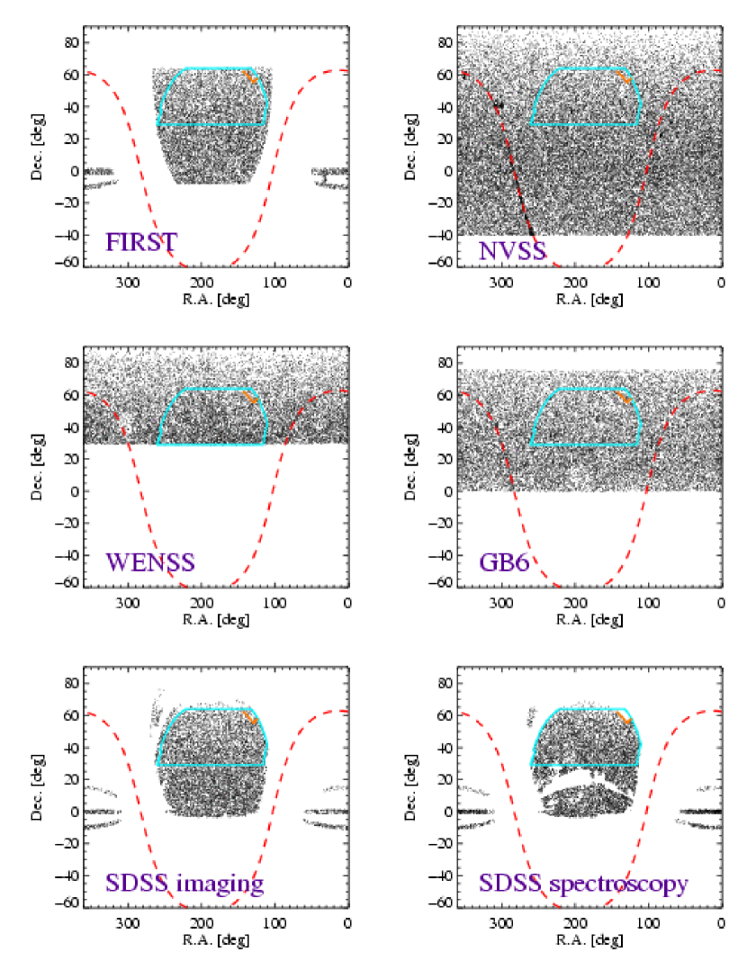
Figure 1: Using sparse sampling, we show the sky coverage of each of the surveys used to created the matched catalog. The blue line shows the $2955\deg^{2}$ region of overlap of the radio surveys and the SDSS photometric survey. The $2894\deg^{2}$ region outlined by the orange and blue lines shows the region included in the spectroscopic sample of SDSS DR6. The dashed red line indicates the Galactic plane.

The limits in sky coverage of the catalog are defined by the FIRST and NVSS sky coverage (Fig. 1). The unified catalog thus includes sources in the Galactic plane which are imaged by the NVSS. Galactic sources must be studied with care: due to the nature of interferometry, radio surveys (depending on their angular resolution) generally do a poor job of imaging highly-extended sources such as Galactic HII regions and supernova remnants, whose angular sizes often reach several arcmin or more. The analysis presented in this paper is limited to the sky covered by FIRST, which is greater than $30\arcdeg$ from the Galactic plane.

In this paper, we discuss scientific applications of the unified radio catalog and present a preliminary data analysis. In a companion paper (A. Kimball et al. in preparation), we will expand upon and refine this analysis by comparing the source distribution in radio morphology, radio color, and optical classification space to the models of Barai & Wiita (2006, 2007).

The remainder of the paper is laid out as follows. In §2, we describe the surveys used to create the unified radio catalog. In §3 we discuss the creation of the catalog, including completeness and efficiency of the matching algorithms. In §4 we present a preliminary analysis of the radio source distribution according to radio morphology, radio color, optical identification, and, for sources with spectra, redshift and luminosity. We also discuss some catalog applications. We summarize our results, and discuss the suitability of the catalog for comparison with radio evolution models, in §5.

2 SOURCE SURVEYS

Before proceeding with a description of merging procedure for the FIRST and NVSS catalogs, we briefly describe each survey used in creating the multi-wavelength radio catalog, including the sky coverage, wavelength, astrometric accuracy, and flux limit (see Table 1 for summary). Sky coverage of each survey is shown in Figure 1. The region of sky observed by all of the contributing surveys is indicated by the cyan solid line.

2.1 Radio surveys

2.1.1 FIRST

The FIRST survey (Faint Images of the Radio Sky at Twenty centimeters; Becker et al., 1995) used the VLA to observe the sky at 20 cm (1.4 GHz) with a beam size of 5$\farcs$4 and an rms sensitivity of about 0.15 mJy beam^-1. Designed to cover the same region of the sky as the SDSS, FIRST observed $9,000\deg^{2}$ at the north Galactic cap and a smaller $\sim 2.5\arcdeg$ wide strip along the Celestial Equator. It is 95% complete to 2 mJy and 80% complete to the survey limit of 1 mJy. The survey contains over 800,000 unique sources, with astrometric uncertainty of $\lesssim 1\arcsec$. FIRST includes two measures of 20 cm continuum flux density: the peak value, $F_{\mathrm{peak}}$, and the integrated flux density, $F_{\mathrm{int}}$, measured by fitting a two-dimensional Gaussian to co-added images of each source.

2.1.2 NVSS

The NVSS (NRAO-VLA Sky Survey; Condon et al., 1998) was also carried out using the VLA radio telescope to observe the sky at 20 cm (1.4 GHz), the same wavelength as FIRST. However, the NVSS used a different antenna configuration, resulting in a lower spatial resolution ($45\arcsec$ beam^-1). Lower resolution radio surveys provide more accurate flux measurements for extended sources, where high-resolution surveys can miss a significant fraction of the flux. The astrometric accuracy ranges from $1\arcsec$ for the brightest NVSS detections to about $7\arcsec$ for the faintest detections. The survey covers the entire sky north of $\delta=-40\arcdeg$ and contains over 1.8 million unique detections brighter than 2.5 mJy.

For the analysis of this paper, we adopt integrated NVSS flux densities rather than the peak flux densities reported in the NVSS catalog. Condon et al. (1998) provides formulas for converting peak flux densities to integrated flux densities, as well as formulas for errors in NVSS measured and calculated values. The unified catalog includes the integrated NVSS flux density, the corrected peak flux density, and the deconvolved major and minor axis sizes.

2.1.3 WENSS

WENSS (Westerbork Northern Sky Survey; Rengelink et al., 1997) is a 92 cm (325 MHz) survey completed with the Westerbork Synthesis Radio Telescope. It maps the radio sky north of $\delta=29\arcdeg$ to a limiting flux of 18 mJy, with a beam size of $54\arcsec\times 54\arcsec\mathrm{cosec}(\delta)$. The complete survey contains almost 220,000 sources, with a positional uncertainty of $\lesssim 1.5\arcsec$ for bright sources and $\lesssim 5\arcsec$ for faint sources.

2.1.4 GB6

The GB6 survey at 4.85 GHz (Green Bank 6 cm survey; Gregory et al., 1996) was executed with the (now defunct) 91m Green Bank telescope in 1986 November and 1987 October. Data from both epochs were assembled into a survey covering the $0\arcdeg<\delta<75\arcdeg$ sky down to a limiting flux of 18 mJy, with $3.5\arcmin$ resolution. GB6 contains over 75,000 sources, and has a positional uncertainty of about $10\arcsec$ at the bright end and about $50\arcsec$ for faint sources.

2.2 Optical Surveys: SDSS

We use photometric and spectroscopic coverage from the sixth data release (DR6) of the Sloan Digital Sky Survey (SDSS; see York et al., 2000; Stoughton et al., 2002; Adelman-McCarthy et al., 2007, and references therein). The survey, not yet finished but nearing completion, will eventually cover $10,000\deg^{2}$ in the northern galactic cap and a smaller region on the celestial equator. DR6 covers roughly $9,600\deg^{2}$, and contains photometric observations for 287 million unique objects, as well as spectra for more than 1 million sources.

2.2.1 The SDSS Photometric Survey

The SDSS photometric survey contains flux densities of detected objects measured nearly simultaneously in five wavelength bands ($u$, $g$, $r$, $i$, and $z$; Fukugita et al., 1996) with effective wavelengths of 3551, 4686, 6165, 7481, and 8931Å (Gunn et al., 1998). The catalog is 95% complete for point sources to limiting AB magnitudes of 22.0, 22.2, 22.2, 21.3, and 20.5 respectively. Typical seeing is about $1.4\arcsec$ and positional uncertainty is less than about $0.1\arcsec$ (rms per coordinate for sources with $r<20.5$, Pier et al., 2003). The photometry is repeatable to 0.02 mag (rms for sources not limited by photon statistics, Ivezić et al., 2003) and with a zeropoint uncertainty of $\sim$0.02-0.03 mag (Ivezić et al., 2004a). A compendium of other technical details about SDSS can be found on the SDSS web site, which also provides an interface for public data access.

Optical magnitudes in this paper refer to SDSS model magnitudes, measured using a weighting function determined from the object’s $r$ band image (see Stoughton et al., 2002). The weighting function represents the better fitting of an exponential profile and a de Vaucouleurs profile. The chosen model is then used to determine the magnitude in all five bands. We corrected all magnitudes for Galactic extinction following Schlegel et al. (1998). When selecting candidate matches from the SDSS, we required unique sources that are brighter than $r=22.2$ or brighter than $z=21.2$.

The morphological information from SDSS images allows reliable star-galaxy separation to $r\sim 21.5$ (Lupton et al., 2002; Scranton et al., 2002). In brief, sources are classified as resolved or unresolved according to a measure of light concentration that represents how well the flux distribution matches that of a point source (Stoughton et al., 2002). As sources that emit strongly in the radio are almost exclusively extra-galactic at the high latitudes observed by the SDSS ($|b|>30$), this classification effectively divides radio sources into “galaxies” (resolved) and “quasars” (unresolved). The optically-unresolved sources may also include a small number of galaxies that are unresolved in the SDSS images, as well as a small fraction of radio stars. For the remainder of this paper, we refer to the two sets of photometric optical sources (as opposed to those with available spectra, see below) as “galaxies” and “optical point sources”.

2.2.2 The SDSS Spectroscopic Survey

A subset of photometric sources are chosen for spectroscopic observation according to the SDSS’s spectral target selection algorithms. Targeted extragalactic sources include the flux-limited “main” galaxy sample ($r<17.77$; Strauss et al., 2002), the luminous red galaxy sample (Eisenstein et al., 2001), and quasars (Richards et al., 2002). DR6 contains spectra for about 100,000 quasars and 790,000 galaxies. The spectral wavelength range is $3800-9200$Å, with a resolution of 1800 and redshift accuracy of 30 km s^-1 (estimated from the main galaxy sample).

The main galaxy sample includes nearly all ($\sim 99\%$) galaxies brighter than $r<17.77$, resulting in a sky density of $\approx 90\deg^{-2}$. Some targets are rejected on the basis of low surface brightness (where redshifts become unreliable or targets are spurious) or high flux (which can contaminate neighboring fibers). Due to the physical thickness of the spectral fibers, two galaxies closer than $55\arcsec$ cannot be observed at the same time, although overlapping spectral plates allow some initially-skipped galaxies to be picked up later. A second galaxy target algorithm selects luminous red galaxies (LRGs; Eisenstein et al., 2001), which are typically the brightest members of galaxy clusters. LRG targets are selected primarily by color, based on known LRG spectra at different redshifts. The resulting sample is typically more luminous and much redder than the main galaxy sample, and extends to fainter apparent magnitudes than the main sample.

The quasar target selection algorithm (Richards et al., 2002) selects targets from unresolved objects with $i<19.1$ and colors similar to redshift $\lesssim 3$ quasars, unresolved objects with $i<20.2$ and colors similar to higher redshift quasars, and unresolved sources within $2\arcsec$ of a FIRST source ($i<19.1$). The completeness of the sample is $\approx 95\%$ and the selection efficiency is $\approx 66\%$. Contamination is much higher than for the galaxy sample: the latter consists of resolved sources, which are thus nearly always galaxies, whereas the quasar sample is contaminated by non-quasar point sources, such as distant galaxies or Galactic stars with quasar-like colors. In fact, nearly 30% of the targets turn out to be stars.

To distinguish the spectroscopic SDSS sample from the photometric SDSS sample, we refer to sources from the former as “spectroscopic galaxies” and “spectroscopic quasars”.

3 THE UNIFIED CATALOG

The cross-identification of radio surveys at different wavelengths, and with different resolutions, is not a straightforward task (Becker et al., 1995; Ivezić et al., 2002; de Vries et al., 2006; Lu et al., 2007). However, the accurate astrometry of FIRST allows simple positional matching to the other radio surveys, and to the optical SDSS, with high completeness and low contamination. Catalog entries are defined by a detection in at least one of the two 20 cm surveys (FIRST and NVSS). Where available, the 20 cm data is supplemented with 92 cm and 6 cm radio data, from WENSS and GB6, and with optical observations from the SDSS.

In the remainder of this section, we describe the matching technique used to create the unified radio catalog. The complicated procedure outlined herein is intended to include all objects with even a small chance of being physically-real associations. Therefore, catalog users are not limited to the matching techniques or matching distances used by the authors in the subsequent analysis in this paper. The generous matching radii used to create the catalog can easily be restricted by future users using the catalog parameters detailed in Appendix A.

3.1 Defining catalog entries from the FIRST and NVSS surveys

FIRST and NVSS both observed the sky at 20 cm (1400 MHz). Of the four radio surveys incorporated into the unified catalog, these two have the faintest flux limits and the highest spatial resolution, with FIRST having even higher resolution than NVSS. Radio surveys necessarily involve a trade-off between high resolution, which allows for accurate determination of positions, and low resolution, which allows for the detection of low surface brightness sources and complete flux measurements for extended sources. By combining high-resolution FIRST with the lower-resolution NVSS, it is possible to achieve the best of both options. FIRST provides accurate positional measurements, and the NVSS provides accurate flux measurements for extended and low-surface brightness sources, where FIRST underestimates the radio flux (Becker et al., 1995; Lu et al., 2007).

3.2 Matching algorithm for the radio surveys

Due to different spatial resolution and faint limits, combined with the complex morphology of radio sources, the positional matching of FIRST and NVSS sources cannot be done in an a priori correct way. For this reason, we adopt a flexible method that enables later sample refinement after the initial positional association. The unified catalog contains the three closest FIRST matches to an NVSS source within $30\arcsec$, and the three closest NVSS matches to a FIRST source within $30\arcsec$. For each source, we also record the total number of matches found within $5\arcsec$, $10\arcsec$, $30\arcsec$, and $120\arcsec$, which will allow users to investigate radio properties as a function of environment density. The complete catalog contains over 2.7 million entries, including FIRST-NVSS associations, isolated FIRST or NVSS sources, and NVSS sources that lie outside the FIRST survey coverage. Because we match FIRST to NVSS and then NVSS to FIRST, there are necessarily duplicate catalog entries: for example, a very close match will appear once as a FIRST to NVSS match and once as a NVSS to FIRST match. However, the catalog includes parameters to easily extract specific data samples, including the elimination of any duplicates. Similarly, the processing flags can be used to treat cases such as distinct FIRST sources matched to the same NVSS source (and vice-versa, although the latter case is rare due to the lower spatial resolution and brighter limit of NVSS). For further details, we refer the reader to Appendix A.

Measured FIRST and NVSS sky positions are rarely exact even for the same source. As shown in Figure 2, FIRST has more accurate astrometric measurements than NVSS, due to its higher spatial resolution. We therefore use FIRST to designate the sky position of each catalog entry, when possible. For NVSS sources without a FIRST match, we retain the NVSS coordinates. The designated position is then used when searching for counterparts in the other surveys.

To match the FIRST and NVSS surveys, we use a matching radius of 30″. We use a larger radius of $120\arcsec$ to match to WENSS and GB6, since they both have lower positional accuracies. We also record the total number of WENSS and GB6 matches found within $120\arcsec$. All of the matching radii used to create the catalog are generously large, to ensure that the majority of physically-real matches are included. To select smaller, cleaner samples for analysis, the catalog user can choose matches based on distance, effectively applying a smaller matching radius. The contamination and completeness as a function of matching radius are discussed in §3.4.

The surveys used in the creation of the unified catalog are themselves catalogs of individual radio components. Thus, large multi-component physical sources can be resolved into separate detections in the high angular-resolution surveys, particularly in FIRST ($5\arcsec$ resolution), but also in NVSS and WENSS ($\sim 50\arcsec$ resolution). Best et al. (2005, hereafter B05) developed a clean sample of double-lobed radio-loud galaxies by matching radio components to spectroscopic SDSS galaxies. B05 used the optical core position and the optical galaxy alignment to eliminate unlikely lobe-configurations, based on lobe opening angles and distances. The complexity of a matching algorithm based only on radio components, as presented in this paper, is necessarily much greater because the optical position of the core is unknown for the majority of sources. We therefore settle on the matching scheme outlined above, which allows sample selection with the user’s own preferred matching criteria, without the need to repeat the work that has gone into developing the unified catalog presented here.

3.3 Matching algorithm for the SDSS

We correlate the matched radio sources with the SDSS photometric survey, including spectroscopic data when available, using a matching radius of $60\arcsec$. In addition to the nearest neighbor, the catalog includes the brightest neighbor within a pre-defined radius ($3\arcsec$, $10\arcsec$, $30\arcsec$, or $60\arcsec$; see Appendix A for details). The total number of matches within the same pre-defined radius is also recorded, indicating optical source sky density at each entry’s location.

We note that some lobe-dominated radio sources may be missed when positionally matching SDSS and FIRST source positions. While each radio lobe will be included individually in the radio sample, it will be excluded from the optically-matched subset for lobe-core distances larger than the SDSS matching radius. Lu et al. (2007) estimated that about 8.1% of radio quasars do not show a radio core within $2\arcsec$ of their optical position, and thus would be missed by this algorithm. However, Ivezić et al. (2002) and de Vries et al. (2006) found fewer than 5% and 2%, respectively, of quasars are double-lobed in FIRST, using optical core positions without assuming radio emission in the core. Because NVSS has a much larger spatial resolution than FIRST, even fewer double-lobed sources can be expected in NVSS. B05 found 6% of their spectroscopic SDSS galaxies to be double-lobed in NVSS. Note that while the percentage is larger for galaxies, as expected from orientation effects, this value is an upper limit for radio-optical samples using photometric optical data, as the spectroscopic SDSS sample is comprised of the nearest sources, which thus have large angular size. Since the effect is not overwhelming, the unified catalog only includes direct positional matches between SDSS and radio (FIRST or NVSS) catalogs. However, catalog users can easily repeat the procedures for finding double-lobed sources developed by Ivezić et al. (2002); de Vries et al. (2006); Best et al. (2005), which would involve matching external optical samples to the radio catalog sources.

3.4 Completeness and efficiency of matched samples

A side effect of using large matching radii is increased contamination by coincidental “line-of-sight” matches to physically unrelated objects. Using the nearest-neighbor distributions, we estimate efficiency (fraction of matches which are physically real) and completeness (fraction of real matches that were found) as a function of matching radius. Figure 3 shows the distribution of distances between FIRST sources and the nearest neighbor from the NVSS, WENSS, GB6, and SDSS (photometric) surveys. For comparison, it also shows the estimated level of background contamination. The nearest-neighbor distributions peak at small distances, where associations are likely to be real, then decrease sharply; the width of the peaks depends on the astrometric accuracy of the corresponding surveys. The distributions slowly rise again at large distances due to increased background contamination. Efficiency and completeness are estimated using a model fit to the nearest neighbor distributions. Estimated values of completeness and efficiency based on the model fitting are listed in Table 2. For the samples discussed here, typical values are $>90\%$ completeness and $>80\%$ efficiency.

As discussed above, the unified catalog includes individual radio components, and does not correctly handle NVSS multi-component sources. Two lobes from a very large ($\gtrsim 100\arcsec$) source may appear as two detections in NVSS and thus in the unified catalog as well. The values in Table 2 show that when matching up individual radio components between different surveys, the completeness is well over 90%. As stated in §3.3, investigations using optical and radio surveys suggest that only a few per cent of radio sources are double-lobed in FIRST; much smaller percentages are expected in the NVSS. Indeed, B05 note that the NVSS resolution is large enough that $\sim 99\%$ of radio sources are contained in a single NVSS component. Although the missing double-lobed sources are not addressed further in this paper, we tackle the issue in the companion paper, where we thoroughly discuss the classification of a WENSS-NVSS-FIRST subsample (see §5.4.1 for discussion). It will include the missing double-lobed sources, found by determining the complete NVSS-FIRST environment around each WENSS object, requiring extensive visual analysis.

3.5 FIRST matching statistics

Of the four radio surveys used to create the unified catalog, FIRST extends to the faintest flux limit. We discuss here the likelihood of finding a FIRST source in one or more of the other three radio surveys. In this section and for the remainder of this paper, we limit our analysis to the common region observed by all of the contributing surveys (see Fig. 1).

The number of matches found between different surveys is a strong function of source flux. The flux range of objects in the unified catalog covers several orders of magnitude. Thus, for convenience we convert radio flux to an “AB radio magnitude”, following Ivezić et al. (2002):

$$t_{\mathrm{radio}}=-2.5\log\left(\frac{f_{\mathrm{int}}}{3631\,\mathrm{Jy}}\right),$$ (1)

where $f_{\mathrm{int}}$ is the integrated flux density. This formula places the radio magnitudes on the $\mathrm{AB}_{\nu}$ system of Oke & Gunn (1983). An advantage of that system is that the zero point (3631 Jy) does not depend on wavelength and thus enables convenient data comparison over a large wavelength range. For example, a source with a radio flux of 1 mJy has $t_{\mathrm{radio}}=16.4$; if it has constant $F_{\nu}$ (a flat spectrum), its visual magnitude is also $V=16.4$.

Figure 4 shows the magnitude distribution for FIRST sources with and without radio matches from the other surveys. Each panel roughly indicates the $t_{\mathrm{FIRST}}$ magnitude corresponding to the other survey’s faint limit. For example, the fraction of FIRST sources with a counterpart in NVSS is greater than 0.9 at $t_{\mathrm{FIRST}}=15$ but drops to 0.5 at $t_{\mathrm{FIRST}}=15.5$ as shown in Panel A, indicating that the NVSS faint limit corresponds to $t_{\mathrm{FIRST}}\approx 15$. The sensitivity limit of GB6, $t_{\mathrm{GB6}}=13.3$, occurs at $t_{\mathrm{FIRST}}\approx 12$ (panel B). The limit is brighter in FIRST than GB6 because, as is well known and as we confirm with a much larger sample in §4.2, most radio sources are intrinsically fainter at 6 cm than at 20 cm (in terms of $F_{\nu}$; i.e. corresponding faint limits depend on spectral slope). Requiring a GB6 detection therefore biases a sample to the brightest sources. Panel C shows that the WENSS faint limit, $t_{\mathrm{WENSS}}=13.3$, corresponds to a limit of $t_{\mathrm{FIRST}}\approx 14$, because radio sources are, again on average, intrinsically brighter at 92 cm than at 20 cm.

Roughly 60% of FIRST sources have an NVSS counterpart within $30\arcsec$. Of those radio sources observed by both surveys ($\approx 48\deg^{-2}$), 50% have a WENSS counterpart and 12% have a GB6 counterpart within $120\arcsec$, while 11% have both. The sky density of sources observed by all four radio surveys is $\approx 5.3\deg^{-2}$, or $\sim 5\%$ of the FIRST source density.

3.5.1 NVSS sources without a FIRST counterpart

Because FIRST goes fainter than the NVSS by a factor of 2.5, there are many FIRST sources without an NVSS counterpart ($\sim 38\deg^{-2}$, see Panel A of Fig. 4; $\sim 0.53\deg^{-2}$ for FIRST sources brighter than 10 mJy). However, the catalog also contains some NVSS sources without a FIRST counterpart ($\sim 7.8\deg^{-2}$; $\sim 0.56\deg^{-2}$ for sources brighter than 10 mJy). For an astronomical object to be detectable by NVSS but not FIRST, it must be large and have a surface brightness too faint for the high-resolution FIRST survey. On the other hand, it is possible that NVSS sources without FIRST counterparts are simply spurious, or have badly measured NVSS positions, i.e. their FIRST counterparts are outside the $30\arcsec$ matching radius. The top panel of Figure 5 shows the nearest neighbor distribution from the WENSS catalog for NVSS sources lacking a FIRST counterpart within $30\arcsec$. It peaks at small distances due to physically-associated objects, demonstrating that NVSS sources lacking a FIRST counterpart but with a WENSS match (within $55\arcsec$), are dominated by real sources. If these are not spurious detections, they belong to the category of extended, low-surface brightness objects missed by the high-resolution FIRST.

Assuming that real NVSS sources have a counterpart in at least one of FIRST and WENSS, we estimate an upper limit for the fraction of spurious NVSS detections. Nearly 14% of NVSS objects in the region of survey overlap have no FIRST counterpart within $30\arcsec$, and 12.2% have no FIRST or WENSS counterpart, the latter within $55\arcsec$. NVSS has a much fainter flux limit than WENSS (2.5 mJy as opposed to 18 mJy): sources near the NVSS faint limit are likely to fall below the WENSS faint limit. For the sample of NVSS detections brighter than 18 mJy, only 0.43% lack both FIRST and WENSS counterparts, which we interpret as an upper limit on the fraction of spurious NVSS sources. The selection on which we base this estimate is biased against sources brighter at 20 cm than at 92 cm; however, this type of radio source is rare, as we later show (§4.2). According to de Vries et al. (2002), NVSS begins to lose completeness below 12 mJy. We find that 2.3% of NVSS sources above this limit have no FIRST match.

3.6 Catalog availability

The full catalog and several pre-made subsets are available for download on the catalog website, which also provides a list and description of the data parameters. The datasets are described in Appendix B. All 2,724,343 rows of the complete catalog (sample A) are available in a tarred archive of fits files, each covering a $5\arcdeg$ wide strip in right ascension. A small subset of the catalog selected from $\approx 100\deg^{2}$ of sky, with 16,453 rows (sample B), allows users to familiarize themselves with the data format. Several scientifically-useful subsets of the catalog are pre-made for convenience; some of these are analyzed in the next section. The first of these subsets contains radio fluxes and positions for NVSS-FIRST associations (sample C), including 6 and 92 cm data, while another contains sources matched by all four radio surveys as well as the SDSS (sample F). Two more subsets consist of spectroscopic galaxies (sample G) and spectroscopic quasars (sample H), detected by NVSS, FIRST, WENSS, and SDSS. Also provided are a sample of isolated FIRST-NVSS sources (sample I) and isolated FIRST-NVSS-SDSS sources (sample J). Finally, a set of high-redshift galaxy candidates is available (sample K; see §5.2). A more detailed description of these data files can be found in Appendix B.

4 PRELIMINARY CATALOG ANALYSIS

In this section, we investigate the distribution of sources in radio color-magnitude-morphology parameter space. We define the relevant morphology and spectral parameters using five radio fluxes: peak FIRST flux (20 cm), integrated FIRST and NVSS fluxes (20 cm), GB6 flux (6 cm), and WENSS flux (92 cm). While the unified catalog contains many more useful parameters inherited from the original catalogs, in this preliminary analysis we focus only on these few. We use FIRST and NVSS flux measurements to define two morphology estimators, and use GB6 and WENSS fluxes with NVSS flux to compute radio spectral slopes. Morphology estimators are used to define three morphology classes, for which we construct radio “color-magnitude” diagrams. We also utilize optical photometric identification in the analysis, classifying sources as SDSS point sources, extended sources, or faint sources (non-detections).

Hereafter our discussion covers samples selected using the conservative matching radii listed in Table 2. We settle upon these values by looking for an optimal balance between completeness and efficiency of the matched samples, as illustrated in Fig. 3. The matching radii used herein are as follows, with the larger values for all catalog associations given in parentheses: FIRST-NVSS, $25\arcsec$ ($30\arcsec$); FIRST-WENSS, $30\arcsec$ ($120\arcsec$); FIRST-GB6, $70\arcsec$ ($120\arcsec$); FIRST-SDSS, $2\arcsec$ ($60\arcsec$). Estimated values of completeness and efficiency, calculated by comparing with random matching, are listed in Table 2.

Our analysis is limited to the $2955\deg^{2}$ region where the contributing surveys overlap (Fig. 1) in order to control the selection criteria of the analyzed samples. There are nearly 490,000 catalog entries in the overlap region, including multiple FIRST components matched to the same NVSS source, as well as duplicate entries (see §3.2). To obtain a sample of physical FIRST-NVSS associations, it is sufficient to select catalog entries containing an NVSS source and its nearest FIRST match: individual objects are typically not resolved into multiple components in NVSS because of the survey’s larger beam. This method selects $\sim 140,000$ unique, likely physical NVSS-FIRST associations. Of those, $\sim 64,000$ are matched to a WENSS source, $\sim 14,000$ to a GB6 source and $\sim 48,000$ to an SDSS source.

4.1 Morphology classification of radio sources

4.1.1 “Simple” vs. “complex” FIRST-NVSS sources

FIRST is a high-resolution interferometric survey, and thus underestimates the flux of extended and lobe-dominated sources (Becker et al., 1995; Lu et al., 2007). Additionally, a multiple-component source with core and lobes may be detected as three objects by FIRST but as only a single object in the lower-resolution NVSS. The difference between the two 20 cm magnitudes is thus a measurement of source morphology that indicates angular extent and complexity. We define

$$\Delta t=t_{\mathrm{FIRST}}-t_{\mathrm{NVSS}}.$$ (2)

Before applying $\Delta t$ as a classifier we investigate its dependence on $t_{\mathrm{NVSS}}$ for NVSS-FIRST pairs (sample C) in Figure 6. The distribution in $\Delta t$ is bimodal, with the two peaks centered at $\Delta t=0$ and $\Delta t=0.7$. Through the visual inspection of a thousand FIRST images (see below, §4.1.3), we verified that sources in the $\Delta t\sim$ locus are single component sources, while those in the $\Delta t\sim.7$ locus are multiple-component or extended. The lower panel shows the $\Delta t$ distribution for four magnitude bins. We fit the sum of two Gaussians to each of the four distributions; best-fit parameters are listed in Table 3. The $\Delta t$ distribution is similar for all magnitudes, although the overlap between the two peaks increases for fainter sources as flux measurement errors increase. We adopt $\Delta t=0.35$ (solid horizontal line) as the separator between “simple” ($\Delta t<0.35$) and “complex” ($\Delta t>0.35$) sources.

4.1.2 “Unresolved” vs. “resolved ” FIRST sources

The ratio of the two FIRST flux measurements—peak and integrated—yields a second measure of morphology: a dimensionless source concentration on $\sim 5\arcsec$ scale. We define

$$\theta=\left(\frac{F_{\mathrm{int}}}{F_{\mathrm{peak}}}\right)^{1/2}.$$ (3)

Sources with $\theta\sim$ are highly concentrated (unresolved), while sources with larger $\theta$ are extended (resolved). We adopt $\log(\theta^{2})=0.05$ ($\theta\approx 1.06$) as the value separating resolved and unresolved sources. This choice is motivated by the distribution of sources in the two-dimensional $\Delta t$ vs. $\theta$ distribution, discussed below.

4.1.3 Automatic morphology classification of radio sources

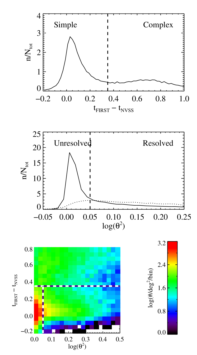
Figure 7: Top: Distribution of $\Delta t$ for sources with $t_{\mathrm{NVSS}}<13.5$. The dashed line indicates the separation between the simple and complex morphology classes. Middle: Distribution of $\theta$, an estimate of source size. The solid curve corresponds to simple sources; the dotted curve corresponds to complex sources. The vertical line separates unresolved and resolved sources at 20 cm. Bottom: Distribution of $\Delta t$ vs. $\log\theta^{2}$ for sources with $t_{\mathrm{NVSS}}<13.5$. The dashed lines indicate the adopted separation of morphology classes: the complex sample is above the horizontal dashed line, the compact sample is left of the vertical dashed line, and the resolved sample is to the right of the vertical dashed line.

The two-dimensional $\Delta t$ vs. $\theta$ distribution for sources with $t_{\mathrm{NVSS}}<13.5$ (the brightest 30% of NVSS-FIRST pairs) is illustrated in Figure 7, along with the marginal distributions for the two morphology parameters. The distribution in the lower panel suggests that 20 cm radio fluxes can be used to automatically separate FIRST-NVSS detections into three morphology classes: “complex”, (simple) “resolved”, and (simple) unresolved or “compact”.

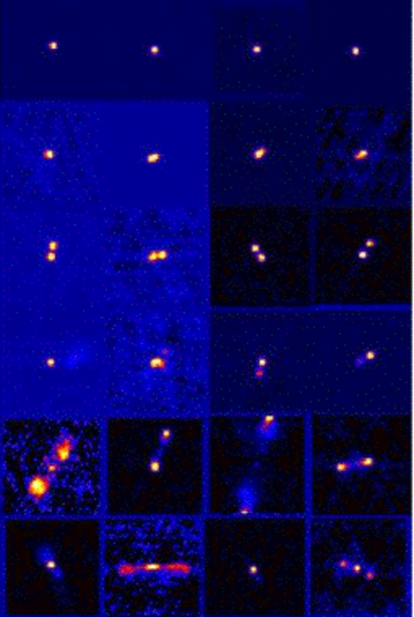
Figure 8: Examples of radio sources classified by morphology (FIRST $1\arcmin\times 1\arcmin$ stamps normalized to the brightest pixel, shown with square root stretch). The top row contains compact radio sources, the second row shows resolved sources, and the remainder are complex. The left two columns show sources optically identified as galaxies by the SDSS; the right two columns show SDSS-identified quasars.

This assertion was verified by extensive visual inspection of FIRST images (Fig. 8). Over 1000 FIRST stamps ($2\times 2~{}\mathrm{arcmin}^{2}$) of optically-identified radio quasars and radio galaxies were classified both visually and automatically (as above) into “complex”, “resolved”, and “compact” categories. A comparison of the results is given in Table 4. The two methods are consistent: over three quarters of all sources (81% of quasars and 76% of galaxies) receive identical classification from the two methods. Two initially surprising results are the significant fraction of objects classified as “complex” by one method and “compact” by the other. In particular, 15% of visually-complex quasars were automatically classified as “compact”. As it turns out, the majority of these sources appear (by eye) to be asymmetric double-lobed sources with a very high flux ratio. Their FIRST images show two lobes, hence the visual “complex” classification. However, their total flux is due primarily to the brighter lobe, meaning FIRST and NVSS flux measurements are similar, resulting in an automatic classification of “compact”. Additionally, 26% of visually-compact galaxies were classified automatically as “complex”. An inspection of flux values reveals that many of these are borderline cases, with $\Delta t$ value just above the $\Delta t=0.35$ cutoff. It is likely that these galaxies have faint, diffuse emission which is detected by the NVSS but is not visible in the FIRST images.

The automatic morphology classification presents difficulties because of non-unique pair matching, e.g. multiple FIRST detections matched to a single NVSS object. The resolved/unresolved classification is based on FIRST fluxes and therefore applies to FIRST components individually. In choosing an analysis sample based on FIRST-NVSS pair matching, we retain only the closest FIRST match to an NVSS object (see Appendix A for details). The fluxes of the closest FIRST match are used, while more distant FIRST sources are ignored, when classifying a FIRST-NVSS pair as resolved/unresolved. Approximately 17% of NVSS detections in the FIRST footprint have multiple FIRST matches within 30″. Most of these sources (88%) are classified as complex, presumably because the NVSS flux encompasses multiple FIRST components. We therefore apply the resolved/unresolved classification only to “simple” sources, resulting in the three morphology classifications. (In other words, we do not separate the complex sources into “complex resolved” and “complex unresolved”.)

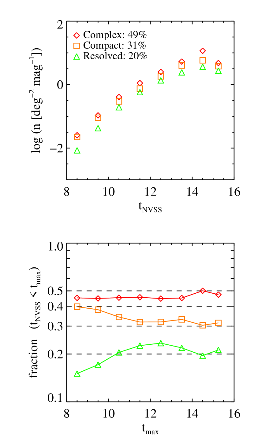
Figure 9: Top: Distribution of NVSS-FIRST sources classified according to radio morphology, as a function of $t_{\mathrm{NVSS}}$. Bottom: Fraction of sources brighter than $t_{\mathrm{max}}$ belonging to each morphology class.

Figure 9 shows the magnitude distribution for NVSS-FIRST associations of each morphology class, and the fraction in each class of all sources brighter than a limiting $t_{\mathrm{NVSS}}$ magnitude. There are similar numbers of complex and compact sources at all magnitudes; there are fewer resolved sources, and the fraction increases slightly at fainter flux values. Overall, the fractions remain roughly constant with flux. In the next section, we investigate correlations between radio morphology and radio spectral slope.

4.2 Radio color-magnitude and color-color diagrams

In the previous section, we described an automatic morphology classification for NVSS-FIRST associations based on their 20 cm fluxes. The addition of WENSS (92 cm) and GB6 (6 cm) data allows us to compute radio spectral slope, and to study its correlation with radio morphology and magnitude.

For two magnitudes $t_{1}$ and $t_{2}$, we compute a spectral index $\alpha$, defined by $F_{\nu}\propto\nu^{\alpha}$, as

$$\alpha^{t_{1}}_{t_{2}}=\frac{0.4}{\log(\lambda_{t_{1}}/\lambda_{t_{2}})}(t_{1}-t_{2}).$$ (4)

The value $\alpha$ describes the average spectral slope between wavelengths $\lambda_{t_{1}}$ and $\lambda_{t_{2}}$; it is proportional to the color $t_{1}-t_{2}$. Therefore

$$\alpha^{20}_{6}=0.765(t_{\mathrm{NVSS}}-t_{\mathrm{GB6}}),$$ (5)

$$\alpha^{92}_{6}=0.337(t_{\mathrm{WENSS}}-t_{\mathrm{GB6}}),$$ (6)

and

$$\alpha^{92}_{20}=0.604(t_{\mathrm{WENSS}}-t_{\mathrm{NVSS}}).$$ (7)

Note that we use NVSS rather than FIRST when calculating spectral indices for the analysis presented here, as NVSS is more likely to detect all the 20 cm flux from a source due to its larger beamsize.

Typical extragalactic radio sources have spectral index in the range $-1<\alpha<0$ in the radio regime (e.g., Condon, 1984; Blundell et al., 1999), with $\alpha=-0.5$ as a typical value separating steep-spectrum and flat-spectrum sources (e.g., Urry & Padovani, 1995). Emission from extended radio lobes, such as those seen in classical FR2 objects (Fanaroff & Riley, 1974) tends to be steeper, with the steepening attributed to synchrotron, inverse Compton, and adiabatic losses acting on the relativistic electrons. The flatter emission from compact quasar cores/jets is interpreted as self-absorbed synchrotron emission (Krolik, 1999). As described in Jarvis & McLure (2006), radio spectral index is thought to correlate with source orientation in AGN unification schemes: sources viewed along the jet axis show flat radio spectra, sources viewed along the dust torus show steep radio spectra (since only the lobes are visible), and intermediate orientations result in intermediate spectral slopes due to mixing of the flat- and steep-spectrum emission. A minority of observed radio sources fall into the gigahertz-peaked-spectrum (GPS; 10%) and compact-steep-spectrum (CSS; 30%) categories (O’Dea, 1998). GPS and CSS sources are similar to smaller versions of FR2s, but have convex spectra that peak around 1 GHz in the observer frame.

Two significant systematic issues could cause errors in our measure of radio spectral index. The first of these is the possible variability in radio flux over the timescale of the survey observations: GB6 observations were carried out in 1986 and 1987, WENSS operated in the early 1990s, and NVSS observations were taken in the first half of 1998. AGN have shown flux variations over all radio wavelengths on timescales ranging from less than a day to years. Intrinsic variability is thought to be due to jet variations, such as shocks propagating along the jet (Marscher & Gear, 1985; Hughes et al., 1989), with Doppler boosting acting to exaggerate the effect. Therefore, variability should be more prevalent in sources viewed along or near the jet axis, which is consistent with observations: blazars, quasars, flat-spectrum sources, and compact sources show higher variability among a greater fraction of sources than control samples. For example, Barvainis et al. (2005) observed variability at the 5-8% level over a two-year timescale for core-dominated quasars observed at 8.4 GHz. They also observed some large variations on month-long timescales, but only one in five of their sources varied at the 10-30% level, and most varied by less than 20%. Meanwhile, de Vries et al. (2004) found that roughly 2% of their sample of unresolved FIRST sources show significant variability ($>4\sigma$). In a sample of 3600 sources brighter than 0.1 mJy at 1.4 GHz, Rys & Machalski (1990) found that less than 1% were variable, and that all of those have flat radio spectra, with 86% being core-dominated sources. As far as measurements for individual sources are concerned, a 10% flux variation at one of the two relevant wavelengths corresponds to a change of 0.08 in spectral index, while a 30% flux variation corresponds to a change of about 0.2 in spectral index. Results from the literature discussed above suggest that about 1% of the unified catalog sources varied significantly over the range of survey observations, and that the variation tended to be at the 10% level. Those sources are likely to be concentrated in the compact radio morphology sample with flat radio spectra ($\alpha\gtrsim-0.5$). This variability contributes to scatter in the distribution of $\alpha$.

The second issue which may cause erroneous calculations of spectral index is the fact that the radio surveys have different spatial resolutions. WENSS and NVSS both have $\sim 50\arcsec$ resolution (see Table 1), while GB6 has a resolution of about $200\arcsec$, and therefore gathers flux from a much larger area. This issue will effect $\alpha^{20}_{6}$ spectral index for radio sources resolved into separate NVSS components, such as a double-lobed radio galaxy with lobe separation $\sim 100\arcsec$. If a single NVSS component contains only half of a source’s total 20 cm flux while GB6 sees all of the 6 cm flux, then $\alpha^{20}_{6}$ will be too shallow by almost 0.6 for that source. We note that since WENSS and NVSS have similar angular resolution, this issue is unlikely to significantly affect the $\alpha^{92}_{20}$ measurements.

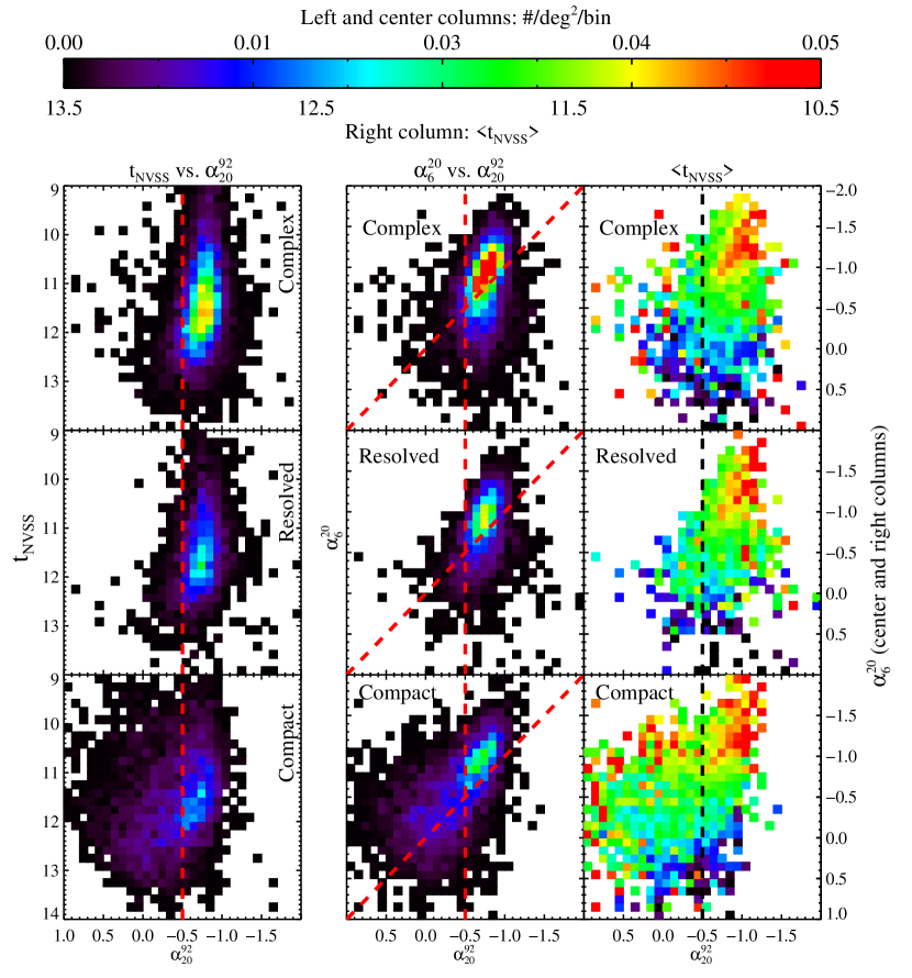
Figure 10: Color-magnitude (left), color-color (middle), and median magnitude (right) diagrams for sources detected in all four radio surveys and classified by radio morphology (top: complex; middle: resolved; bottom: compact). Vertical dashed lines show the $\alpha^{92}_{20}=-0.5$ separation between steep- and flat-spectrum sources in the 20-92 cm range. Left column: The distribution of NVSS magnitude vs. spectral slope $\alpha^{92}_{20}$. Center column: $\alpha^{20}_{6}$ vs. $\alpha^{92}_{20}$ color-color diagrams. The diagonal, dashed red lines show the $\alpha^{92}_{20}=\alpha^{20}_{6}$ locus. Right column: Color-color diagrams with bins color-coded according to the median value of NVSS magnitude $t_{\mathrm{NVSS}}$. The strong gradients in the right column are due to steep-spectrum sources, which are biased to bright sources by the shallow GB6 survey.

Figure 10 presents color-magnitude and color-color diagrams for the three radio morphology classes detected in all four radio surveys (listed as sample E in Appendix B). Similar color-color diagrams to those in the middle column were first presented in Ivezić et al. (2004a, Fig. 2), with slightly different selection criteria. The middle column demonstrates that the majority of sources in all three morphology classes have spectral indices $\alpha^{92}_{20}\approx\alpha^{20}_{6}\approx-0.8$. This result is in agreement with earlier observations (e.g., Kellermann, 1964; Laing et al., 1983; Zhang et al., 2003), and suggests that most strong radio sources have a fairly constant power-law slope from 6 to 92 cm. However, the radio compact sample (lower middle panel) has a significant fraction of flat-spectrum sources ($\alpha\sim 0$) as well. In the next section, we investigate the two groups of compact sources using optical identifications, and show that they are due to a population of galaxies and a population of optical point sources, with different distributions in radio color-color space. Note that in the color-color diagrams, the WENSS faint limit biases against large positive $\alpha$, while the GB6 limit biases against large negative $\alpha$. The strong correlation between $\alpha^{20}_{6}$ and $\left<t_{\mathrm{NVSS}}\right>$ in the right column is due to the GB6 survey sensitivity: only very bright steep sources are detected by GB6. A small fraction of sources ($<2\%$ with $t_{\mathrm{NVSS}}=12$) have a negative value for $\alpha^{92}_{20}$ but a positive value for $\alpha^{20}_{6}$, i.e. are fainter at 20 cm than at 92 cm and 6 cm. Such sources either have highly unusual radio spectra, or varied significantly in brightness over the range of observations.

We quantify the fraction of compact sources with steep and flat spectra in Figure 11. The sources are divided into four subclasses depending on their spectral shape between 6 cm and 92 cm. The top panel shows an example shape for each subclass. The “steep” and “flat” designations refer to sources with monotonic radio flux measurements. The middle panel shows the magnitude distribution of each subclass for compact sources with $t_{\mathrm{NVSS}}\leq 12$. Slightly less than two thirds of the compact sources are steep-spectrum, whereas 94% of complex and resolved sources are steep-spectrum. We find that one quarter of compact sources are flat-spectrum or peaked between 6 cm and 92 cm; these values are consistent with the fractions of GPS and CSS sources found by O’Dea (1998). The fractions of steep, flat, and peaked sources remain nearly constant with magnitude (bottom panel). However, de Vries et al. (2002) observed that the ratios change at fainter fluxes, where the fraction of flat-spectrum sources rises sharply (their Fig. 1). Note that because of the flux limits of the contributing radio surveys, we are more sensitive to inverted-spectrum sources than to peaked-spectrum sources.

4.3 Optical identification of radio sources

The addition of SDSS data enables the separation of radio sources into galaxies (i.e., extended optical sources), optical point sources, and faint optical sources (i.e. undetected by SDSS). Combining the three optical categories with the three radio morphology categories yields nine optical/radio classes. As discussed in §2.2.1, the sample of optical point sources may include a small number of unresolved galaxies and radio stars in addition to radio quasars.

4.3.1 The NVSS-FIRST-WENSS-GB6 sample

We begin by discussing the approximately 12,000 sources detected by all four radio surveys (required in order to measure the two radio spectral indices $\alpha^{92}_{20}$ and $\alpha^{20}_{6}$). Over 38% of these have an SDSS counterpart within $2\arcsec$. This is slightly larger than the fraction of FIRST sources with an optical counterpart (32%), and may be due to a bias towards the bright end induced by requiring GB6 and WENSS detections. This dataset is listed as Sample E in Appendix B; the optically-matched subset is Sample F.

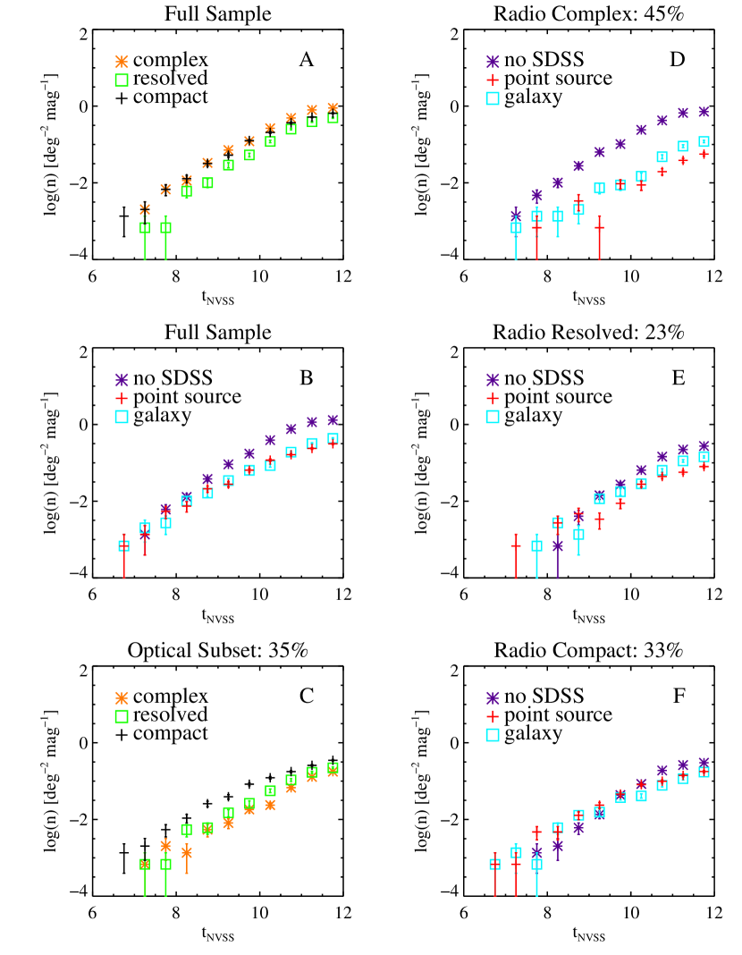
Figure 12: Magnitude distributions for sources detected by all four radio surveys. Panel A: Full sample divided by radio morphology. Panel B: Full sample divided by optical identification. Panel C: Optically-identified subset divided by radio morphology. Panels D-F: Complex, resolved, and compact radio sources, respectively.

Figure 12 shows $t_{\mathrm{NVSS}}$ magnitude distributions for sources detected by all four radio surveys and brighter than $t_{\mathrm{NVSS}}=12$, corresponding roughly to the GB6 detection limit (see §3.5). For the optically-matched subset, most sources have compact radio morphology, while the fraction of complex sources drops dramatically. This is partly due to the fact that radio-optical matched samples are biased against double-lobed sources (Lu et al., 2007). The fractions of sources in each morphology class remain roughly constant with $t_{\mathrm{NVSS}}$ even for the optically-matched subset. In all three radio morphology classes, galaxies and point sources are found in roughly equal ratios at all magnitudes.

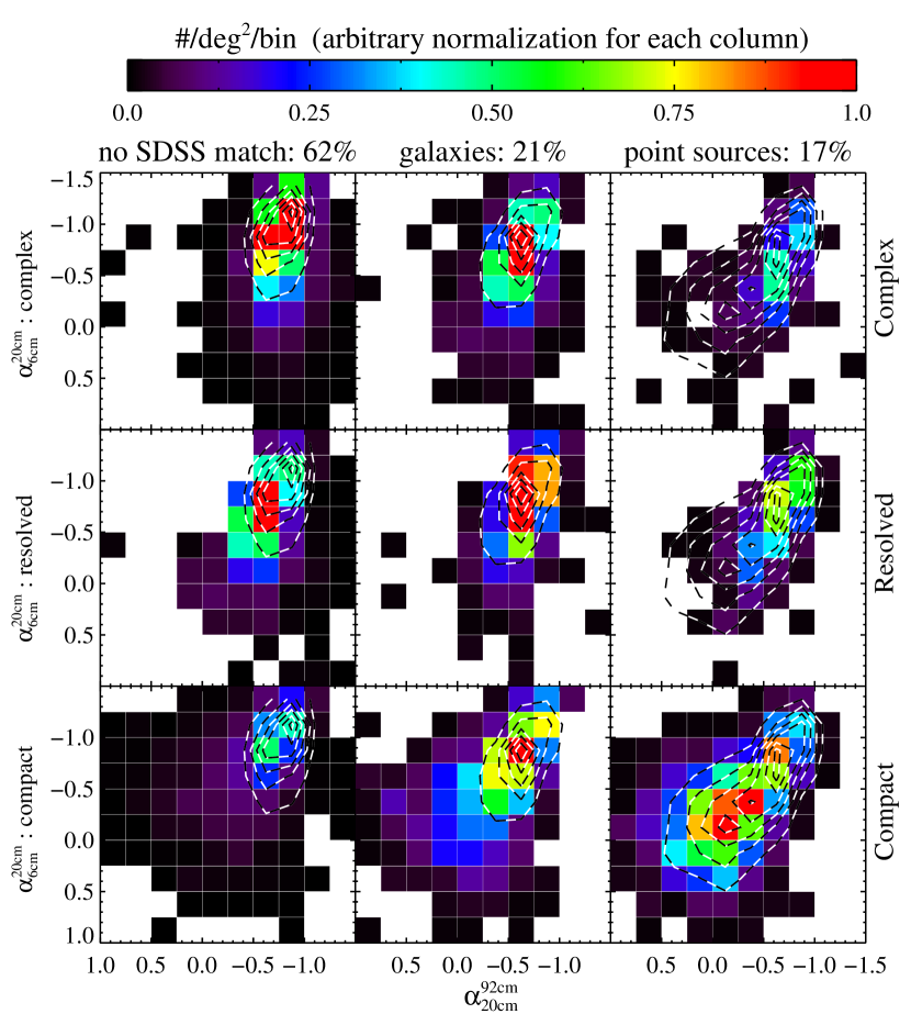
Figure 13: Radio color-color diagrams for sources detected by all four radio surveys divided into the nine radio/optical classes. The abcissa is $\alpha^{92}_{20}$; the ordinate is $\alpha^{20}_{6}$. From top to bottom, rows contain complex, resolved, and compact radio sources. From left to right the columns contain optically undetected sources, optically resolved sources, and optically unresolved sources. Contours in each column show the underlying distribution of all sources in the corresponding column. Contour levels and histogram normalization are arbitrary for each column.

Figure 13 shows radio color-color diagrams for the nine radio morphology/optical identification classes. This figure is an expansion of the middle column of Figure 10, with the addition of the three optical identification categories. Faint sources, galaxies, and point sources show different color-color distributions in the three morphology classes, particularly in the compact sample. For the complex sample, faint optical sources peak at steep values of $\alpha\sim-1$ while point sources peak near $\alpha\sim-0.5$. Galaxies are more tightly clustered around the peak than point sources. The sharpest separation in behavior is seen in the compact morphology sample (bottom row). The optically-faint and galaxy samples tend to have steep spectral indices ($\alpha<-0.5$), while point sources tend to have flat spectral indices ($\alpha>-0.5$). This confirms, with much improved statistics, the long-known distinction between flat spectrum radio quasars which are dominated by core emission and steep spectrum radio quasars which are dominated by lobe emission (Krolik, 1999). The compact point sources are also bimodal, with both a flat-spectrum and a steep-spectrum peak, while point sources in the complex and resolved morphology classes are primarily steep-spectrum. The steep-spectrum peak in the compact morphology class (lower right panel) may be due to distant, unresolved galaxies contaminating the point source sample.

The separation of the steep- and flat-spectrum peaks in color-color space is maximized along the $\alpha^{92}_{20}=\alpha^{20}_{6}$ locus. We thus take the average of the two indices to quantitatively investigate spectral slope distributions, as presented in Figure 14. Complex and radio resolved classes contain primarily steep spectrum sources, while the optically-identified radio compact sample is bimodal with a peak due to flat-spectrum point sources and a peak due to steep spectrum galaxies. The optically-faint subset of the compact morphology class is biased toward steep-spectrum sources (compare panels A and C). The distributions for the optically faint sample are similar to those of the galaxy sample. These histograms are based on the largest multi-wavelength samples of radio sources ever constructed. Table 5 compares the mean, median, and FWHM for the distributions in panels A, D, E, and F.

4.3.2 The NVSS-FIRST-WENSS sample

The majority of radio sources have $\alpha<-0.5$, i.e. they are brighter at longer radio wavelengths. The sample of sources detected by all four radio surveys is therefore flux limited by the short wavelength GB6 survey. Dropping the requirement of a detection in GB6 increases the number of selected sources to 64,000, a factor of five, while spectral slope information is still available from $\alpha^{92}_{20}$. The $\alpha^{92}_{20}$ distributions for the larger sample of NVSS-FIRST-WENSS detections (not shown) include much fainter sources; the observed bimodality seen in Figure 14 is still present, although the separation is weaker. Mean, median, and FWHM of the $\alpha^{92}_{20}$ distributions for the samples in Figure 14 are shown in Table 6. We use the NVSS-FIRST-WENSS subsample (listed as sample D in Appendix B) for all further data analysis.

4.3.3 Summary of source characteristics in the unified radio catalog

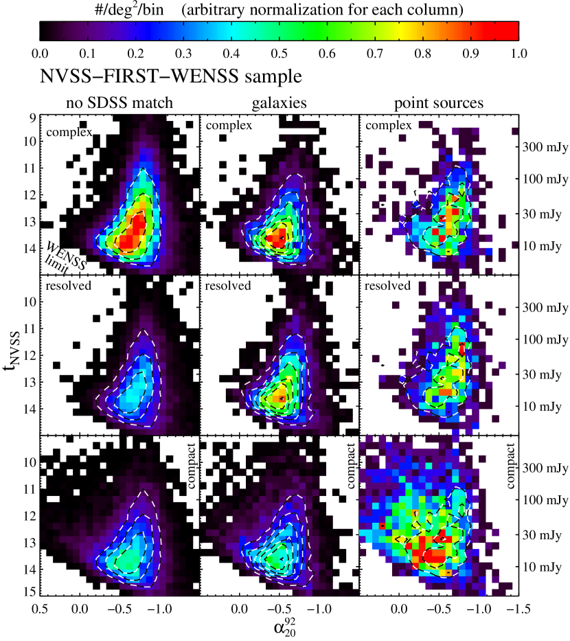
Figure 15: Radio color-magnitude diagrams for the nine radio/optical subclasses from the NVSS-FIRST-WENSS sample, categorized by radio morphology and optical identification. From top to bottom, the rows contain complex, resolved, and compact radio sources. From left to right, the columns contain the 46,517 optically undetected, the 12,780 optically resolved, and the 4,363 optically unresolved sources. The left axis is labeled with radio magnitude; the right axis with corresponding flux. Contours correspond to all the sources in each column; contour levels and histogram normalization are arbitrary for each column. Note that radio sources without an SDSS match are dominated by complex steep sources ($\alpha^{92}_{20}<-0.5$), while those matched to an SDSS point source are dominated by compact flat sources ($\alpha^{92}_{20}>-0.5$).

Figure 15 shows radio color-magnitude diagrams for NVSS-FIRST-WENSS sources from the catalog overlap region, providing a qualitative summary of fundamental properties of radio sources in the unified catalog. This figure expands the left panel of Figure 10 by adding classes defined by the optical identification categories. However, Figure 10 was limited to sources observed by GB6 in addition to NVSS, FIRST, and WENSS, resulting in a sample of only the brightest radio sources. Figure 15 demonstrates that GB6 detections are not necessary to obtain an extensive characterization of these radio sources, including radio spectral slope. Sources as faint as $t_{\mathrm{NVSS}}\approx 13.9$ can be studied without biasing toward steep-spectrum sources. The sample presented here contains 63,660 radio sources (optical subset: 18,728). Constraining to $t_{\mathrm{NVSS}}<13.9$ results in a sample of 50,046 (optical subset: 15,424). This catalog represents a significant increase in comprehensive radio data available to the scientific community.

Figure 15 provides a visualization of the unified radio catalog in a five dimensional parameter space defined by four radio magnitudes ($t_{\mathrm{NVSS}},t_{\mathrm{FIRST}}$ (integrated), and $t_{\mathrm{FIRST}}$ (peak) at 20 cm; $t_{\mathrm{WENSS}}$ at 92 cm) and one optical morphology parameter (optical light concentration; see §2.2.1). The four radio magnitudes are combined into parameters indicating magnitude, morphology, and spectral slope. Using three radio morphology classes, radio magnitude, spectral slope, and three optical identification/morphology subclasses, we have summarized the five-dimensional parameter space using the nine two-dimensional panels (radio color-magnitude diagrams) in this figure.

The marginal distributions of spectral index $\alpha^{92}_{20}$ for the sample in Figure 15 are similar to the distributions shown in Figure 14. However, the bimodality seen in the compact sample is reduced. This is due both to the inclusion of fainter sources, and the fact that one must use $\alpha^{92}_{20}$, rather than the average of $\alpha^{92}_{20}$ and $\alpha^{20}_{6}$, to describe the radio spectra of a sample that does not require detection at 6 cm.

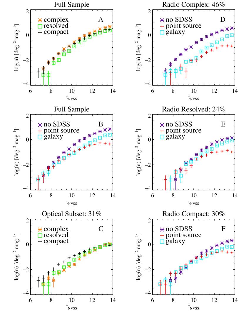
Figure 16: Magnitude distributions for sources detected by NVSS, FIRST, and WENSS. Panel A: Full sample divided by radio morphology. Panel B: Full sample divided by optical identification. Panel C: Optically-identified sources divided by radio morphology. Panels D-F: Complex, resolved, and compact radio sources, respectively, divided by optical identification.

Magnitude distributions for the nine radio/optical morphology subclasses are shown in Figure 16. This is the equivalent to Figure 12, but corresponding to the five times larger sample of NVSS-FIRST-WENSS sources. This figure shows the striking result that, at magnitudes fainter than $t_{\mathrm{NVSS}}=11.5$ ($\approx$100 mJy), the density of optical point sources flattens out dramatically, rather than continuing to rise as would be expected for a homogenous source distribution. This catalog is the first sample of radio sources both large and deep enough to investigate such faint source counts. The same behavior is seen in all morphology classes: point source counts flatten out while galaxy counts continue to rise at faint magnitudes.

4.4 Optical analysis aided by radio information

In the previous section, we showed that analysis in radio space is greatly aided by the addition of optical information. Similarly, the standard optical analysis, such as determination of optical luminosity function and its evolution with redshift, can benefit from the addition of radio observations. For example, one can ask whether radio loudness and radio spectral index correlate with optical quantities (e.g., “Can SDSS data alone predict the strength and spectral properties of radio emission?”). In this section, we take initial steps in this direction by examining the dependence of radio spectral slope on redshift and optical magnitude for quasars, and on optical magnitude and color for galaxies. We also investigate the relationship between radio loudness, radio spectral slope, and optical color.

We adopt the spectral index $\alpha^{92}_{i}$ as a measure of radio loudness, where

$$\alpha^{92}_{i}=0.0657(t_{\mathrm{WENSS}}-i).$$ (8)

This spectral index relates the 92 cm flux to the SDSS $i$ band flux, and can be converted to the often used radio loudness measure, $R_{i}=0.4(i-t_{\mathrm{FIRST}})$ (e.g. Ivezić et al., 2002) via

$$\alpha^{92}_{i}=0.11\alpha_{20}^{92}-0.16\,R_{i}.$$ (9)

A minimum in the radio loudness distribution at $R_{i}\sim 1$ reported by Ivezić et al. (2004b) corresponds to

$$\alpha^{92}_{i}=0.11\alpha_{20}^{92}-0.16\sim-0.25.$$ (10)

The NVSS-FIRST-WENSS sample analyzed here is not sufficiently sensitive to investigate radio loudness bimodality, due to the WENSS flux limit.

Throughout this section, we focus on sources observed by the NVSS, FIRST, WENSS, and SDSS surveys, with optical spectra from the SDSS. We assume a cosmology with $H_{\mathrm{0}}=70~{}\mathrm{km~{}s}^{-1}\mathrm{Mpc}^{-1}$, $\Omega_{M}=0.3$, and $\Omega_{\Lambda}=0.7$.

4.4.1 Spectroscopically-identified quasars

To find a sample of spectroscopically-identified radio quasars, we match unified catalog sources to the Fifth Data Release (DR5) SDSS Quasar Catalog (Schneider et al., 2007, hereafter S07). This catalog is a cleaner quasar sample than sources identified as quasars by the SDSS spectroscopic software pipeline: the S07 spectra have been visually examined to verify that they have at least one broad emission line (FWHM $\gtrsim 1000~{}\mathrm{km~{}s}^{-1}$) or are unambiguously broadline quasars. Candidates for the visual examination included all sources selected by the SDSS quasar target selection algorithm, and all sources identified as quasars after spectroscopic observation.

The sample used here consists of the 1,288 NVSS-FIRST-WENSS sources matched to an S07 source within $2\arcsec$ (sample H). Note that because the quasars were discovered via various SDSS target selection algorithms, they do not represent a complete statistical dataset. Indeed, proximity to a FIRST source is one of the selection methods. One therefore must be careful when creating statistical samples from this data set; e.g. one must choose quasars identified by the same target method, and account for sources in regions of the sky where different target selections were used. Note however that the SDSS optical quasar sample is estimated to be complete at the 94.6% level for the magnitude range $16<i<19.$ and redshifts less than 5.8 (Richards et al., 2002).

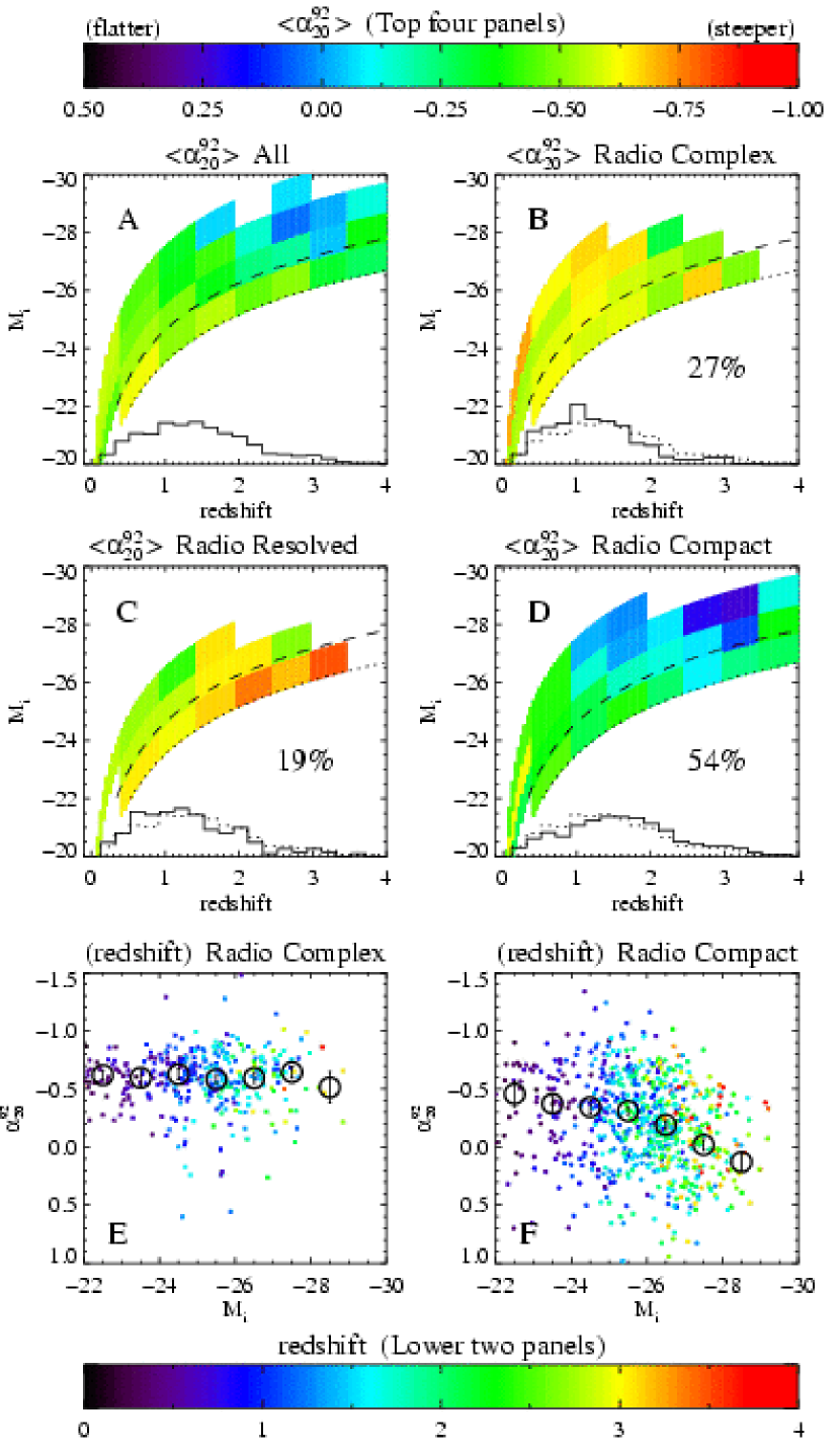
Figure 17: Distributions in absolute magnitude-redshift-spectral index parameter space for the spectroscopic quasar sample. The dotted and dashed lines indicate the $i<20.2$ and $i<19.1$ limits, respectively, used in the quasar target selection algorithm. Panel A: absolute magnitude vs. redshift for the full sample, with bins in redshift and apparent magnitude color-coded by the median value of $\alpha^{92}_{20}$ (upper colorbar). The histogram at the bottom of the panel shows the redshift distribution. Panels B through D: panel A divided into the three radio morphology subclasses. The percentage of quasars in each morphology class is given. Full histograms show the redshift distribution in each panel; for comparision the redshift distribution of the full quasar sample is also shown (dotted line). Histograms have been normalized such that all have equal area. Panels E and F: Spectral index vs. optical absolute magnitude distributions for complex and compact radio sources, respectively. Points are color-coded by redshift. Circles show the median value of $\alpha^{92}_{20}$ in bins of 1 magnitude.

Figure 17 investigates the dependence of radio spectral slope on optical luminosity and redshift for quasars with different radio morphologies. Optical K-corrections used to calculate absolute magnitude $M_{i}$ assume an optical spectral index $\alpha=-0.5$ (Ivezić et al., 2002). Panel A shows that the radio spectral slope for radio quasars is independent of redshift and is a strong function of absolute magnitude: quasars with the steepest radio spectra tend to be optically faint. We investigate this correlation as a function of radio morphology in panels B-D: the trend is seen quite strongly in the compact morphology class, but is weak for the complex and resolved sources. Additionally, compact quasars have the flattest radio spectra, while radio spectra of complex sources are relatively steep.

A more quantitative visualization of the correlation between radio spectral slope and optical luminosity is shown in Panels E and F, for radio complex and radio compact sources, respectively. The median value in unit magnitude bins is indicated by black circles. The median spectral slope for complex sources is constant with luminosity, while the median slope for compact sources is a strong function of luminosity. This trend may indicate a physical change in radio spectral slope with optical luminosity, an orientation effect, and/or intrinsic variation in spectral slope combined with luminous sources being observed at higher redshifts (i.e., a radio K-correction effect). Figure 18 shows as an example a simulated spectrum that steepens for $\lambda>20$ cm, which would show the observed trend when viewed at different redshifts. It has been suggested however that spectral slope is an indication of orientation (Jarvis & McLure, 2006), and therefore of increased Doppler beaming. The spectrum of a quasar viewed along a line of sight close to the jet axis is highly core-dominated. It would thus appear flatter than a source viewed off-axis, while beaming would lead to a higher observed luminosity. Complex sources (Panel E) can be expected not to show the same trend, as they almost certainly have extended emission from steep-spectrum radio lobes, biasing against sources with strongly-beamed jets. On the other hand, the compact sample may contain unresolved core-lobe sources, especially at higher redshift. An angular size of $5\arcsec$ (FIRST resolution) corresponds to $\sim 40$ kpc at redshift 1. According to Blundell & Rawlings (2000, Fig. 2), a typical quasar can reach this size in $\sim 10^{6}-10^{7}$ years while the maximum active lifetime is estimated to be $10^{8}-10^{9}$ years. However, a line-of-sight alignment near the jet axis would significantly shorten the projected linear size, decreasing the likelihood of resolving a core-lobe source. Note that the combination of a flat core component and a steep lobe component can result in a spectrum of the type shown in Figure 18. The trend observed in Panel F may therefore be due to an intertwined, and inseparable, combination of the above effects.

Equivalent plots to Panels E and F (not shown) indicate that the median value of $\alpha^{20}_{6}$ at all optical luminosities corresponds to a flat spectrum between 6 and 20 cm in all three morphology classes, which lends support to the K-correction argument. There are quasars whose spectra are consistent with the simulated example shown in Figure 18, but not all, as demonstrated in Fig. 2 of Kuehr et al. (1981). However, the resolution of their observations was very low. To accurately determine the radio spectral shape of quasars will require better frequency resolution, which will be possible with the future Expanded VLA project (Napier, 2006).

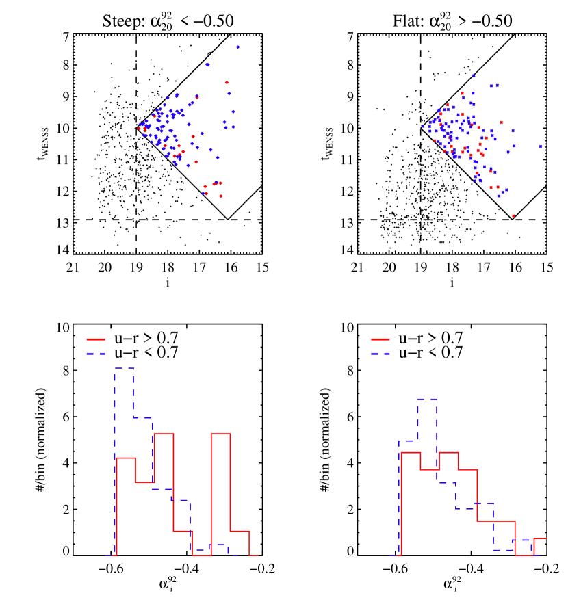
Figure 19: Distribution of $\alpha^{92}_{i}$, a measure of radio loudness, for the spectroscopic quasar sample. The top two panels show the region of radio magnitude-optical magnitude space selected so as not to bias toward radio quiet or radio loud sources. The lower two panels show $\alpha^{92}_{i}$ histograms for red ($u-r>0.7$; solid line) and blue ($u-r<0.7$; dashed line) quasars. The left panels correspond to sources with steep radio spectra; panels on the right correspond to sources with flat radio spectra.

The dependence of radio loudness on radio spectral slope and optical color for quasars is investigated in Figure 19. Sources are divided into steep- (left) and flat-spectrum (right). We require $t_{\mathrm{WENSS}}<12.9$ so as not to bias against any sources with $\alpha^{92}_{20}\gtrsim-1.5$. We require $i<19$ to ensure a complete sample of quasars. Based on those two limits, we have selected a region of radio/optical magnitude space which does not bias against radio quiet or radio loud sources (top two panels). The radio loudness distribution of steep-spectrum quasars (lower left panel) is strongly dependent on color: a Kolmogorov-Smirnov test rejects the null hypothesis that the two histograms share the same parent distribution at the 99.6% level. No such dependence is seen for the flat-spectrum quasars (lower right panel). This paper presents the first observation of this effect. Note that the requirement of a detection at 92 cm biases these samples to bright radio fluxes, and prevents us from reaching the expected local minimum in the $\alpha^{92}_{i}$ distribution at $\alpha^{92}_{i}\sim-0.25$.

4.4.2 Spectroscopically-identified galaxies

The sample of spectroscopically-identified galaxies (sample G) is the set of 2,885 NVSS-FIRST-WENSS-SDSS matches whose spectra identify them as galaxies, according to the SDSS automatic classification software. Here, we restrict our analysis to a flux-limited sample with $r<17.77$, in order to choose galaxies from the SDSS main galaxy sample (Strauss et al., 2002). The resulting flux-limited sample consists of 1,656 spectroscopic galaxies.

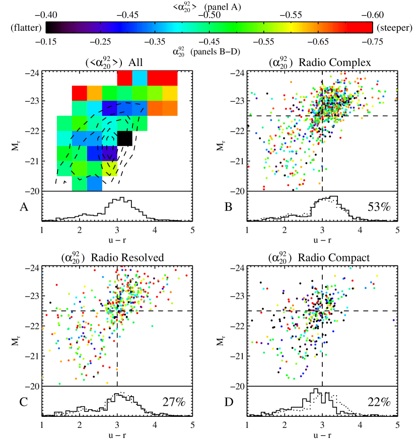
Figure 20: Distribution in color, magnitude, spectral index parameter space for the flux-limited ($r<17.77$) spectroscopic galaxy sample. Panel A: Color-magnitude diagram for the full sample with bins color-coded by the median value of $\alpha^{92}_{20}$. Contours show the distribution of all $r<17.77$ SDSS spectroscopic galaxies. The histogram below shows the $u-r$ distribution. Panels B through D: panel A divided into the three radio morphology classes, as labeled. Points are color-coded by $\alpha^{92}_{20}$. Percentage of galaxies in the subclass is given in the lower right corner. Dashed lines at $u-r=3$ and $M_{r}=-22.5$ are provided to guide the eye. The histogram underneath shows the $u-r$ distribution (solid line), compared to the distribution for the full sample (dotted line; equivalent to solid line histogram in Panel A).

Figure 20 investigates the dependence of radio spectral slope on optical luminosity and color for galaxies. Complex galaxies tend to have steeper radio slopes than compact galaxies. Radio sources with flat spectrum emission are generally understood to be quasar cores (i.e., quasar sources without radio lobes, Krolik, 1999). Quasar core sources are compact in the radio due to their small size and typically large distances. Sources in panel D therefore beg the question: what are the flat-spectrum, radio compact sources that are optically-identified as galaxies? It is possible that those sources are quasars too weak in the optical to overpower emission from the galaxy, observed as galaxies with AGN (e.g. Seyfert galaxies, LINERS), a possibility we will investigate in future work.

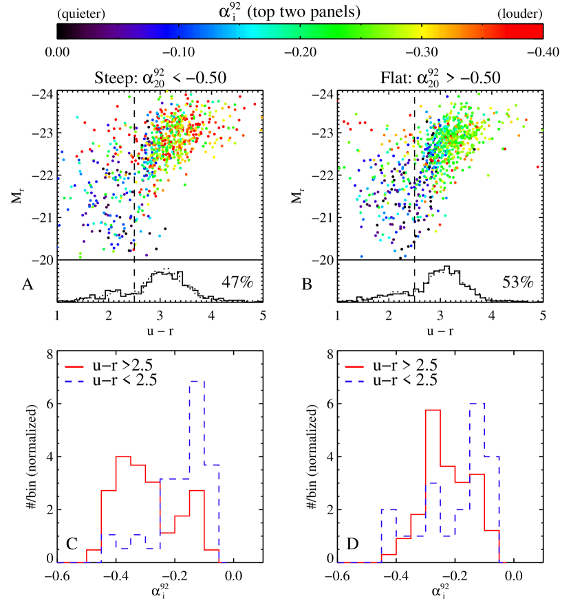
Figure 21: Distributions in color, magnitude, and radio to optical spectral slope for the flux-limited ($r<17.77$) spectroscopic galaxy sample. Panels A and B: Color-magnitude diagrams ($M_{r}$ vs. $u-r$) for steep- and flat-spectrum radio sources, respectively; points are color-coded by the radio to optical spectral slope ($\alpha^{92}_{i}$). The solid line histogram shows the $u-r$ distribution; the dotted line histogram shows the $u-r$ distribution of the full sample (equivalent to solid line histogram in Panel A of Figure 20). The dashed vertical line indicates $u-r=2.5$. The percentage of galaxies in each class is given in the lower right corner. Panels C and D: Normalized distributions of $\alpha^{92}_{i}$ for red ($u-r>2.5$) and blue ($u-r<2.5$) radio galaxies from the top two panels.

Figure 21 explores the dependence of radio loudness of galaxies on optical luminosity and color. The top row shows the distribution of steep- (left) and flat-spectrum (right) sources in optical color-magnitude diagrams with points color-coded by $\alpha^{92}_{i}$. Note that only very luminous galaxies are radio loud ($\alpha^{92}_{i}\lesssim-0.35$ for $M_{r}<-22$). The lower two panels show the distribution of $\alpha^{92}_{~{}i}$ for steep and flat radio galaxies divided by $u-r$ color. Similar to Fig. 19, we focus on an unbiased region of radio/optical magnitude space, based on the limits $t_{\mathrm{WENSS}}<12.9$ and $i<17$. The lower left panel shows a significant difference in radio loudness for blue (dashed line) and red (solid line) steep-spectrum radio galaxies. The blue galaxies have a median $\alpha^{92}_{i}$ of $\sim-0.13$, while the median value for red galaxies is $\sim-0.26$. A difference of 0.13 in $\alpha^{92}_{i}$ (Eq. 8) corresponds to a change of about 2 magnitudes, i.e. steep-spectrum red galaxies are about two orders of magnitude brighter in the radio than steep-spectrum blue galaxies of the same optical brightness. The distributions of radio loudness for blue and red flat-spectrum galaxies are not significantly different.

5 CATALOG APPLICATIONS/FUTURE WORK

The information provided by this catalog will enable many diverse studies. In this section, we briefly remark on applications toward the investigation of the radio quasar/galaxy unification theory, the search for radio stars, and the selection of possible high-redshift galaxies. We then describe the usefulness of the catalog for studies of the evolution of the radio universe by comparison with models, which we discuss in detail in a companion paper (A. Kimball et al. in preparation).

5.1 Unification paradigm for radio-loud active galactic nuclei

The orientation-based unification scenario (Urry & Padovani, 1995) was originally motivated by the similarity of radio emission from sources that appear very different optically, i.e. quasars and galaxies. The theory assumes that sources whose emission is dominated by a radio core or lobes are members of the same “parent” population, but differ in appearance because their highly anisotropic emission is viewed from different angles. This anisotropy is predominantly due to relativistic motion of the plasma in the inner jets and Doppler boosting (“beaming”) when the angle between the line of sight and the plasma velocity vector is small (Krolik, 1999). Hence, the same object could appear as a core source when viewed at small angles (with the “boosted” core outshining the lobes), and as an extended double-lobe or a core-lobe source otherwise. Understanding the radiation anisotropies in AGNs is required to unify the different types; that is, to identify each single, underlying AGN type that gives rise to different observed classes through different orientations (Antonucci, 1993; Urry & Padovani, 1995).

The unified catalog allows users to classify many quasars and galaxies according to their radio morphology (e.g., core sources, lobe sources) and spectral behavior. Statistical studies of such objects will lend evidence for or against the unification paradigm by the investigation of number statistics, the size versus orientation distribution, and environment. The unification scenario has successfully explained many observed properties of bright radio sources in previous research (Barthel, 1989; Urry et al., 1991; Padovani & Urry, 1992; Lister et al., 1994; Urry & Padovani, 1995), but recent studies suggest there may be some intrinsic differences between radio quasars and galaxies (Willott et al., 2002).

5.2 A method for selecting high-redshift ($z>1$) galaxy candidates

Galaxies at high redshift are important for studies of large scale structure and galaxy evolution, and in fact the higher the redshift of a galaxy the more useful it is for these studies. Candidate high-redshift galaxies can be selected from the unified catalog based on their radio morphology, radio spectral slope, and lack of an optical counterpart. The lack of optical counterpart requirement is intended to select sources so distant that their observed optical emission lies blueward of the rest-frame $4000$Å break (e.g., Madau et al., 1996). As the optical sources used herein were selected in the $r$ and $i$ bands at 6165Å and 7481Å respectively, this requirement will tend to select galaxies at redshifts of $z\sim 1$ and higher. A steep radio spectrum has often been used as a criterion to find high-redshift sources, owing to the fact that higher redshift objects are observed at higher rest-frame frequencies, and because radio galaxy spectra tend to flatten below $\sim 300$ MHz in their rest frame (e.g., Cruz et al., 2006, and references therein). Additionally, as discussed in §4.3, in the compact morphology subclass a steep radio spectrum is a likely indicator of an optically-resolved source.

To find a sample of candidate high-redshift galaxies, we select sources which are unresolved by FIRST, undetected by the SDSS, and have steep radio spectra. Specifically, we begin with the sample of objects identified by NVSS, FIRST, and WENSS which have compact radio morphology. We require $\alpha^{92}_{20}<-0.5$ and no SDSS match within $3\arcsec$. Note that heavily dust-obscured galaxies are also likely to be found in such a sample. In the catalog overlap region, the above criteria select 9,953 sources. Visual examination of SDSS images of all the candidates revealed 334 suspect sources, i.e. radio positions coinciding with a diffraction spike, scattered light, a nearby star or galaxy, etc. Removing the suspicious sources results in a sample of 9,619 candidate $z>1$ galaxies. It will be interesting to compare this sample with deeper optical surveys and observations at other wavelengths, as the data become available. This sample is available for download on the catalog website (sample K).

5.3 The search for radio stars

With the great increase in the sensitivity of radio surveys in the last several decades, along with the more accurate source positions afforded by radio interferometry, comes the ability to search for fainter and rarer radio sources. A small fraction of stars have significant non-thermal radio emission, such as dMe flare stars (White et al., 1989) and cataclysmic variables (Chanmugam, 1987; Mason & Gray, 2007), but most stars have only weak thermal radio emission. Because quasars and stars lie in different locations in SDSS color-color diagrams (Ivezić et al., 2002; Richards et al., 2001), it may be possible to select a clean sample of radio stars based on their photometric colors. To investigate this possibility, we select a sample of radio star candidates from the unified radio catalog.

We begin by selecting point sources from the catalog overlap region which coincide with a FIRST radio detection. We use a conservative matching distance of $1\arcsec$ to limit the contamination due to random matches. To ensure a sample for which the majority have spectra, we require $i<19$. We eliminate the region of color-color space where quasars are commonly found: $u-g<0.8$ and $-0.2<g-r<0.6$.

The number of candidates remaining after each step of the selection algorithm is shown in Table 7. The resulting sample of 532 candidate radio stars contains 406 objects with SDSS spectra. From the SDSS spectral classifications, we determine that 78 are stars, 313 are quasars, and 15 are galaxies. The results of applying the selection to the SDSS DR5 quasar catalog (Schneider et al., 2007) are also shown for comparison. The completeness of the quasar catalog is $\sim 95\%$ (Richards et al., 2002; Vanden Berk et al., 2005). Seven of the known quasars were identified as galaxies by the SDSS spectroscopic pipeline, and two as stars. The latter are actually the super-position of a star and a quasar: the spectra are primarily stellar, but also contain at least one broad emission line. Note that 33 of the candidate radio sources classified as “quasar” are absent from the quasar catalog. These are sources that were spectrocopically-observed for the sixth SDSS data release, but are not in DR5.

The sky density of unresolved $i<19$ SDSS sources is $\sim 1000\deg^{-2}$, while the density of quasars is $\sim 10\deg^{-2}$. However, out of nearly 6 million point sources with $i<19$, we found only 78 confirmed radio stars, implying that the likelihood of a star being a radio source is approximately $10^{-5}$, while the likelihood for a quasar is about $8\times 10^{-2}$. Consequently, despite using a conservative color cut to eliminate probable quasars, the sample is dominated by radio quasars rather than radio stars. Using this color-color selection is therefore not an efficient way to find radio stars. One must have spectral classification in order to select a clean radio star sample; photometric observations alone are not sufficient.

5.4 Radio galaxy evolution models

In the companion paper, we attempt to understand and quantitatively explain the observed source counts for the nine subclasses defined by radio morphology and optical identification (Fig. 13), with the aid of models. Barai & Wiita (2006, 2007) investigated a large number of input parameter variations for several radio galaxy evolution models and compared the resulting distributions of radio power, spectral index, linear size, and redshift to the low-frequency ($\sim$2 m) Cambridge catalogs (Laing et al., 1983; Eales, 1985; McGilchrist et al., 1990). They found that none of the models was able to provide good simultaneous fits to all observables for all three catalogs, but noted that the observational datasets were too small to adequately constrain the model parameters.

The catalog presented in this paper represents a significant increase in the size of radio samples for which luminosity, size, spectral slope, and redshift can be measured. We will compare the observed distributions from the unified catalog to distributions of sources from mock catalogs (obtained by applying observational selection criteria to the computer-generated radio skies). The distributions will help to constrain the increasingly sophisticated models of radio galaxy evolution. The models will thus help explain the physics and evolution leading to the distributions seen in the unified catalog.

5.4.1 Defining a long-wavelength flux-limited sample

The radio galaxy evolution models currently perform best at long wavelengths, where emission is dominated by the radio lobes. The most robust approach for comparing models and observations is therefore to define a flux-limited sample using long-wavelength measurements, such as the 92 cm flux from the WENSS survey. Fortunately, because most radio sources are brighter at longer radio wavelengths, a source observed in WENSS (faint limit of 18 mJy) is almost guaranteed to be detected at 20 cm (faint limits of 1 mJy for FIRST and 2.5 mJy for NVSS). However, the 92 cm flux limit must be chosen carefully in order to avoid biasing against sources with radio spectra so steep that they are too faint at 20 cm to be detected by NVSS. The color-magnitude diagrams and spectral slope histograms presented in the data analysis of this paper indicate that very few radio sources have a spectral slope index less than -1.5 between 20 and 92 cm. To ensure an NVSS detection for all sources with $\alpha^{92}_{20}<-1.5$ in a flux-limited sample requires $t_{\mathrm{WENSS}}\leq 12.9$ (see Eq. 7). We positionally matched all $t_{\mathrm{WENSS}}<12.9$ sources in the WENSS survey to NVSS and FIRST, and found that only 1% did not have a match in NVSS. We interpret this value as an upper limit on the fraction of sources with $\alpha^{92}_{20}<-1.5$. Ninety-five per cent of the WENSS sources have both a FIRST detection and an NVSS detection within $30\arcsec$. The sample of NVSS-FIRST-WENSS matches with $t_{\mathrm{WENSS}}<12.9$ in the unified catalog contains 47,567 sources. Over 12,000 of those have optical counterparts, from which a cosmological distance can be determined via photometric redshift techniques. Photometric redshifts from the SDSS are accurate to $\sim 0.06$ for luminous red galaxies with redshifts $z<0.7$ (Padmanabhan et al., 2005). A further 3,000 of the radio-optical sample additionally have SDSS spectroscopic redshifts. This dataset therefore represents a major size increase compared to the sample of 327 sources used by Barai & Wiita.

6 SUMMARY

We have presented a unified catalog of radio objects by combining observations from several radio and optical surveys. The complete catalog is available online, along with scientifically useful data subsets. Using several parameters determined from the measured radio fluxes, we investigated the distribution of sources in radio color-magnitude-morphology space and optical color-redshift-luminosity space.

To create the catalog, we merged together the two 20 cm radio surveys, FIRST and NVSS. Included are FIRST-NVSS associations (three sources from each survey with the closest proximity to sources in the other survey, within $30\arcsec$), FIRST sources with no NVSS counterpart, and NVSS sources without a nearby FIRST counterpart. Where sources had a counterpart in one of the other three surveys, we supplemented the catalog data with 6 cm, 92 cm, and optical observations.

For a preliminary data analysis, we converted the radio fluxes (6 cm, peak 20 cm, high- and low-resolution integrated 20 cm, and 92 cm) into several useful parameters describing 20 cm radio magnitude, 20 cm radio morphology, radio spectral slope, and optical identification/luminosity. The automatic morphology classification divides sources into “complex”, “resolved”, and “compact” categories, with results that compare well to visual morphology classification. Using various radio color-magnitude diagrams, we found that most radio sources have a steep radio spectral slope between 6 and 20 cm ($\alpha\sim-0.8$, where $F_{\nu}\propto\nu^{\alpha}$). However, the radio compact sources contain a significant fraction of flat-spectrum sources ($\alpha\sim 0$). SDSS morphological identifications for optically-matched sources indicate that the steep-spectrum compact sources are primarily galaxies, while flat-spectrum compact sources are primarily optically unresolved (i.e., quasars). The complex and radio resolved sources contain comparable numbers of both galaxies and optical point sources.

Focusing on sources with SDSS spectra, we investigated the dependence of radio spectral slope and radio loudness on optical quantities (color, magnitude, redshift) for quasars and galaxies. For complex and radio resolved quasars, no significant dependence of spectral slope on redshift or optical magnitude was found. For compact quasars, however, radio spectral slope seems to flatten out with increasing redshift/luminosity. The trend is consistent with a radio K-correction resulting from a spectrum that is steep at wavelengths longer than 20 cm and flat for wavelengths shorter than 20 cm, but may also be an effect of orientation and Doppler beaming. Formally, a Kolmogorov-Smirnov test showed a dependence on optical color for the radio loudness distribution of steep-spectrum quasars. No color-dependence was found for the flat-spectrum quasars. In the galaxy sample, the compact morphology class tends to be bluer and fainter, with flatter radio slopes, than either the complex or radio resolved class. Among steep-radio-spectrum galaxies, the red sources have radio fluxes on average two orders of magnitude brighter than the blue sample.

We have presented methods for selecting candidate radio stars and candidate high-redshift galaxies from the unified catalog. We concluded that a conservative color-selection attempting to reduce contamination from quasars still yields a sample that is completely dominated by quasars rather than radio stars. Spectra are therefore necessary to successfully identify radio stars.

In a companion paper (A. Kimball et al. in preparation), we will compare the results of several state-of-the-art models for radio galaxy evolution to observations yielded by the unified catalog, and test the unification paradigm for powerful radio galaxies and quasars.

While this is not the first catalog to combine observations in the radio and the optical to further the study of radio galaxies and radio quasars, the unified catalog presented in this paper has significant advantages over previous studies. It is the largest catalog to date that combines optical observations with multi-wavelength radio data. It can be used to define a long-wavelength (92 cm) flux-limited sample of nearly 50,000 sources detected in WENSS, FIRST, and NVSS. Comparing 20 cm FIRST and NVSS fluxes allows us to place every one of those sources into one of the three radio morphology classes, and the additional 92 cm detection allows us to calculate a radio spectral slope. Over one quarter of the long-wavelength flux-limited sample has an optical detection in the SDSS, including over 3,000 with spectra. The usefulness of the catalog will increase as larger surveys at different wavelengths with deeper observations become available. For example, the deep observations planned for the future Large Synoptic Survey Telescope will provide a nearly 100% optical identification rate, and extremely accurate photometry in six bands.

Appendix A CATALOG MATCHING

A.1 Matching FIRST and NVSS

In this section, we describe in detail the process of matching sources in FIRST and NVSS, and present a method for selecting a clean sample of 20 cm sources.

Before proceeding, it is necessary to define certain clarifying terms, some of which are data parameters found in the catalog. Our matching algorithm used a primary survey and a secondary survey. Source positions in the primary survey were used as search centers, and neighbors within a certain radius were found in the secondary survey. To find catalog sources we applied the matching algorithm twice: with FIRST as primary and NVSS as secondary, and again with NVSS as primary and FIRST as secondary. Each time, the three closest neighbors from the secondary survey were ranked by proximity to the primary source (within the pre-determined search radius). The advantage of performing the matching twice is that we can recover the three closest FIRST detections to a NVSS primary, and vice-versa. Each catalog row contains records for a single NVSS source and a single FIRST source. For an entry with an NVSS primary, the parameter matchflag_nvss is set to $-1$, while matchflag_first is set either to 0, indicating a primary source with no FIRST match, or to 1, 2, or 3 indicating the proximity ranking of the FIRST match. Conversely, for FIRST primaries matchflag_first is set to $-1$, and matchflag_nvss equals 0, 1, 2, or 3. Note that a single source can appear as the primary object in as many as three separate catalog entries.

Due to the lower spatial resolution and higher flux limit of NVSS, individual NVSS sources can be resolved into separate components by FIRST. Therefore, multiple FIRST detections matched to the same NVSS primary are common, while multiple NVSS detections matched to the same FIRST primary are rare. Figure 22 gives a visual example of common types of objects found in the catalog. FIRST sources are shown as small squares and NVSS sources as large circles. In quadrant A, an unresolved NVSS source is resolved into three components in FIRST (example: a radio quasar with two lobes); a fourth FIRST detection lies nearby. When taking FIRST as the primary survey, each of the four FIRST sources would identify the NVSS object as the nearest neighbor. When taking NVSS as the primary survey, the three closest FIRST sources would match to the NVSS source while the fourth would not. The NVSS source in Quadrant A would appear in seven catalog entries. It would appear in four rows with matchflag_first $=-1$ and matchflag_nvss = 1. It would appear in three rows with matchflag_nvss $=-1$ and matchflag_first = 1, 2, or 3. To cull out the duplicates in order to select a clean sample, one would simply require matchflag_nvss $=-1$ and matchflag_first $=1$.

The remaining objects in Figure 22 are simpler to match. Quadrant B contains a simple, isolated source identified by both surveys (examples: a radio quasar with no jets or a distant galaxy). Such an object would appear in two catalog rows: once with matchflag_first $=-1$ and matchflag_nvss = 1, and a second time with matchflag_nvss $=-1$ and matchflag_first = 1. Quadrant C contains a FIRST source without a NVSS counterpart (e.g., an object too faint to be detected by the latter); it would appear once in the catalog, with matchflag_first $=-1$ and matchflag_nvss = 0. In Quadrant D is a NVSS source unmatched by FIRST (e.g., a low surface-brightness galaxy). This source’s single catalog entry would have matchflag_nvss $=-1$ and matchflag_first = 0.

To find all sources detected by both surveys while minimizing duplicates, the simplest selection is to require matchflag_nvss $=-1$ and matchflag_first = 1. The resulting data set consists of 142,622 sources in the overlap region, with only 158 (0.11%) duplicate NVSS sources matched to the same FIRST source. Specific examples of data selections are given in Appendix B.

A.2 Matching to the SDSS

To match to the SDSS photometric catalog, we implemented a different technique from that used in matching the radio surveys. The motivation was to find the nearest neighbor, as well as the brightest neighbor within a pre-defined distance $D$, where $D$ was adjusted according to the distance of the nearest neighbor. We began by finding the nearest optical neighbor within $60\arcsec$ of each catalog entry. Where the distance $d_{near}$ to the nearest neighbor was less than $3\arcsec$, we defined $D=3\arcsec$. For $3\arcsec<d_{near}<10\arcsec$, we defined $D=10\arcsec$, for $10\arcsec<d_{near}<30\arcsec$ we defined $D=30\arcsec$, and for $30\arcsec<d_{near}<60\arcsec$ we defined $D=60\arcsec$. We then recorded the brightest neighbor within distance $D$. Each catalog entry contains two sets of data parameters corresponding to SDSS photometric matches: one set is identified by the prefix “near” and the other by the prefix “bright” (e.g. “near_modelmag_u”, “bright_modelmag_u”). Thirty-five per cent of FIRST sources in the overlap region have an SDSS counterpart within $3\arcsec$, 61% within $10\arcsec$, and over 98% within $30\arcsec$. In 98.8% of cases where an optical match was found within $3\arcsec$, the brightest and the nearest SDSS objects within $3\arcsec$ are the same.

Appendix B SELECTING DATA SAMPLES

In this section, we define in detail the samples described in this paper, and present several scientifically-useful data subsets available for download on the catalog website. Samples described in this appendix but not available online can be assembled from the complete catalog using the selection requirements given here.

Table 8 presents a summary of the data sets and their selection requirements. The meanings of catalog parameters referenced in the table (in italics) are as follows. Parameters ra and dec are right ascension and declination, respectively, in decimal degrees. Overlap indicates a source inside (value 1) or outside (value 0) the catalog overlap region. Matchflag_nvss and matchflag_first are set to $-1$ to indicate primary source catalog, 0 to indicate an isolated source, or 1, 2, 3 to rank matched source by proximity to primary source (see Appendix A for details). Distance indicates separation between FIRST and NVSS neighbors, in arcseconds. First_id, wenss_id and gb6_id are unique identifiers for the FIRST, WENSS and GB6 sources, respectively. Wenss_distance and gb6_distance indicate separation, in arcseconds, between WENSS or GB6 neighbors and the 20 cm source. Near_distance and near_type indicate respectively the distance to and object type of the nearest neighbor in the SDSS photometric survey, while spec_type indicates the SDSS spectral classification for objects from the spectroscopic survey. Matchtot30 indicates the number of neighbors within $30\arcsec$ of the primary 20 cm survey source (where neighbors come from the secondary 20 cm survey). For a full description of all 117 catalog parameters, we refer the reader to the catalog website.

B.1 Data sets discussed in the paper

The data samples discussed in this paper consist of sources detected by both FIRST and NVSS, sources detected by the three largest radio surveys (FIRST, NVSS, WENSS), sources detected by all four radio surveys (FIRST, NVSS, WENSS, GB6), and sources detected by all four radio surveys as well as the SDSS. Spectroscopic galaxy and quasar samples are created from the FIRST-NVSS-WENSS sources.

Sources detected by both FIRST and NVSS, matched within $25\arcsec$, are listed as sample C in Table 8. An efficient way of finding these pairs while culling duplicates is to select NVSS sources, and their nearest FIRST neighbor. These sources can be selected by requiring overlap = 1, matchflag_nvss =$-1$, matchflag_first = 1, and distance $\leq 25$. The resulting sample contains 141,881 objects ($48\deg^{-2}$) detected by both 20 cm surveys, which can therefore be classified by radio morphology.

Sample D contains sources detected by FIRST, NVSS, and WENSS. This is the subset of sample C with a WENSS counterpart within $30\arcsec$. Additional requirements to select this data set are wenss_id $\neq 0$ and wenss_distance $\leq 30$. The resulting sample contains 63,660 sources ($21.5\deg^{-2}$). These sources have three 20 cm fluxes and a 92 cm flux measurement, and can therefore be categorized by both radio morphology and spectral slope ($\alpha^{92}_{20}$).

Sample E contains sources detected by all four radio surveys; it is the subset of sample D that has a GB6 counterpart within $70\arcsec$. Selecting these sources requires additional parameter settings gb6_id $\neq 0$ and gb6_distance $\leq 70$. The sample is comprised of 12,414 sources ($4.2\deg^{-2}$), which can be categorized by radio morphology and two spectral slope measures.

Sample F contains sources detected by all four radio surveys and the SDSS. To select these sources from sample E requires near_type $\neq 0$ and near_distance $\leq 2$. The sample contains 4,732 sources ($1.6\deg^{-2}$), which can be categorized by radio morphology and two spectral slope measures, and identified as galaxies or point sources.

Sample G contains spectroscopically-identified galaxies detected by NVSS, FIRST, WENSS, and SDSS. These sources are a subset of Sample D, requiring spec_type = 2 and near_distance $\leq 2$. It contains 2,885 galaxies. Note that in §4.4.2, we restricted our analysis to a smaller, flux-limited sample of 1,656 spectroscopic galaxies with $r<17.77$.

Defining the spectroscopic quasar sample was more complicated than defining the spectroscopic galaxy sample. As discussed in §2.2.2, the quasar catalog of Schneider et al. (2007) is cleaner and hence more reliable than the set of spectroscopically-identified quasars supplied by SDSS DR6. To identify radio quasars with spectra, we therefore opted to match radio sources to the Schneider et al. (2007) catalog, temporarily ignoring the spectroscopic identifications obtained from SDSS DR6. The sample we analyzed (sample H) consists of 1,288 NVSS-FIRST-WENSS sources with a spectroscopic quasar within $2\arcsec$. This file is available only in ASCII format with 105 columns, and contains data not available in the full catalog. The first 74 columns contain data specific to the DR5 known quasar catalog; the remaining 31 rows contain radio fluxes and other data parameters from the unified catalog. A header in the file gives a description of all 105 columns.

B.2 Other data sets available online

Other data files available online provide the complete catalog, a small spatial subset containing all data parameters, isolated FIRST-NVSS sources, isolated FIRST-NVSS sources with a counterpart in WENSS or GB6, and isolated FIRST-NVSS sources with optical counterparts.

The complete catalog (sample A) is available as a compressed tar archive. It contains 72 files (in fits format), each covering a strip of sky with a width of 5°in right ascension. This archive contains all 117 data parameters for each of the 2,724,343 catalog entries; no selections of any kind were applied to this sample. A full explanation of all the data parameters can be found on the website.

A small subset (sample B) of the catalog is also available, intended for testing purposes, to demonstrate the catalog format. It covers approximately $106\deg^{2}$ of sky in the range $150\arcdeg<$ R.A. $<165\arcdeg$ and $40\arcdeg<$ dec. $<50\arcdeg$. The file contains all 117 data parameters for the 16,453 catalog entries in that sky region.

We provide a set of isolated FIRST-NVSS matches within the catalog overlap region (sample I). The set of isolated sources is comprised of 109,825 NVSS-FIRST detections within a matching radius of $15\arcsec$, and no other FIRST neighbors within $30\arcsec$. The file includes positions (right ascension and declination of the FIRST source), distance between the FIRST and NVSS positions, and 20 cm fluxes. For sources with a match in GB6 or WENSS within $120\arcsec$ (47,490 total), it also contains distance to the matched source along with its flux. Sources without a match have the corresponding data parameters equal to zero.

We provide the subset of isolated FIRST-NVSS matches with a SDSS counterpart within $2\arcsec$ (sample J). There are 44,851 such sources in the catalog overlap region. In addition to data parameters describing FIRST and NVSS distance and fluxes, this file contains the position, photometric type, magnitudes, and magnitude errors for the nearest SDSS match.

Finally, we provide the set of candidate 9,619 high-redshift galaxies discussed in §5.2 (sample K).

Figure 2: Differences in equatorial coordinate positions (top: right ascension; bottom: declination) for FIRST-SDSS and NVSS-SDSS matches. The full-width at half-maximum (FWHM) of the FIRST-SDSS distribution is about $1\arcsec$. For the NVSS-SDSS distribution the FWHM is about $6\arcsec$.

Figure 3: Diamonds indicate distributions of distance between FIRST and (A) NVSS, (B) WENSS, (C) GB6, and (D) SDSS positions for close pairs from sub-regions of the catalog. Squares show the random match distribution, estimated by off-setting the NVSS, WENSS, GB6, or SDSS positions by $1\arcdeg$ in right ascension. Panel insets show the completeness (solid curve) and efficiency (dotted curve) as a function of matching radius, estimated by a model fit to the nearest neighbor distribution. The solid vertical lines indicate radii used to define catalog matches. Dashed vertical lines show the more conservative matching radii used for the analysis presented in this paper.

Figure 4: Sky density of FIRST sources matched to the other radio surveys as a function of magnitude. The total sky density of each sample is indicated below the legend in each panel. This plot includes FIRST components from the same complex source; i.e. multiple FIRST detections matched to a single NVSS source. Panel A: FIRST sources that were or were not detected in NVSS. Sky densities for sources brighter than 10 mJy (13.9 mag) are $18\deg^{-2}$ (triangles) and $0.53\deg^{-2}$ (squares). Panel B: FIRST-NVSS sources with and without a counterpart in GB6. Sky densities for sources brighter than 100 mJy (11.4 mag) are $1.5\deg^{-2}$ (triangles) and $0.43\deg^{-2}$ (squares). Panel C: FIRST-NVSS sources with and without a counterpart in WENSS. Sky densities for sources brighter than 10 mJy (13.9 mag) are $16\deg^{-2}$ (triangles) and $1.7\deg^{-2}$ (squares).

Figure 5: Top: Correlation between NVSS (lacking FIRST counterpart within $30\arcsec$) and WENSS sources (diamonds); random match distribution (squares) is shown for comparison, measured by offsetting WENSS positions by $1\arcdeg$ in right ascension. The inset shows completeness (solid curve) and efficiency (dotted curve) as a function of matching radius. Solid vertical lines indicate matching radius used to create the catalog; dashed vertical lines show the matching radius used for this paper’s analysis. Bottom: Sky density of NVSS sources without FIRST counterpart as a function of magnitude. The total sky density is indicated below the legend. Sky densities for sources brighter than 10 mJy (13.9 mag) are $0.35\deg^{-2}$ (triangles) and $0.21\deg^{-2}$ (squares).

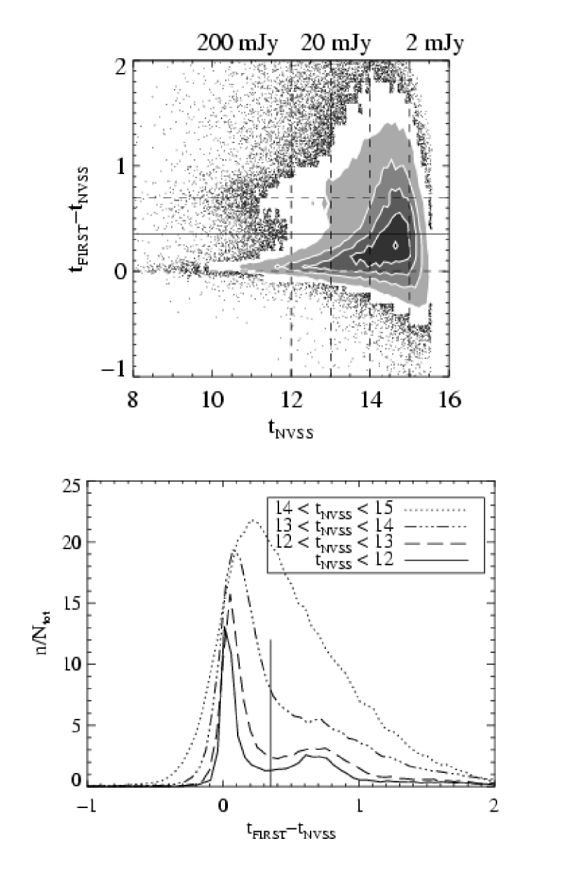
Figure 6: Top: Difference in 20 cm radio magnitudes measured by FIRST and NVSS as a function of $t_{\mathrm{NVSS}}$. Where individual points saturate the plot, we show the distribution using contours. The dashed horizontal lines indicate peaks at $\Delta t=0$ and $\Delta t=0.7$. The solid horizontal line shows the $\Delta t=0.35$ separator between between complex and simple sources. Vertical dashed lines mark the magnitude bins shown in the lower panel. Bottom: Distribution in $\Delta t$ for four $t_{\mathrm{NVSS}}$ bins. The vertical solid line shows the $\Delta t=0.35$ separator between complex and simple sources.

Figure 11: The magnitude distribution of compact morphology radio sources, observed by all four radio surveys and brighter than $t_{\mathrm{NVSS}}=12$, categorized into four subclasses by spectral shape. Top: Representations of a standard spectral shape in each class, defined by radio fluxes at 6, 20, and 92 cm. Steep and flat refer to sources with monotonic radio flux measurements. Steep sources have $\alpha^{92}_{6}<-0.5$; flat sources have $\alpha^{92}_{6}>-0.5$. Peaked refers to sources which are brightest at 20 cm. Inverted refers to sources which are faintest at 20 cm. Middle: Twenty centimeter magnitude distribution for each spectral shape subclass. Bottom: Fraction of sources brighter than $t_{\mathrm{max}}$ belonging to each spectral shape class.

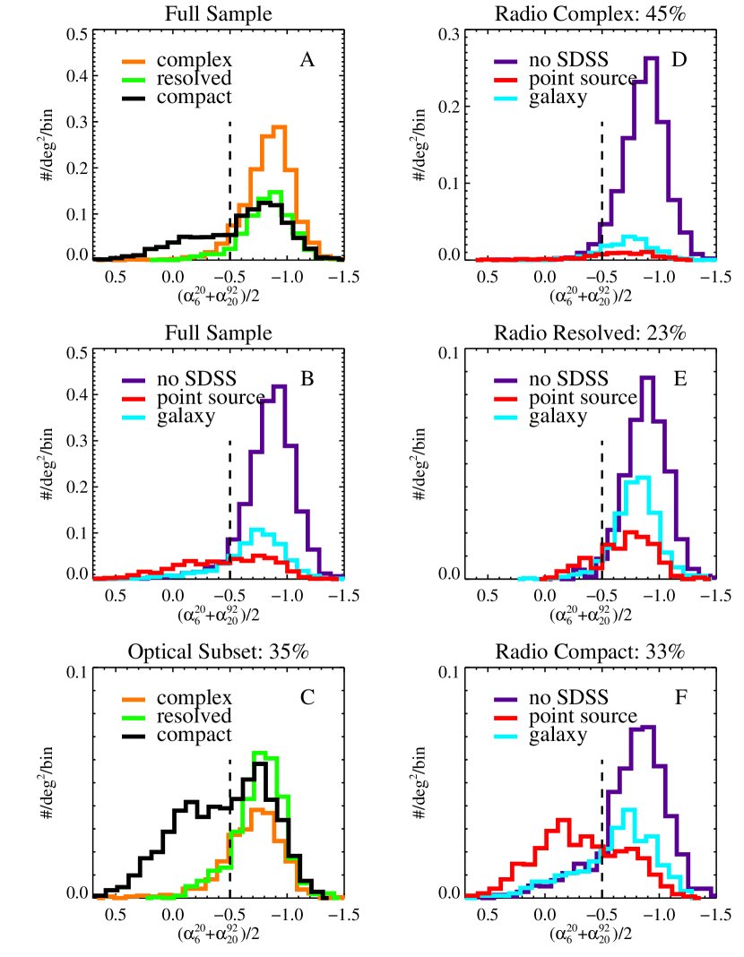
Figure 14: Distribution of the average of spectral indices $\alpha^{20}_{6}$ and $\alpha^{92}_{20}$ for $t_{\mathrm{NVSS}}<12$ sources detected in all four radio surveys. The vertical dashed lines show the separation between steep- and flat-spectrum sources. Note that the Y-axis range varies. Panel A: Full sample divided by radio morphology. Panel B: Full sample divided by optical identification. Panel C: Optically-identified sources divided by radio morphology. Panels D-F: Complex, resolved, and compact radio sources, respectively.

Figure 18: A simulated radio spectrum for which $\alpha^{92}_{20}$ would appear flat at high redshift (z) and steep at low redshift. Observed 20 and 92 cm fluxes correspond to shorter rest-frame wavelengths for a high-redshift object.

Figure 22: Examples of different types of sources found by matching NVSS and FIRST. Circles represent NVSS detections; squares represent FIRST detections. The sizes of the two types of symbols help illustrate the different spatial resolution of the two surveys. Quadrant A contains a complex source resolved into three components by FIRST but unresolved by NVSS, as well as a fourth (unrelated) FIRST detection. Quadrant B contains a simple source identified by both surveys, with no nearby neighbors. Quadrant C contains a FIRST detection with no NVSS counterpart, while Quadrant D contains a NVSS detection with no FIRST counterpart.

Table 1: Technical comparison of the radio source surveys.

statistics	FIRST	NVSS	GB6	WENSS
Frequency [MHz]	1400	1400	5000	326
Wavelength [cm]	20	20	6	92
Resolution [arcsec]	5	45	210	54
Sky coverage	$b>30\arcdeg$	$\delta>-40\arcdeg$	$0<\delta<75$	$\delta>30\arcdeg$
Sky area [$\deg^{-2}$]	10,000	33,000	17,000	10,000
Lim. Flux density	1	2.5	18	18
($5\sigma_{rms}$, mJy)
Lim. AB mag	16.4	15.4	13.3	13.3
Source density [$\deg^{-2}$]	97	55	4.4	22

Table 2: Completeness and efficiency as a function of matching radius

Matched surveys	Radius [arcsec]	Completeness	Efficiency
FIRST-NVSS	25	0.990	0.96
	30	0.997	0.96
FIRST-WENSS	30	0.990	0.92
	120	1.000	0.74
FIRST-GB6	70	0.979	0.79
	120	1.000	0.68
FIRST-SDSS	2	0.982	0.95
	3	0.998	0.90
	10	1.000	0.47
NVSS-WENSS	55	0.910	0.85
	120	0.995	0.57

Note. — To calculate these values, the nearest neighbor distributions were fit to a Gaussian (representing physical matches) plus a rising linear function (representing random matches).

Table 3: Double-Gaussian fits to FIRST-NVSS $\Delta t$ distributions

Bin	Simple sources			Complex sources
	Fraction	Mean	$\sigma$	Fraction	Mean	$\sigma$
$t_{\mathrm{NVSS}}<12$	0.59	0.035	0.044	0.41	0.58	0.35
$12<t_{\mathrm{NVSS}}<13$	0.67	0.064	0.074	0.33	0.64	0.37
$13<t_{\mathrm{NVSS}}<14$	0.65	0.12	0.13	0.35	0.75	0.47
$14<t_{\mathrm{NVSS}}<15$	0.59	0.23	0.24	0.41	0.75	0.49

Note. — The distributions are shown in the lower panel of Figure 6.

Table 4: Comparison of automatic and visual morphology classification

Visual	Total		Complex (%)		Resolved (%)		Compact (%)
Classification	QSOs	Gals.	QSOs	Gals.	QSOs	Gals.	QSOs	Gals.
Complex	202	286	77	95	8	4	15	1
Resolved	87	79	8	42	72	58	20	0
Compact	273	144	5	26	9	26	86	48

Note. — Results compiled for a set of 1071 radio quasars and radio galaxies (identified spectroscopically from the SDSS). Visual classification is listed at the left; automatic classification is listed along the top.

Table 5: Gaussian fits to $(\alpha^{92}_{20}+\alpha^{20}_{6})/2$ distributions

Subclass	$\deg^{-2}$	mean	median	FWHM
Complex
All	1.3	-0.868	-0.863	0.433
no SDSS	1.1	-0.886	-0.881	0.406
galaxy	0.15	-0.742	-0.732	0.433
pt. source	0.069	-0.705	-0.662	0.629
Resolved
All	0.68	-0.850	-0.843	0.433
no SDSS	0.38	-0.895	-0.892	0.416
galaxy	0.19	-0.808	-0.805	0.385
pt. source	0.11	-0.742	-0.733	0.571
Compact
All	0.99	-0.713	-0.680	0.822
no SDSS	0.45	-0.839	-0.815	0.530
galaxy	0.24	-0.710	-0.670	0.682
pt. source	0.30	-0.302	-0.288	1.03

Note. — Values correspond to histograms shown in Figure 14. Sources were detected by all four radio surveys, and follow the additional constraint $t_{\mathrm{NVSS}}<12$.

Table 6: Gaussian fits to $\alpha^{92}_{20}$ distributions

Subclass	$\deg^{-2}$	mean	median	FWHM
Complex
All	1.3	-0.786	-0.782	0.323
no SDSS	1.1	-0.798	-0.797	0.301
galaxy	0.15	-0.659	-0.654	0.323
pt. source	0.069	-0.718	-0.690	0.396
Resolved
All	0.68	-0.764	-0.765	0.339
no SDSS	0.38	-0.807	-0.817	0.320
galaxy	0.19	-0.700	-0.702	0.311
pt. source	0.11	-0.713	-0.710	0.378
Compact
All	0.99	-0.632	-0.563	0.640
no SDSS	0.45	-0.727	-0.683	0.440
galaxy	0.24	-0.593	-0.553	0.576
pt. source	0.30	-0.271	-0.229	1.05

Note. — Values correspond to the data samples investigated in Fig. 14 and Table 5. Sources were detected by all four radio surveys, and follow the additional constraint $t_{\mathrm{NVSS}}<12$. The $\alpha^{92}_{20}$ histograms are not shown.

Table 7: Candidate radio star selection

Data Source	All	in FIRST	$i<19.0$	Non-QSO colors	w/ spec.	stellar spec.
opt. point sources	19,133,672	12,100	2,424	532	406	78
quasar catalog	35,450	2,927	1,761	289	289	2
	(37,010)	(3,147)	(1,931)	(358)	(358)	(2)

Note. —

Table 8: Catalog subsets available for download

Sample	Description	Selection	# rows	size
A	Complete catalog	None	2,724,343	257M (1.4G)
B	$100\deg^{2}$ subset	$140\arcdeg<$ra$<165\arcdeg$	16,453	3.4M (15M)
		$40\arcdeg<$dec$<50\arcdeg$
C	Detected by FIRST	overlap = 1	141,881	5.4M (8.7M)
	and NVSS	matchflag_nvss $=-1$
		matchflag_first = 1
		distance $\leq 25\arcsec$
D	Detected by FIRST,	(subset of C)	63,660	-
	NVSS, and WENSS	wenss_flux $\neq 0$
		wenss_distance $\leq 30\arcsec$
E	Detected by FIRST,	(subset of D)	12,414	-
	NVSS, WENSS,	gb6_flux $\neq 0$
	and GB6	gb6_distance $\leq 70\arcsec$
F	Detected by FIRST,	(subset of E)	4,732	625K
	NVSS, WENSS, GB6,	near_type $\neq 0$
	and SDSS	near_distance $\leq 2\arcsec$
G	Spectroscopic galaxies	(subset of D)	2,885	439K
	detected by FIRST,	spec_type $=2$
	NVSS, WENSS,	near_distance $\leq 2\arcsec$
	and SDSS
H	Spectroscopic quasars	(subset of C)	1,288	755K
	detected by FIRST,	Match to Schneider et
	NVSS, WENSS, SDSS	al. (2007) within $2\arcsec$
I	Isolated FIRST-NVSS	(subset of C)	109,825	4.1M (6.8M)
		distance $\leq 15\arcsec$
		No other FIRST
		sources within $30\arcsec$
J	Isolated FIRST-NVSS,	(subset of I)	44,851	3.7M (5.7M)
	and SDSS	near_type $\neq 0$
		near_distance $\leq 2\arcsec$
K	Candidate high-	(subset of E)	9,619	2.5M (5.1M)
	redshift galaxies	(near_ra=0 OR
	($z\gtrsim 1$)	near_distance $>3\arcsec$)
		$\alpha^{92}_{20}\leq-0.5,\,\alpha^{20}_{6}\leq-0.5$
		remove suspicious
		objects (§5.2)

Note. — The first column gives the subset identifier, the second column contains a brief description, the third column lists the requirements to select the data set from the complete catalog, and the fourth column shows the number of sources in the data set. The fifth column indicates the size of the downloadable file for datasets available (with limited data parameters) on the catalog website. For compressed files, the uncompressed size is listed in parentheses.

References

- Adelman-McCarthy et al. (2007) Adelman-McCarthy, J. K. et al. 2007, ApJS, 172, 634
- Antonucci (1993) Antonucci, R. 1993, ARA&A, 31, 473
- Barai & Wiita (2006) Barai, P., & Wiita, P. J. 2006, MNRAS, 372, 381
- Barai & Wiita (2007) —. 2007, ApJ, 658, 217
- Barthel (1989) Barthel, P. D. 1989, ApJ, 336, 606
- Barvainis et al. (2005) Barvainis, R., Lehár, J., Birkinshaw, M., Falcke, H., & Blundell, K. M. 2005, ApJ, 618, 108
- Becker et al. (1995) Becker, R. H., White, R. L., & Helfand, D. J. 1995, ApJ, 450, 559
- Best et al. (2005) Best, P. N., Kauffmann, G., Heckman, T. M., & Ivezić, Ž. 2005, MNRAS, 362, 9
- Blundell & Rawlings (2000) Blundell, K. M., & Rawlings, S. 2000, AJ, 119, 1111
- Blundell et al. (1999) Blundell, K. M., Rawlings, S., & Willott, C. J. 1999, AJ, 117, 677
- Chanmugam (1987) Chanmugam, G. 1987, Ap&SS, 130, 53
- Colless et al. (2001) Colless, M. et al. 2001, MNRAS, 328, 1039
- Condon (1984) Condon, J. J. 1984, ApJ, 287, 461
- Condon et al. (1998) Condon, J. J., Cotton, W. D., Greisen, E. W., Yin, Q. F., Perley, R. A., Taylor, G. B., & Broderick, J. J. 1998, AJ, 115, 1693
- Cruz et al. (2006) Cruz, M. J. et al. 2006, MNRAS, 373, 1531
- De Breuck (2000) De Breuck, C. 2000, PhD thesis
- de Vries et al. (2007) de Vries, N., Snellen, I. A. G., Schilizzi, R. T., Lehnert, M. D., & Bremer, M. N. 2007, A&A, 464, 879
- de Vries et al. (2006) de Vries, W. H., Becker, R. H., & White, R. L. 2006, AJ, 131, 666
- de Vries et al. (2004) de Vries, W. H., Becker, R. H., White, R. L., & Helfand, D. J. 2004, AJ, 127, 2565
- de Vries et al. (2002) de Vries, W. H., Morganti, R., Röttgering, H. J. A., Vermeulen, R., van Breugel, W., Rengelink, R., & Jarvis, M. J. 2002, AJ, 123, 1784
- Eales (1985) Eales, S. A. 1985, MNRAS, 217, 149
- Eisenstein et al. (2001) Eisenstein, D. J. et al. 2001, AJ, 122, 2267
- Fanaroff & Riley (1974) Fanaroff, B. L., & Riley, J. M. 1974, MNRAS, 167, 31P
- Fukugita et al. (1996) Fukugita, M., Ichikawa, T., Gunn, J. E., Doi, M., Shimasaku, K., & Schneider, D. P. 1996, AJ, 111, 1748
- Gregory et al. (1996) Gregory, P. C., Scott, W. K., Douglas, K., & Condon, J. J. 1996, ApJS, 103, 427
- Gregory et al. (1994) Gregory, P. C., Vavasour, J. D., Scott, W. K., & Condon, J. J. 1994, ApJS, 90, 173
- Gunn et al. (1998) Gunn, J. E. et al. 1998, AJ, 116, 3040
- Hughes et al. (1989) Hughes, P. A., Aller, H. D., & Aller, M. F. 1989, ApJ, 341, 68
- Ivezić et al. (2003) Ivezić, Ž. et al. 2003, Memorie della Societa Astronomica Italiana, 74, 978
- Ivezić et al. (2004a) —. 2004a, Astronomische Nachrichten, 325, 583
- Ivezić et al. (2002) —. 2002, AJ, 124, 2364
- Ivezić et al. (2004b) Ivezić, Ž. et al. 2004b, in Astronomical Society of the Pacific Conference Series, Vol. 311, AGN Physics with the Sloan Digital Sky Survey, ed. G. T. Richards & P. B. Hall, 347
- Jackson & Wall (1999) Jackson, C. A., & Wall, J. V. 1999, MNRAS, 304, 160
- Jarvis & McLure (2006) Jarvis, M. J., & McLure, R. J. 2006, MNRAS, 369, 182
- Jones et al. (2004) Jones, D. H. et al. 2004, MNRAS, 355, 747
- Kellermann (1964) Kellermann, K. I. 1964, ApJ, 140, 969
- Krolik (1999) Krolik, J. H. 1999, Active galactic nuclei : from the central black hole to the galactic environment (Princeton, N. J. : Princeton University Press, c1999.)
- Kuehr et al. (1981) Kuehr, H., Witzel, A., Pauliny-Toth, I. I. K., & Nauber, U. 1981, A&AS, 45, 367
- Laing et al. (1983) Laing, R. A., Riley, J. M., & Longair, M. S. 1983, MNRAS, 204, 151
- Lister et al. (1994) Lister, M. L., Hutchings, J. B., & Gower, A. C. 1994, ApJ, 427, 125
- Lu et al. (2007) Lu, Y., Wang, T., Zhou, H., & Wu, J. 2007, AJ, 133, 1615
- Lupton et al. (2002) Lupton, R. H., Ivezic, Z., Gunn, J. E., Knapp, G., Strauss, M. A., & Yasuda, N. 2002, in Proc. SPIE, 4836, 350
- Machalski & Condon (1999) Machalski, J., & Condon, J. J. 1999, ApJS, 123, 41
- Madau et al. (1996) Madau, P., Ferguson, H. C., Dickinson, M. E., Giavalisco, M., Steidel, C. C., & Fruchter, A. 1996, MNRAS, 283, 1388
- Magliocchetti et al. (2002) Magliocchetti, M. et al. 2002, MNRAS, 333, 100
- Marscher & Gear (1985) Marscher, A. P., & Gear, W. K. 1985, ApJ, 298, 114
- Mason & Gray (2007) Mason, P. A., & Gray, C. L. 2007, ApJ, 660, 662
- Massardi et al. (2008) Massardi, M. et al. 2008, MNRAS, 384, 775
- Mauch et al. (2003) Mauch, T., Murphy, T., Buttery, H. J., Curran, J., Hunstead, R. W., Piestrzynski, B., Robertson, J. G., & Sadler, E. M. 2003, MNRAS, 342, 1117
- Mauch & Sadler (2007) Mauch, T., & Sadler, E. M. 2007, MNRAS, 375, 931
- McGilchrist et al. (1990) McGilchrist, M. M., Baldwin, J. E., Riley, J. M., Titterington, D. J., Waldram, E. M., & Warner, P. J. 1990, MNRAS, 246, 110
- Napier (2006) Napier, P. J. 2006, in Astronomical Society of the Pacific Conference Series, Vol. 356, Revealing the Molecular Universe: One Antenna is Never Enough, ed. D. C. Backer, J. M. Moran, & J. L. Turner, 65
- O’Dea (1998) O’Dea, C. P. 1998, PASP, 110, 493
- Oke & Gunn (1983) Oke, J. B., & Gunn, J. E. 1983, ApJ, 266, 713
- Padmanabhan et al. (2005) Padmanabhan, N. et al. 2005, MNRAS, 359, 237
- Padovani & Urry (1992) Padovani, P., & Urry, C. M. 1992, ApJ, 387, 449
- Pier et al. (2003) Pier, J. R., Munn, J. A., Hindsley, R. B., Hennessy, G. S., Kent, S. M., Lupton, R. H., & Ivezić, Ž. 2003, AJ, 125, 1559
- Rengelink et al. (1997) Rengelink, R. B., Tang, Y., de Bruyn, A. G., Miley, G. K., Bremer, M. N., Roettgering, H. J. A., & Bremer, M. A. R. 1997, A&AS, 124, 259
- Richards et al. (2002) Richards, G. T. et al. 2002, AJ, 123, 2945
- Richards et al. (2001) —. 2001, AJ, 121, 2308
- Rys & Machalski (1990) Rys, S., & Machalski, J. 1990, A&A, 236, 15
- Sadler et al. (2002) Sadler, E. M. et al. 2002, MNRAS, 329, 227
- Sadler et al. (1999) Sadler, E. M., McIntyre, V. J., Jackson, C. A., & Cannon, R. D. 1999, Publications of the Astronomical Society of Australia, 16, 247
- Schlegel et al. (1998) Schlegel, D. J., Finkbeiner, D. P., & Davis, M. 1998, ApJ, 500, 525
- Schneider et al. (2007) Schneider, D. P. et al. 2007, AJ, 134, 102
- Scranton et al. (2002) Scranton, R. et al. 2002, ApJ, 579, 48
- Stoughton et al. (2002) Stoughton, C. et al. 2002, AJ, 123, 485
- Strauss et al. (2002) Strauss, M. A. et al. 2002, AJ, 124, 1810
- Urry & Padovani (1995) Urry, C. M., & Padovani, P. 1995, PASP, 107, 803
- Urry et al. (1991) Urry, C. M., Padovani, P., & Stickel, M. 1991, ApJ, 382, 501
- Vanden Berk et al. (2005) Vanden Berk, D. E. et al. 2005, AJ, 129, 2047
- White et al. (1989) White, S. M., Jackson, P. D., & Kundu, M. R. 1989, ApJS, 71, 895
- Willott et al. (2002) Willott, C. J., Rawlings, S., Archibald, E. N., & Dunlop, J. S. 2002, MNRAS, 331, 435
- York et al. (2000) York, D. G. et al. 2000, AJ, 120, 1579
- Zhang et al. (2003) Zhang, X., Reich, W., Reich, P., & Wielebinski, R. 2003, A&A, 404, 57