Symmetry of superconducting states with two orbitals on a tetragonal lattice: application to $LaFeAsO_{1-x}F_{x}$

Abstract

We use group theory to classify the superconducting states of systems with two orbitals on a tetragonal lattice. The orbital part of the superconducting gap function can be either symmetric or anti-symmetric. For the orbital symmetric state, the parity is even for spin singlet and odd for spin triplet; for the orbital anti-symmetric state, the parity is odd for spin singlet and even for spin triplet. The gap basis functions are obtained with the use of the group chain scheme by taking into account the spin-orbit coupling. In the weak pairing limit, the orbital anti-symmetric state is only stable for the degenerate orbitals. Possible application to iron-based superconductivity is discussed.

I Introduction

Symmetry plays an important role in the study of superconductivity. By using the symmetry of the superconducting (SC) gap function, Ginzburg-Landau theory can be constructed and electromagnetic response and topological excitations can be inspected. In the past decades, the symmetry analyses to classify unconventional SC states have been focused on single-band superconductors, and have shed much light on our understanding of heavy-fermion and ruthenate superconductorsSigrist91 .

Very recently, a new class of iron-based high temperature superconductors has been discovered with $T_{c}$ as high as above $50$KLOFS ; COFS ; SOFS ; POFS ; SOFS2 ; GOFS ; SOxFS2 ; Hole . Experimentally, spin density wave (SDW) order has been observed in the parent compound $LaFeAsO$, but vanishes upon fluorine doping where the superconductivity appearsSDW ; Neutron . Specific heat measurement as well as nuclear magnetic resonance suggested line nodes of the SC gapCV ; NMR ; NMR2 ; NMR3 . The transition temperature estimated based on the electron-phonon coupling is low, and unlikely to explain the observed superconductivityBoeri . It has been proposed that the superconductivity is of magnetic origin and is unconventional. Local density approximation (LDA) shows that iron’s $3d$ electrons dominate the density of states near the Fermi surfaces in the parent compound $LaFeAsO$LDA1Singh ; LDA2Kotliar ; LDA3Xu ; LDA4Mazin ; LDA5Cao ; LDA6Ma . In their calculations, there are three hole-like Fermi surfaces centered at the $\Gamma$ point and two electron-like Fermi surfaces around the $M$ point. By F-doping, the area of the three hole-like Fermi surfaces shrinks while the area of the two electron-like Fermi surfaces expands. The band structure obtained from the LDA may be well modeled by a tight-binding model with two or three orbitals ($d_{xz}$, $d_{yz}$ and $d_{xy})$ Theory1Dai ; Theory2LiTao ; Theory3Xiaogang ; Theory4ZYWeng ; Theory5Shoucheng ; Theory6Zidan ; Theory7Qimiao ; Theory8Scalapino . Because of the multiple orbitals in the low energy physics, it is natural to raise the question how to generalize the symmetry consideration from single-band to multi-band cases.

In this paper, we will generalize the symmetry analyses developed for the single band SC state to systems with two orbitals. We will use group theory to classify the allowed symmetry of the gap functions of the two-orbital SC state on a tetragonal lattice by including a spin-orbit coupling between the paired electrons. While our focus will be on the Fe-based compounds, some of our analyses may be applied to more general systems with two orbitals.

We arrange this paper as the follows. In Sec. II, we discuss the symmetries governing the system and how these symmetries affect the Hamiltonian and gap functions. In Sec. III, we consider the possible two-orbital SC states on a tetragonal lattice. Section IV is devoted to summary and discussions. We also supply some appendixes for details. In Appendix A, we show how the symmetries give rise to the requirements to the non-interacting Hamiltonian. In Appendix B, we specify the point group $D_{4h}$ of lattice according to space group $P4/nmm$. In Appendix C, we discuss how the gap functions transfer under symmetry operations. In Appendix D, we discuss the energy gap functions in the degenerate bands.

II Symmetry of gap function $\Delta\left(\mathbf{k}\right)$

We consider a tetragonal lattice, appropriate for doped $LaFeAsO$. Since our primary interest is in the SC state, we will not consider the translational symmetry broken state such as the spin density wave state observed in the parent compound of $LaFeAsO$. The system is invariant under both time reversal and space inversion. The inversion symmetry suggests that the SC pairing is either even or odd in parity. We shall assume in this paper that the time reversal symmetry remains unbroken.

We consider a system described by Hamiltonian

$$H=H_{0}+H_{pair}+H_{so}$$ (1)

where $H_{0}$ is non-interacting part, and $H_{pair}$ is a pairing Hamiltonian, and $H_{so}$ is the spin-orbit coupling of the Cooper pairs. We shall consider the SC state preserves all the symmetries in $H_{0}$ except the $U(1)$ symmetry in electric charge and the spin rotational symmetry due to a weak $H_{so}$. We assume $H_{0}$ to be given by a tight-binding Hamiltonian

$$H_{0}=\sum\limits_{\mathbf{k}\alpha_{1}\alpha_{2}s}c_{\mathbf{k}\alpha_{1}s}^{\dagger}\xi_{\mathbf{k\alpha}_{1}\alpha_{2}}c_{\mathbf{k}\alpha_{2}s},$$ (2)

where $\alpha=1,2$ are the orbital indices, which correspond to the two orbitals $3d_{xz}$ and $3d_{yz}$ in $Fe$, $s=\uparrow,\downarrow$ are the spin indices. Note that for $LaFeAsO$, the actual crystal structure has two Fe-atoms in a unit cell due to the $As$ atomic positions, which are allocated above and below the Fe-plane alternatively. For convenience, here we use the extended Brillouine zone, and the summation $\mathbf{k}$ is in the extended zone. $H_{0}$ is invariant under symmetry transformation. This requires certain symmetries on $\xi_{\mathbf{k\alpha}_{1}\alpha_{2}}$, which we will discuss in detail in Appendix A. We note that a more appropriate model should also include the $d_{xy}$-orbitalTheory3Xiaogang , but we shall leave the symmetry analyses of the three orbitals for future study, and consider a simplified version of the two orbital case in this paper.

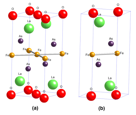
Figure 1: (color online) Lattice structure of $LaFeAsO$. It is a tetragonal lattice with two $Fe$ atoms per unit cell. The lattice constants are $a=b\simeq 4.03\mathring{A}$ and $c\simeq 8.74\mathring{A}$Neutron , where $a$ is the distance between two next nearest neighbor $Fe$ atoms. (a) Origin choice 1 of space group $P4/nmm$, at $\bar{4}m2$ and at $(-a/4,a/4,0)$ from center ($2/m$). It can be chosen either at an $Fe$ or at an $O$ atom; (b) Origin choice 2 of space group $P4/nmm$, at center ($2/m$) and at $(a/4,-a/4,0)$ from $\bar{4}m2$. It can be chosen either at the midpoint of two nearest neighbor $Fe$ atoms or at the midpoint of two nearest neighbor $O$ atoms. Here $2/m$ denotes the two fold rotation $C_{2}$ and reflection $m$ (see Appendix B for details). The origin choice 1 and 2 are different from each other by a shift of $(-a/4,a/4,0)$crystallography .

The gap function of the two-orbital SC state can be generally written as

$$\Delta_{s_{1}s_{2}}^{\alpha_{1}\alpha_{2}}\left(\mathbf{k}\right)=-\sum\limits_{\begin{subarray}{c}\mathbf{k}^{\prime}\alpha_{3}\alpha_{4}\\ s_{3}s_{4}\end{subarray}}V_{s_{2}s_{1}s_{3}s_{4}}^{\alpha_{2}\alpha_{1}\alpha_{3}\alpha_{4}}\left(\mathbf{k},\mathbf{k}^{\prime}\right)\langle c_{\mathbf{k}^{\prime}\alpha_{3}s_{3}}c_{-\mathbf{k}^{\prime}\alpha_{4}s_{4}}\rangle,$$ (3)

where $V_{s_{2}s_{1}s_{3}s_{4}}^{\alpha_{2}\alpha_{1}\alpha_{3}\alpha_{4}}\left(\mathbf{k},\mathbf{k}^{\prime}\right)$ is the effective attractive interaction. Hereafter we will use the matrix notation $\Delta\left(\mathbf{k}\right)$ for the gap function.

To classify the symmetry of the SC gap function for multiple orbitals, we recall that in the single orbital case, the spin-orbit coupling of the Cooper pair plays an important role to the non s-wave superconductors, and the symmetry of the gap function is determined by the crystal point group of the lattice and the spin part of the gap function. In the two-orbital system, the orbital degree of freedom is usually coupled to the crystal momentum, hence to the spin via the spin-orbit coupling. Therefore, the spin, spatial, and the orbital parts are generally all related in the gap function.

Let us first discuss the crystal symmetry. The crystal structure of $LaFeAsO$ is shown in Fig. 1. The tetragonal crystal symmetry is characterized by the point group $D_{4h}$. The tetragonal point group may be specified according to the space group $P4/nmm$ of the compound, and the details will be discussed in Appendix B. There are five irreducible representations of $D_{4}$ group, denoted by $\Gamma$, including 4 one-dimensional representations ($A_{1}$, $A_{2}$, $B_{1}$ and $B_{2}$) and 1 two-dimensional representation ($E$)Butler . The tetragonal lattice symmetry requires $H_{0}$ to be a “scalar” or $A_{1}$ representation of $D_{4}$. In the absence of spin-orbit coupling, spin is rotational invariant and we have both the point group symmetry and the spin rotational symmetry.P4nmm

We now discuss the orbital degrees of freedom in connection with the crystal symmetry. The two orbitals $d_{xz}$ and $d_{yz}$ transform as $E$ representation of $D_{4}$. In general the orbital indices $d_{xz}$ and $d_{yz}$ are not good quantum numbers because of the mixed term of the two orbitals in $H_{0}$, and the two energy bands are not degenerate. In that case it is necessary to include the coupling of the orbital to spatial and spin degrees of freedom.

Without loss of generality, the gap function can be written as a linear combination of the direct products of the orbital part $\Omega$ and the spin part $\Delta^{spin}$ in a given representation $\Gamma$ of the point group $D_{4}$,

$$\Delta\left(\Gamma;\mathbf{k}\right) = \sum\limits_{m,\Gamma_{LS},\Gamma_{\Omega}}\eta\left(\Gamma,m\right)\left\langle\Gamma,m|\Gamma_{LS},m_{LS};\Gamma_{\Omega},m_{\Omega}\right\rangle$$ (4)

$$\times\Delta^{spin}\left(\Gamma_{LS},m_{LS};\mathbf{k}\right)\otimes\Omega\left(\Gamma_{\Omega},m_{\Omega}\right),$$

where both $\Delta^{spin}$ and $\Omega$ are $2\times 2$ matrices, $\Delta_{s_{1}s_{2}}^{spin}$ dictates the pairing in spin space and $\Omega_{\alpha_{1}\alpha_{2}}$ dictates the pairing in orbital space, $\Gamma_{LS}$ and $\Gamma_{\Omega}$ are irreducible representations of $D_{4}$ in spin and orbital spaces, respectively, $m,m_{LS},m_{\Omega}$ are bases of representations $\Gamma,\Gamma_{LS},\Gamma_{\Omega}$, respectively. $\left\langle\Gamma,m|\Gamma_{LS},m_{LS};\Gamma_{\Omega},m_{\Omega}\right\rangle$ is the Clebsch-Gordan (CG) coefficient. Note that the $\mathbf{k}$-dependence is contained in $\Delta^{spin}$, but not in $\Omega$. Here $\eta\left(\Gamma,m\right)$ is the coefficient of the basis $m$ of the representation $\Gamma$. The anti-symmetric statistics of two electrons requires

$$\Delta^{T}\left(-\mathbf{k}\right)=-\Delta\left(\mathbf{k}\right).$$ (5)

Below we will first discuss $\Delta^{spin}\left(\Gamma_{LS};\mathbf{k}\right)$ and $\Omega\left(\Gamma_{\Omega}\right)$ separately, and then combine the two to form an irreducible representation $\Gamma$ of $D_{4}$. We follow Sigrist and UedaSigrist91 and write $\Delta^{spin}\left(\mathbf{k}\right)$ in terms of the basis functions $\psi\left(\Gamma,m;\mathbf{k}\right)$ for the spin singlet $S=0$ and $\mathbf{d}\left(\Gamma,m;\mathbf{k}\right)$ for the spin triplet $S=1$,

$$\Delta^{spin}\left(\Gamma,m;\mathbf{k}\right)=i\left[\sigma_{0}\psi\left(\Gamma,m;\mathbf{k}\right)+\mathbf{\sigma}\cdot\mathbf{d}\left(\Gamma,m;\mathbf{k}\right)\right]\sigma_{2},$$ (6)

Here $\psi\left(\mathbf{k}\right)$ is a scalar and $\mathbf{d}\left(\mathbf{k}\right)$ is a vector under the transformation of spin rotation. For this reason, it is more convenient to use $\psi\left(\mathbf{k}\right)$ and $\mathbf{d}\left(\mathbf{k}\right)$ instead of $\Delta^{spin}\left(\mathbf{k}\right)$ to classify the pairing states.

Due to the fermionic anti-symmetric nature, the gap function must be anti-symmetric under the two particle interchange, or under a combined operations of space inversion, interchange of the spin indices and interchange of the orbital indices of the two particles. Let $P_{1,2}$ be the two particle interchange operator, and $P_{space},P_{spin},P_{orbital}$ be the interchange operator acting on the space, spin, and orbital, respectively, then the fermion statistics requires

$$P_{1,2}=P_{space}P_{spin}P_{orbital}=-1.$$ (7)

Since the system is of inversion symmetry, the pairing states must have either even parity $P_{space}=+1$ or odd parity $P_{space}=-1$. Furthermore, the total spin $S$ of the Cooper pair is a good number, and this is so even in the presence of $H_{so}$, which breaks spin rotational symmetry but keeps inversion symmetry, so that it does not mix the $S=1$ with $S=0$ states. Therefore, under the two particle interchange, the spin part of the gap function must be either symmetric: ($P_{spin}=+1$, with $S=1$) or anti-symmetric ($P_{spin}=-1$ with $S=0$), represented by the vector $\mathbf{d}$ or the scalar $\psi$ in Eq. (6), respectively. Because of the inversion and spin symmetries, we have $P_{orbital}=\pm 1$.

The orbital part of the pairing matrix $\Omega$ is spanned in the vector space of $\left(d_{xz},d_{yz}\right)$, which is an irreducible representation $E$ of the point group $D_{4}$. Thus $\Omega$ belongs to an irreducible representation given by $E\otimes E=A_{1}\oplus A_{2}\oplus B_{1}\oplus B_{2}$, which are all one-dimensional, hence simplifies the classification of the pairing states. According to the CG coefficients of $D_{4}$ group, up to a global factor, $\Omega=\sigma_{0}$ in representation $A_{1}$, $\Omega=\sigma_{3}$ in $B_{1}$, and $\Omega=\sigma_{1}$ in $B_{2}$, which are all orbital symmetric: $P_{orbital}=+1$. $\Omega=\sigma_{2}$ in $A_{2}$ representation, which is orbital anti-symmetric: $P_{orbital}=-1$. In brief, $A_{1}$ and $B_{1}$ of $\Omega$ are representations for intra-orbital pairing, $B_{2}$ is for symmetric inter-orbital pairing and $A_{2}$ is for anti-symmetric inter-orbital pairing. For convenience, we choose $\Omega$ to be Hermitian, so that $\psi\left(\mathbf{k}\right)$ and $\mathbf{d}\left(\mathbf{k}\right)$ will be real. (Wan and WangQHWang pointed out that Pauli matrices transfer as four one-dimensional irreducible representations.)

The crystal point group of the lattice will dictate the allowed symmetry in $\mathbf{k}$ space. The transformation of $\psi$ and $\mathbf{d}$ under symmetry operations can be found in Appendix C. In Sec. III, we will study the basis functions $\psi\left(\Gamma,m;\mathbf{k}\right)$ and $\mathbf{d}\left(\Gamma,m;\mathbf{k}\right)$, and combine them with the orbital part $\Omega$ to obtain the irreducible representations of group $D_{4}$.

III Possible two-orbital SC states on a tetragonal lattice

We will use the group chain scheme to study the representation and the basis function of $\psi$ and $\mathbf{d}$ by assuming a spin-orbit coupling. In the group chain scheme, we begin with a rotational invariant system in both spin and spatial spaces. The representation of its symmetry group $G$ can be decoupled into a spatial part $D_{\left(L\right)}$ and a spin part $D_{\left(S\right)}$, with $\mathbf{L}$ as the relative angular momentum of the Cooper pair,

$$D_{\left(G\right)}=D_{\left(L\right)}\otimes D_{\left(S\right)},$$ (8)

In the presence of the spin-orbit coupling, $D_{\left(L\right)}$ and $D_{\left(S\right)}$ are no longer the irreducible representation of the rotational group, but the total angular momentum $\mathbf{J}=\mathbf{L}+\mathbf{S}$ is, and $D_{\left(J\right)}$ is the corresponding irreducible representation of the rotational group.

We now turn on a crystal field with tetragonal lattice symmetry group $D_{4}$, so that the rotational group $SO(3)$ is reduced to $D_{4}$, and $D_{\left(L\right)}\otimes D_{\left(S\right)}$ is reduced to a direct product of irreducible representations $\Gamma_{LS}$ of group $D_{4}$,

$$D_{\left(L\right)}\otimes D_{\left(S\right)}\rightarrow\bigoplus\limits_{\Gamma_{LS}}D_{\left(\Gamma_{LS}\right)}.$$ (9)

Including the coupling to the orbital part $\Omega$, the representation $D_{\left(\Gamma_{LS}\right)}\otimes D_{\left(\Gamma_{\Omega}\right)}$ is decomposed into irreducible representations,

$$D_{\left(\Gamma_{LS}\right)}\otimes D_{\left(\Gamma_{\Omega}\right)}=\bigoplus\limits_{\Gamma}D_{\left(\Gamma\right)}.$$ (10)

$D_{\left(\Gamma_{\Omega}\right)}$ is one-dimensional, thus these representations have a very simple form.

Let us consider the even parity case. From Eq. (7), the SC gap function can be either orbital symmetric $P_{orbital}=+1$, spin singlet or orbital anti-symmetric $P_{orbital}=-1$, spin triplet. We list the SC gap basis functions for spin singlet and spin triplet according to the irreducible representations $\Gamma$ in Tables I and II respectively. The listed even pairing states include $s$-wave (extended $s$-wave), $d$-wave and $g$-wave. Here $0$, $\tilde{0}$, $2$, $\tilde{2}$, and $1$ are natural notation for the five irreducible representations of $D_{4h}$; $A_{1}$, $A_{2}$, $B_{1}$, $B_{2}$ and $E$ are Schönflies notation; $\Gamma_{1-5}$ are Koster notation. According to Eq. (3), the gap function of the SC state is a linear combination of the basis functions in one irreducible representation $\Gamma$, and the basis functions belonging to different representations in $\Gamma$, e.g. $A_{1g}$ and $B_{2g}$, will not mix with each other.

We are particularly interested in 2D or quasi-2D limiting cases, relevant to Fe-based SC compounds, where the gap function is $k_{z}$-independent, and the Fermi surface is cylinder-like. However, for completeness we also list in the Tables those three-dimensional basic functions marked with 3D.

In the last column of each table, we list the allowed energy zeroes in the quasiparticle dispersion determined by the gap functions for the special case that the two energy bands are completely degenerate. The detailed calculations for the quasiparticle energies in the degenerate cases are given in Appendix D. We will discuss the quasiparticle properties for the non-degenerate cases in the discussion section below.

Table 1: Superconducting gap basis functions $\psi(\mathbf{k})$ on tetragonal lattice for even parity, orbital symmetric and spin singlet pairing states. $\Gamma$: representation of $D_{4}$. The listed notations are natural, or Schönflies and Koster (in parentheses). $\Omega$: orbital representation, $\sigma_{0}$ is the identity matrix, and $\sigma_{1,2,3}$ are Pauli matrices. Listed gaps properties are for the two completely degenerate orbitals. $k_{z}$-dependent basis functions are marked with $(3D)$, listed for completeness.

$\Gamma$	basis $\psi(\mathbf{k})$	$\Omega$	gap
	$1,k_{x}^{2}+k_{y}^{2};k_{z}^{2}$ (3D)	$\sigma_{0}$
$0$ ($A_{1g}$, $\Gamma_{1}^{+}$)	$k_{x}^{2}-k_{y}^{2}$	$\sigma_{3}$	line nodal, or full gap
	$k_{x}k_{y}$	$\sigma_{1}$
	$k_{x}k_{y}(k_{x}^{2}-k_{y}^{2})$	$\sigma_{0}$
$\tilde{0}$ ($A_{2g}$, $\Gamma_{2}^{+}$)	$k_{x}k_{y}$	$\sigma_{3}$	line,full
	$k_{x}^{2}-k_{y}^{2}$	$\sigma_{1}$
	$k_{x}^{2}-k_{y}^{2}$	$\sigma_{0}$
$2$ ($B_{1g}$, $\Gamma_{3}^{+}$)	$1,k_{x}^{2}+k_{y}^{2};k_{z}^{2}$ (3D)	$\sigma_{3}$	line,full
	$k_{x}k_{y}(k_{x}^{2}-k_{y}^{2})$	$\sigma_{1}$
	$k_{x}k_{y}$	$\sigma_{0}$
$\tilde{2}$ ($B_{2g}$, $\Gamma_{4}^{+}$)	$k_{x}k_{y}(k_{x}^{2}-k_{y}^{2})$	$\sigma_{3}$	line,full
	$1,k_{x}^{2}+k_{y}^{2};k_{z}^{2}$ (3D)	$\sigma_{1}$
$1$ ($E_{g}$, $\Gamma_{5}^{+}$)	$(k_{x}k_{z},k_{y}k_{z})$ (3D)	$\sigma_{0},\sigma_{3},\sigma_{1}$

Table 2: Superconducting gap basis functions $\mathbf{d}(\mathbf{k})$ on tetragonal lattice for even parity, orbital anti-symmetric and spin triplet pairing states. Notations are the same as in Table I.

$\Gamma$	basis $\mathbf{d}(\mathbf{k})$	$\Omega$	gap
$0$ ($A_{1g}$, $\Gamma_{1}^{+}$)	$\hat{z},(k_{x}^{2}+k_{y}^{2})\hat{z},(k_{x}^{4}+k_{y}^{4})\hat{z},k_{x}^{2}k_{y}^{2}\hat{z}$	$\sigma_{2}$	line,full
$\tilde{0}$ ($A_{2g}$, $\Gamma_{2}^{+}$)	$k_{z}(k_{x}\hat{y}-k_{y}\hat{x})$ (3D)	$\sigma_{2}$
$2$ ($B_{1g}$, $\Gamma_{3}^{+}$)	$(k_{x}^{2}-k_{y}^{2})\hat{z};k_{z}(k_{x}\hat{x}-k_{y}\hat{y})$ (3D)	$\sigma_{2}$	line
$\tilde{2}$ ($B_{2g}$, $\Gamma_{4}^{+}$)	$k_{x}k_{y}\hat{z};k_{z}(k_{x}\hat{x}+k_{y}\hat{y})$ (3D)	$\sigma_{2}$	line
$1$ ($E_{g}$, $\Gamma_{5}^{+}$)	$\begin{array}[]{c}(\hat{x},\hat{y}),(k_{x}^{2}\hat{x},k_{x}^{2}\hat{y}),(k_{y}^{2}\hat{x},k_{y}^{2}\hat{y}),(k_{x}k_{y}\hat{x},k_{x}k_{y}\hat{y});\\ (k_{z}^{2}\hat{x},k_{z}^{2}\hat{y}),(k_{x}k_{z}\hat{z},k_{y}k_{z}\hat{z})\text{ (3D)}\end{array}$	$\sigma_{2}$	line,full

Similarly, for the odd parity pairing $P_{space}=-1$, we can have either orbital anti-symmetric $P_{orbital}=-1$, spin singlet, or orbital symmetric $P_{orbital}=1$, spin triplet, which are listed in Tables III and IV respectively. For the spin triplet, we list $p$-wave, $f$-wave and $h$-wave states.

Table 3: Superconducting gap basis functions $\psi(\mathbf{k})$ on tetragonal lattice for odd parity, orbital anti-symmetric and spin singlet pairing state. Notations are the same as in Table I.

$\Gamma$	basis $\psi(\mathbf{k})$	$\Omega$	gap
$0$ ($A_{1u}$, $\Gamma_{1}^{-}$)	$k_{z}$ (3D)	$\sigma_{2}$
$\tilde{0}$ ($A_{2u}$, $\Gamma_{2}^{-}$)	$k_{z}(k_{x}^{4}-6k_{x}^{2}k_{y}^{2}+k_{y}^{4})$ (3D)	$\sigma_{2}$
$2$ ($B_{1u}$, $\Gamma_{3}^{-}$)	$k_{z}(k_{x}^{2}-k_{y}^{2})$ (3D)	$\sigma_{2}$
$\tilde{2}$ ($B_{2u}$, $\Gamma_{4}^{-}$)	$k_{x}k_{y}k_{z}$ (3D)	$\sigma_{2}$
$1$ ($E_{u}$, $\Gamma_{5}^{-}$)	$(k_{x},k_{y})$	$\sigma_{2}$	line

Table 4: Superconducting gap basis functions $\mathbf{d}(\mathbf{k})$ on tetragonal lattice for odd parity, orbital symmetric and spin triplet pairing states.

$\Gamma$	basis $\mathbf{d}(\mathbf{k})$	$\Omega$	gap
	$k_{x}\hat{x}+k_{y}\hat{y};k_{z}\hat{z}$ (3D)	$\sigma_{0}$
$0$ ($A_{1u}$, $\Gamma_{1}^{-}$)	$k_{x}\hat{x}-k_{y}\hat{y}$	$\sigma_{3}$	line,full
	$k_{y}\hat{x}+k_{x}\hat{y}$	$\sigma_{1}$
	$k_{y}\hat{x}-k_{x}\hat{y}$	$\sigma_{0}$
$\tilde{0}$ ($A_{2u}$, $\Gamma_{2}^{-}$)	$k_{y}\hat{x}+k_{x}\hat{y}$	$\sigma_{3}$	line,full
	$k_{x}\hat{x}-k_{y}\hat{y}$	$\sigma_{1}$
	$k_{x}\hat{x}-k_{y}\hat{y}$	$\sigma_{0}$
$2$ ($B_{1u}$, $\Gamma_{3}^{-}$)	$k_{x}\hat{x}+k_{y}\hat{y};k_{z}\hat{z}$ (3D)	$\sigma_{3}$	line,full
	$k_{y}\hat{x}-k_{x}\hat{y}$	$\sigma_{1}$
	$k_{y}\hat{x}+k_{x}\hat{y}$	$\sigma_{0}$
$\tilde{2}$ ($B_{2u}$, $\Gamma_{4}^{-}$)	$k_{y}\hat{x}-k_{x}\hat{y}$	$\sigma_{3}$	line,full
	$k_{x}\hat{x}+k_{y}\hat{y};k_{z}\hat{z}$ (3D)	$\sigma_{1}$
$1$ ($E_{u}$, $\Gamma_{5}^{-}$)	$\left(k_{x}\hat{z},k_{y}\hat{z}\right);(k_{z}\hat{x},k_{z}\hat{y})$ (3D)	$\sigma_{0},\sigma_{3},\sigma_{1}$	line

IV Summary and Discussions

In summary, we have studied the pairing symmetry of the two orbital superconducting states on a tetragonal lattice. Based on the symmetry consideration, we have classified symmetry allowed pairing states with the space inversion, spin, orbital, and the lattice symmetries by including a spin-orbit coupling. In addition to the even parity for the spin singlet and odd parity for the spin triplet pairings, familiar in the single band superconducting gap functions, which corresponds to orbital symmetric pairing in the two orbital systems, there are also even parity for spin triplet and odd parity for the spin singlet pairings, corresponding to orbital anti-symmetric pairing. The symmetry allowed gap basis functions are listed in Tables I-IV in the text. In the orbital symmetric states, the gap basis functions within the same representation of the point group but with different orbital representations are allowed to combine to form a gap function.

Below we shall discuss some limiting cases. First, we consider the weak pairing coupling limit. In this case, we can diagonalize $H_{0}$ firstly to obtain the two energy bands. $H_{pair}$ in Eq. (1) is to induce a pairing of electrons near the Fermi surfaces within a very small energy window. If the two energy bands are not degenerate, then the two Fermi surfaces do not coincide with each other, and the pairing will only occur between electrons in the same band, since the energy mis-match of the two electrons with opposite momentum in the two bands will not lead to the SC instability in the weak coupling limit. The issue is then reduced to the two decoupled single band problem. Because the intra-band pairing is between symmetric orbitals, all the states with orbital anti-symmetric pairings such as those listed in Tables II and III will not be realized. There is a one-to-one correspondence between the present work and the single band analysisSigrist91 . In terms of the orbital picture, the intra-band pairing gap function is described by a linear combination of the orbital representations $\sigma_{0},\sigma_{1},\sigma_{3}$ in each representation of $\Gamma$.

The strong pairing coupling case is more complicated, and possibly more interesting. The symmetry analyses we outlined in this paper may serve as a starting point. The pairing interaction may overcome the energy mis-match of the paired inter-band electrons to lead to the superconductivity. In a recent exact diagonalization calculation for a two orbital Hubbard model on a small size system, Daghofer et al. have found an inter-orbital pairing with spin triplet and even parity with the gap function to be $\cos{k_{x}+\cos k_{y}}$Theory9Dagotto . Their pairing state corresponds to $E_{g}$ representation in Table II, and provides a concrete example of the orbital anti-symmetric pairing state. Generally we may argue that the gap structure will be gapless with Fermi pockets for 2D systems unless the pairing coupling is strong enough to overcome all the mis-matched paired electrons in the momentum space. An example was given by Dai et al.Theory1Dai and also discussed by Wan and WangQHWang . This seems to essentially rule out any possibility for line nodes in the orbital anti-symmetric pairing state in the strong pairing coupling limit. A nodal in quasi-particle energy requires the gap function to vanish. As a result, the pairing strength near this nodal will not be strong enough to overcome the energy mis-match of the inter-band paired electrons. Therefore, a nodal in quasi-particle energy implies a Fermi pocket in this case.

Another interesting limit is the two orbitals are completely degenerate: $\xi_{\mathbf{k}\alpha_{1},\alpha_{2}}=\xi_{\mathbf{k}}\delta_{\alpha_{1},\alpha_{2}}$. The system has an orbital SU(2) symmetry. In this case, our analyses are most relevant, and all the classified states listed in Tables I-IV could be stable even in the weak pairing interaction. Because of the orientational dependence of the orbitals in crystal, such degeneracies may not be easy to realize. A possible realization is on the materials with two-fold pseudospin symmetry or two-valley degeneracy such as in graphene. While the point group will depend on the precise crystal symmetry concerned, but some general features discussed in this paper may be applied to those systems.

We now discuss the band structure in the extended zone and the reduced zone. Because of the positions of As atoms, the translational lattice symmetry is reduced and the Brillouine zone is halved. In general, such a translational symmetry reduction may lead to hopping matrix between momentum $\mathbf{k}$ and $\mathbf{k+Q}$ in the extended zone, with $\mathbf{Q}=(\pi,\pi)/a^{\prime}$ and $a^{\prime}=a/\sqrt{2}$ is the lattice constant of reduced unit cell. However, for the two orbitals $d_{xz}$ and $d_{yz}$, the point group symmetry prohibits the hybridization between states at $\mathbf{k}$ and $\mathbf{k+Q}$, if we only consider intra-layer hopping. The tight-binding Hamiltonian adopted by both Raghu et al.Theory5Shoucheng and Lee and WenTheory3Xiaogang explicitly illustrate the vanishing of the mixing term. Therefore, we may discuss the SC symmetry using the extended zone and using $H_{0}$ given in Eq. (2). In the extended zone, there is only one Fermi point for each $\mathbf{k}$, hence the bands are not degenerate. In the weak pairing coupling limit, all the orbital anti-symmetric pairing states will be irrelevant, and the weak coupling theory will naturally lead to the orbital symmetric states.

Near the completion of the present work, we learned of the similar work by Wan and Wang.QHWang , who considered SC symmetry for two-orbital pairing Hamiltonian. Our results are similar to theirs, with the difference that we have included a spin-orbit coupling term in our group theory analysis, while this term was not explicitly included in Ref.QHWang . As a result, our classification for the spin triplet states is not the same as theirs. Such difference may be amplified when we discuss some behaviors related to spin degrees of freedom. We also note that similar group theory analysis were carried out for the two band pairing Hamiltonian by Wang et al.Dai2 . Since they adopted the bands instead of the orbitals, a direct comparison is not apparent. We become aware of another related workJRShi after completing the present work too.

V Acknowledgement

We thank T. K. Ng and X. Dai for useful discussions and HKSAR RGC grants for partial financial support.

Appendix A The symmetry of $\xi_{\mathbf{k\alpha}_{1}\alpha_{2}}$ in Equation (2)

In this appendix, we will discuss the symmetry requirement of $\xi_{\mathbf{k\alpha}_{1}\alpha_{2}}$. The non-interacting Hamiltonian given by Eq.(2) should keep invariant under any symmetry transformation of point-group $D_{4}$, hence $H_{0}$ belongs to the representation $A_{1}$. This symmetry Requirement will affect the choice of $\xi_{\mathbf{k\alpha}_{1}\alpha_{2}}$. For convenience, we use the $2\times 2$ matrix form $\hat{\xi}_{\mathbf{k}}$ in orbital space, thus $\hat{\xi}_{\mathbf{k}}$ can be rewritten in terms of Pauli matrices, $\hat{\xi}_{\mathbf{k}}=\xi_{\mathbf{k}}^{0}\sigma_{0}+\xi_{\mathbf{k}}^{1}\sigma_{1}+\xi_{\mathbf{k}}^{2}\sigma_{2}+\xi_{\mathbf{k}}^{3}\sigma_{3}$. Similarly to the case of $\Omega$, $\phi_{\mathbf{k}s}^{{\dagger}}\sigma_{0}\phi_{\mathbf{k}s}$, $\phi_{\mathbf{k}s}^{{\dagger}}\sigma_{1}\phi_{\mathbf{k}s}$, $\phi_{\mathbf{k}s}^{{\dagger}}\sigma_{2}\phi_{\mathbf{k}s}$ and $\phi_{\mathbf{k}s}^{{\dagger}}\sigma_{3}\phi_{\mathbf{k}s}$ transform as $A_{1}$, $B_{2}$, $A_{2}$ and $B_{1}$ respectively, where $\phi_{\mathbf{k}s}=(c_{\mathbf{k}1},c_{\mathbf{k}2})^{T}$. Using the CG coefficients of $D_{4}-C_{4}$ group chainButler , we find that $\xi_{\mathbf{k}}^{0}$, $\xi_{\mathbf{k}}^{1}$, $\xi_{\mathbf{k}}^{2}$ and $\xi_{\mathbf{k}}^{3}$ transform as $A_{1}$, $B_{2}$, $A_{2}$ and $B_{1}$ respectively. Some examples of $\xi_{\mathbf{k}}^{0,1,2,3}$ are shown in the following,

$$\xi_{\mathbf{k}}^{0} = 1,\cos k_{x}+\cos k_{y},\cos k_{x}\cos k_{y},$$

$$\xi_{\mathbf{k}}^{1} = \sin k_{x}\sin k_{y},$$

$$\xi_{\mathbf{k}}^{2} = \sin k_{x}\sin k_{y}\left(\cos k_{x}-\cos k_{y}\right),$$

$$\xi_{\mathbf{k}}^{3} = \cos k_{x}-\cos k_{y}.$$

Appendix B The point group $D_{4h}$

Here we would like to specify the tetragonal point group according to the $LaFeAsO$ space group $P4/nmm$.crystallography In real space, the point group is neither usual $D_{4h}=D_{4}\otimes\sigma_{h}$ nor usual $D_{4}$ generated by $\left\{C_{4z},C_{2y}\right\}$, where $\sigma_{h}$ is the reflection refer to $xy$ plane, $C_{4z}$ is the four-fold rotation around the $z$ axis, and $C_{2y}$ is the two-fold rotation around the $y$ axis, where $(x,y,z)$ is specified in Fig. 2. However, it contains two subgroups, which refer to two different origin choices of the lattice. One is a subgroup of $D_{4h}$ generated by $\left\{C_{4z}\sigma_{h},C_{2y}\sigma_{h}\right\}$, which is also a $D_{4}$ group (or to be precise, $D_{2d}$, an isomorphic group to $D_{4}$) with origin choice 1 as shown in Figs. 1(a) and 2(a). The other subgroup is the direct product of inversion symmetry group $I$ and cyclic group $C_{2xy}$ with origin choice 2 as shown in Figs. 1(b) and 2(b). The transformation of $\left(x,y,z\right)$ under these symmetry operations can be found in Tables 5 and 6. Hence in $\mathbf{k}$-space, it is still a tetragonal point group $D_{4h}$.

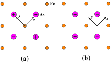
Figure 2: (color online) FeAs layer and specification of $(x,y,z)$. $xy$ plane consisting of Fe atoms is shown in (a) and (b) with different origin choices. $z$ axis is perpendicular to Fe-plane. “$+$”denotes an As atom above the Fe-plane, while “$-$”denotes an As atom below the Fe-plane. (a) Origin choice 1. (b) Origin choice 2. (also see Fig.1)

Table 5: Eight symmetry operations of $D_{2d}$ (an isomorphic group to $D_{4}$) will generate eight general positions. Where “general” is defined as the following: a set of symmetrical equivalent points is said to be in “general position” if each of its points is left invariant only by the identity operation but by no other symmetry operation of the space group. The origin choice is 1.

group element	general position
$E$	$\left(x,y,z\right)$
$C_{4z}\sigma_{h}$	$\left(y,-x,-z\right)$
$\left(C_{4z}\sigma_{h}\right)^{2}$	$\left(-x,-y,z\right)$
$\left(C_{4z}\sigma_{h}\right)^{3}$	$\left(-y,x,-z\right)$
$C_{2y}\sigma_{h}$	$\left(-x,y,z\right)$
$C_{2y}\sigma_{h}C_{4z}\sigma_{h}$	$\left(-y,-x,-z\right)$
$C_{2y}\sigma_{h}\left(C_{4z}\sigma_{h}\right)^{2}$	$\left(x,-y,z\right)$
$C_{2y}\sigma_{h}\left(C_{4z}\sigma_{h}\right)^{3}$	$\left(y,x,-z\right)$

Table 6: Four symmetry operations and corresponding general positions of group $I\times C_{2xy}$. The origin choice is 2.

group element	general position
$E$	$\left(x,y,z\right)$
$C_{i}$	$\left(-x,-y,-z\right)$
$C_{2xy}$	$\left(y,x,z\right)$
$C_{i}C_{2xy}$	$\left(-y,-x,-z\right)$

There are five irreducible representations of $D_{4}$ group, four of them, $A_{1}$, $A_{2}$, $B_{1}$ and $B_{2}$ are one-dimensional representations, and one of them, $E$ is a two-dimensional representation. All these five representations are representations of group $D_{4h}$ too. However, there are 2 two-dimensional irreducible representations $E^{\prime}$ and $E^{\prime\prime}$ of $D_{4h}$ group, neither of them is the representation of group $D_{4}$. Naively, $E^{\prime}$ and $E^{\prime\prime}$ can be viewed as subrepresentations of two irreducible representations of group $SU(2)$, $J=1/2$ and $J=3/2$, respectively. Since the representations $E^{\prime}$ and $E^{\prime\prime}$ can not result in quadratic terms in Hamiltonian or Ginzburg-Landau free energy, we will not discuss them in this paper.

Appendix C Transformation of gap functions

It is not $\Delta\left(\mathbf{k}\right)$ but $\psi\left(\mathbf{k}\right)$ and $\mathbf{d}\left(\mathbf{k}\right)$ transform as representations of symmetry group. In this appendix, we list the transformations of $\psi\left(\mathbf{k}\right)$ and $\mathbf{d}\left(\mathbf{k}\right)$ under various symmetry operations. Firstly, under a point-group transformation $g$, $\psi\left(\mathbf{k}\right)$ and $\mathbf{d}\left(\mathbf{k}\right)$ transform as

$$g\psi\left(\mathbf{k}\right) = \psi\left(D_{\left(G\right)}^{-}\left(g\right)\mathbf{k}\right),$$

$$g\mathbf{d}\left(\mathbf{k}\right) = D_{\left(G\right)}^{+}\left(g\right)\mathbf{d}\left(D_{\left(G\right)}^{-}\left(g\right)\mathbf{k}\right),$$ (11)

where $D_{\left(G\right)}^{\pm}\left(g\right)$ is the representation in three-dimensional space with positive (spin-space) or negative ($\mathbf{k}$-space) respectively. Secondly, time-reversal transformations of $\psi\left(\mathbf{k}\right)$ and $\mathbf{d}\left(\mathbf{k}\right)$ take the forms,

$$K\psi\left(\mathbf{k}\right)=\psi^{\ast}\left(-\mathbf{k}\right),K\mathbf{d}\left(\mathbf{k}\right)=-\mathbf{d}^{\ast}\left(-\mathbf{k}\right).$$ (12)

The anti-symmetric nature of Fermion systems, see Eq. (5), will lead to

$$\psi\left(-\mathbf{k}\right)=\psi\left(\mathbf{k}\right),\mathbf{d}\left(-\mathbf{k}\right)=-\mathbf{d}\left(\mathbf{k}\right),$$ (13)

for symmetric $\Omega$ and

$$\psi\left(-\mathbf{k}\right)=-\psi\left(\mathbf{k}\right),\mathbf{d}\left(-\mathbf{k}\right)=\mathbf{d}\left(\mathbf{k}\right),$$ (14)

for anti-symmetric $\Omega$. Hence, combining the above and the Hermitian choice of $\Omega$’s, the time-reversal invariance conditions for $\psi\left(\mathbf{k}\right)$ and $\mathbf{d}\left(\mathbf{k}\right)$ become

$$\psi^{\ast}\left(\mathbf{k}\right)=\psi\left(\mathbf{k}\right),\mathbf{d}^{\ast}\left(\mathbf{k}\right)=\mathbf{d}\left(\mathbf{k}\right),$$ (15)

since under time-reversal transformation, $\Omega$ transforms as

$$K\Omega=\Omega^{\ast}.$$ (16)

Appendix D Energy gap functions in the degenerate bands

The energy gap of the superconducting states indeed depends on the details of interaction, especially, depends on the ratio of $\delta t/\lambda$, where $\delta t$ is the energy scale of the splitting of two bands and $\lambda$ is the energy scale of pairing potential. In the the “strong pairing coupling” limit $\delta t\ll\lambda$, we expect the energy gap is close to $\delta t=0$ case, say, two bands are degenerate. A small perturbation proportional to $\delta t/\lambda$ will not change the energy gap very much, e.g. close the full gap or change from full gap to line nodal gap. In the weak pairing coupling limit $\lambda\ll\delta t$, the situation may be very different from strong coupling limit, which is discussed in Ref.QHWang . So that we will focus on the strong coupling limit and assume two degenerate bands in the following.

Due to two degenerate bands, the effective mean field Hamiltonian in $\mathbf{k}$-space can be written as an $8\times 8$ matrix,

$$\hat{H}_{\mathbf{k}}=\left(\begin{array}[]{cc}\xi_{\mathbf{k}}\sigma_{0}\otimes\sigma_{0}&\Delta(\mathbf{k})\\ \Delta^{{\dagger}}(\mathbf{k})&-\xi_{\mathbf{k}}\sigma_{0}\otimes\sigma_{0}\end{array}\right),$$ (17)

with the basis $\mathbf{c}_{\mathbf{k}}=(c_{\mathbf{k}\uparrow 1},c_{\mathbf{k}\uparrow 2},c_{\mathbf{k}\downarrow 1},c_{\mathbf{k}\downarrow 2},c_{-\mathbf{k}\uparrow 1}^{{\dagger}},c_{-\mathbf{k}\uparrow 2}^{{\dagger}},c_{-\mathbf{k}\downarrow 1}^{{\dagger}},c_{-\mathbf{k}\downarrow 2}^{{\dagger}})^{T}$. The indices in the $4\times 4$ matrices $\Delta(\mathbf{k})$ and $\xi_{\mathbf{k}}\sigma_{0}\otimes\sigma_{0}$ are arranged as the following, by direct products the former two indices denote spin space and the later two denote two orbitals. It is easy to know the energy dispersion,

$$E_{\mathbf{k}\mu}=\pm\sqrt{\xi_{\mathbf{k}}^{2}+\Delta_{\mathbf{k}\mu}^{2}},$$ (18)

where $\Delta_{\mathbf{k}\mu}^{2}$ is one of the eigenvalues of the matrix $\Delta(\mathbf{k})\Delta^{{\dagger}}(\mathbf{k})$. For degenerate bands, the minimum of $\left|\Delta_{\mathbf{k}\mu}\right|$ is the energy gap. For simplicity, we will focus on the $k_{z}$-independent pairing with a cylinder-like Fermi surface which is the case of doped $LaFeAsO$ most likely.

At first, we will consider the even parity, orbital anti-symmetric, spin triplet pairing states in Table II. Orbital anti-symmetric states have only one component $\sigma_{2}$ in the $\Omega$ part. Gap function is of the form, $\Delta(\mathbf{k})=i\left[\mathbf{\sigma}\cdot\mathbf{d}\left(\mathbf{k}\right)\right]\sigma_{2}\otimes\sigma_{2}$, thus $\Delta_{\mathbf{k}\mu}^{2}=\left|\mathbf{d}\right|^{2}\pm\left|\mathbf{d\times d}^{\ast}\right|$. For the time-reversal invariant state, $\mathbf{d}=\mathbf{d}^{\ast}$, the gapless condition follows as $\left|\mathbf{d}\right|^{2}=0$. For $B_{1g}$ and $B_{2g}$ states, they are $d$-wave states and have line nodal gap at Fermi surfaces. $A_{1g}$ states can be of either $s$-wave or extended $s$-wave. The $s$-wave state is of full gap while the extended $s$-wave state possibly has line nodal gap at Fermi surface, e.g., the state $\mathbf{d}\left(\mathbf{k}\right)=\cos k_{x}\cos k_{y}\hat{z}$. The $E_{g}$ representation involves $s$-wave, extended $s$-wave and $d$-wave states. The $s$-wave state is fully gapful, the $d$-wave state has line nodal gap, the extended $s$-wave state can be either fully gapful or of line nodal gap.

Then we consider the odd parity, orbital symmetric, spin triplet pairing states in Table IV. Orbital symmetric states have three components $\sigma_{0,1,3}$ in the $\Omega$ part. Gap function can be written as

$$\Delta(\mathbf{k})=i\left[\mathbf{\sigma}\cdot\mathbf{d}_{0}\left(\mathbf{k}\right)\right]\sigma_{2}\otimes\sigma_{0}+i\left[\mathbf{\sigma}\cdot\mathbf{d}_{1}\left(\mathbf{k}\right)\right]\sigma_{2}\otimes\sigma_{1}+i\left[\mathbf{\sigma}\cdot\mathbf{d}_{3}\left(\mathbf{k}\right)\right]\sigma_{2}\otimes\sigma_{3},$$ (19)

thus

$$\Delta(\mathbf{k})\Delta^{{\dagger}}(\mathbf{k}) = [(\left|\mathbf{d}_{0}\right|^{2}+\left|\mathbf{d}_{1}\right|^{2}+\left|\mathbf{d}_{3}\right|^{2})\sigma_{0}+i\left(\mathbf{d}_{0}\mathbf{\times d}_{0}^{\ast}+\mathbf{d}_{1}\mathbf{\times d}_{1}^{\ast}+\mathbf{d}_{3}\mathbf{\times d}_{3}^{\ast}\right)\cdot\mathbf{\sigma}]\otimes\sigma_{0}$$ (20)

$$+\left[\left(\mathbf{d}_{0}\cdot\mathbf{d}_{1}^{\ast}+\mathbf{d}_{1}\cdot\mathbf{d}_{0}^{\ast}\right)\sigma_{0}+i\left(\mathbf{d}_{0}\mathbf{\times d}_{1}^{\ast}+\mathbf{d}_{1}\mathbf{\times d}_{0}^{\ast}\right)\cdot\mathbf{\sigma}\right]\otimes\sigma_{1}$$

$$+\left[\left(\mathbf{d}_{0}\cdot\mathbf{d}_{3}^{\ast}+\mathbf{d}_{3}\cdot\mathbf{d}_{0}^{\ast}\right)\sigma_{0}+i\left(\mathbf{d}_{0}\mathbf{\times d}_{3}^{\ast}+\mathbf{d}_{3}\mathbf{\times d}_{0}^{\ast}\right)\cdot\mathbf{\sigma}\right]\otimes\sigma_{3}$$

$$+\left[\left(\mathbf{d}_{1}\mathbf{\times d}_{3}^{\ast}-\mathbf{d}_{3}\mathbf{\times d}_{1}^{\ast}\right)\cdot\mathbf{\sigma}-i\left(\mathbf{d}_{1}\cdot\mathbf{d}_{3}^{\ast}-\mathbf{d}_{3}\cdot\mathbf{d}_{1}^{\ast}\right)\sigma_{0}\right]\otimes\sigma_{2}.$$

For a time-reversal invariant state, $\mathbf{d}_{i}^{\ast}\left(\mathbf{k}\right)=\mathbf{d}_{i}\left(\mathbf{k}\right)$, $i=0,1,3$, so that the above can be simplified as

$$\Delta(\mathbf{k})\Delta^{{\dagger}}(\mathbf{k})=\left(\mathbf{d}_{0}^{2}+\mathbf{d}_{1}^{2}+\mathbf{d}_{3}^{2}\right)\sigma_{0}\otimes\sigma_{0}+2\left(\mathbf{d}_{0}\cdot\mathbf{d}_{1}\right)\sigma_{0}\otimes\sigma_{1}+2\left(\mathbf{d}_{0}\cdot\mathbf{d}_{3}\right)\sigma_{0}\otimes\sigma_{3}+2\left(\mathbf{d}_{1}\mathbf{\times d}_{3}\right)\cdot\mathbf{\sigma}\otimes\sigma_{2}.$$ (21)

We obtain from the above

$$\Delta_{\mathbf{k}\mu}^{2}=\left(\mathbf{d}_{0}^{2}+\mathbf{d}_{1}^{2}+\mathbf{d}_{3}^{2}\right)\pm 2\sqrt{\left(\mathbf{d}_{0}\cdot\mathbf{d}_{1}\right)^{2}+\left(\mathbf{d}_{0}\cdot\mathbf{d}_{3}\right)^{2}+\left(\mathbf{d}_{1}\mathbf{\times d}_{3}\right)^{2}}.$$ (22)

Gapless condition reads

$$\mathbf{d}_{0}^{2}+\mathbf{d}_{1}^{2}+\mathbf{d}_{3}^{2}=2\sqrt{\left(\mathbf{d}_{0}\cdot\mathbf{d}_{1}\right)^{2}+\left(\mathbf{d}_{0}\cdot\mathbf{d}_{3}\right)^{2}+\left(\mathbf{d}_{1}\mathbf{\times d}_{3}\right)^{2}}.$$ (23)

Careful analysis shows node can appear only when at least one of $\left|\mathbf{d}_{0}\right|$, $\left|\mathbf{d}_{1}\right|$ and $\left|\mathbf{d}_{3}\right|$ vanish. So that $E_{u}$ states in Table IV are of line nodal gap. The other four representations $A_{1u}$, $A_{2u}$, $B_{1u}$ and $B_{2u}$ can be of either line nodal or full gap. For example, for an $A_{1u}$ states in Table IV which consists of two components in the $\Omega$ part, $\mathbf{d}_{0}\left(\mathbf{k}\right)=\sin k_{x}\hat{x}+\sin k_{y}\hat{y}$, $\mathbf{d}_{3}\left(\mathbf{k}\right)=\sin k_{x}\hat{x}-\sin k_{y}\hat{y}$ and $\mathbf{d}_{1}\left(\mathbf{k}\right)=0$, nodal lines will appear at $\sin k_{x}=0$ and $\sin k_{y}=0$. Moreover, any $A_{1u}$ state in Table IV which consists of only one component in the $\Omega$ part is of full gap.

Similar consideration will lead to the results for spin singlet states shown in Tables I and III. Of course, when the ratio $\delta t/\lambda$ becomes large, the situation may change. This change strongly depends on the details of both pairing states and the Hamiltonian. For example, for an $s$-wave with $\mathbf{d}\left(\mathbf{k}\right)=\hat{z}$, and $\Omega=\sigma_{2}$, Fermi pockets may appear when $\delta t$ and $\lambda$ are comparable.

References

• (1) M. Sigrist and K. Ueda, Rev. Mod. Phys. 63, 239 (1991).
• (2) Y. Kamihara, T. Watanabe, M. Hirano, H. Hosono, J. Am. Chem. Soc. 130, 3296 (2008); H. Takahashi, K. Igawa, K. Arii, Y. Kamihara, M. Hirano, H. Hosono, Nature, 453, 376 (2008).
• (3) G. F. Chen, Z. Li, D. Wu, G. Li, W. Z. Hu, J. Dong, P. Zheng, J. L. Luo, and N. L. Wang, Phys. Rev. Lett. 100, 247002 (2008).
• (4) X. H. Chen, T. Wu, G. Wu, R. H. Liu, H. Chen and D. F. Fang, Nature, 453, 761 (2008).
• (5) Z. A. Ren, J. Yang, W. Lu, W. Yi, G. C. Che, X. L. Dong, L. L. Sun, Z. X. Zhao, Mater. Res. Innovations 12, 1 (2008).
• (6) Z. A. Ren, W. Lu, J. Yang, W. Yi, X. L. Shen, Z. C. Li, G. C. Che, X. L. Dong, L. L. Sun, F. Zhou and Z. X. Zhao, Chin. Phys. Lett. 25, 2215 (2008).
• (7) C. Wang, L. J. Li, S. Chi, Z. W. Zhu, Z. Ren, Y. K. Li, Y. T. Wang, X. Lin, Y. K. Luo, X. F. Xu, G. H. Cao and Z. A. Xu, arxiv:0804.4290 (2008).
• (8) Z. A. Ren, G. C. Che, X. L. Dong, J. Yang, W. Lu, W. Yi, X. L. Shen, Z. C. Li, L. L. Sun, F. Zhou and Z. X. Zhao, Europhys. Lett. 83 17002 (2008).
• (9) H. H. Wen, G. Mu, L. Fang, H. Yang and X. Y. Zhu, Europhys. Lett. 82, 17009 (2008).
• (10) J. Dong, H. J. Zhang, G. Xu, Z. Li, G. Li, W. Z. Hu, D. Wu, G. F. Chen, X. Dai, J. L. Luo, Z. Fang and N. L. Wang, Europhys. Lett. 83, 27006 (2008).
• (11) Clarina de la Cruz, Q. Huang, J. W. Lynn, J. Y. Li, W. Ratcliff II, J. L. Zarestky, H. A. Mook, G. F. Chen, J. L. Luo, N. L. Wang and P. C. Dai, Nature 453, 899 (2008).
• (12) G. Mu, X. Zhu, L. Fang, L. Shan, C. Ren and H. H. Wen, Chin. Phys. Lett. 25, 2221 (2008).
• (13) K. Ahilan, F. L. Ning, T. Imai, A. S. Sefat, R. Jin, M. A. McGuire, B. C. Sales and D. Mandrus, arxiv:0804.4026 (2008).
• (14) Y. Nakai, K. Ishida, Y. Kamihara, M. Hirano, H. Hosono, J. Phys. Soc. Jpn. 77 073701 (2008).
• (15) K. Matano, Z. A. Ren, X. L. Dong, L. L. Sun, Z. X. Zhao, G. Q. Zheng, Europhys. Lett. 83, 57001 (2008).
• (16) L. Boeri, O. V. Dolgov, A. A. Golubov, Phy. Rev. Lett. 101, 026403 (2008).
• (17) D. J. Singh and M. H. Du, Phys. Rev. Lett. 100, 237003 (2008).
• (18) K. Haule, J. H. Shim and G. Kotliar, Phys. Rev. Lett. 100, 226402 (2008).
• (19) G. Xu, W. Ming, Y. Yao, X. Dai, S. C. Zhang and Z. Fang, Europhys. Lett. 82, 67002 (2008).
• (20) I. I. Mazin, D. J. Singh, M. D. Johannes and M. H. Du, Phys. Rev. Lett. 101, 057003 (2008).
• (21) C. Cao, P. J. Hirschfeld and H. P. Cheng, Phys. Rev. B77, 220506(R) (2008).
• (22) F. J. Ma and Z. Y. Lu, Phys. Rev. B 78, 033111 (2008).
• (23) X. Dai, Z. Fang, Y. Zhou. F. C. Zhang, Phys. Rev. Lett. 101, 057008 (2008)
• (24) T. Li, arXiv:0804.0536 (2008).
• (25) P. A. Lee and X. G. Wen, arxiv:0804.1739 (2008).
• (26) Z. Y. Weng, arXiv:0804.3228 (2008)
• (27) S. Raghu, X. L. Qi, C. X. Liu, D. J. Scalapino, S. C. Zhang, Phys. Rev. B77, 220503(R) (2008).
• (28) Z. J. Yao, J. X. Li and Z. D. Wang, arxiv:0804.4166 (2008).
• (29) Q. M. Si and E. Abrahams , arxiv:0804.2480, Phys. Rev. Lett. (to be published)
• (30) T. A. Maier, D. J. Scalapino, arxiv:0805.0316 (2008).
• (31) International tables for crystallography, Volume A, Space-Group Symmetry, 4th Edition, Kluwer Academic Publishers, Dordrecht, Nertherlands (1996).
• (32) If the lattice undergoes a structural transition, e.g., the transition from tetragonal ($P4/nmm$) to monoclinic ($P112/n$) in the parent compound L​a​F​e​A​s​OπΏπ‘ŽπΉπ‘’π΄π‘ π‘‚LaFeAsO, lattice symmetry will be reduced and thereby the pairing states within each representation of $D_{4}$ will be further splitted by energy. However, Ps​p​a​c​esubscriptπ‘ƒπ‘ π‘π‘Žπ‘π‘’P_{space}, $P_{spin}$ and $P_{orbital}$ considered in this paper are still good quantum numbers. Moreover, when the monoclinic distortion to tetragonal phase is small as in practice,Neutron our study is a good approximation to such a monoclinic lattice.
• (33) P. H. Butler, Point Group Symmetry Applications: Methods and Tables, Plenum Press, New York (1981).
• (34) Z. H. Wang, H. Tang, Z. Fang and X. Dai, arXiv:0805.0736 (2008).
• (35) M. Daghofer, A. Moreo, J. A. Riera, E. Arrigoni and E. Dagotto, arXiv:0805.0148 (2008).
• (36) Y. Wan and Q. H. Wang, arXiv:0805.0923 (2008).
• (37) J. R. Shi, arXiv:0806.0259 (2008).