A path integral approach to closed-form option pricing formulas with applications to stochastic volatility and interest rate models

Abstract

We present a path integral method to derive closed-form solutions for option prices in a stochastic volatility model. The method is explained in detail for the pricing of a plain vanilla option. The flexibility of our approach is demonstrated by extending the realm of closed-form option price formulas to the case where both the volatility and interest rates are stochastic. This flexibility is promising for the treatment of exotic options. Our new analytical formulas are tested with numerical Monte Carlo simulations.

I Introduction

Since the seminal work of Black and Scholes BlackScholes ; MERT , who drew an analogy between the random motion of microscopic particles and the unpredictable evolution of stock prices, methods from theoretical physics have proved very useful for pricing various financial derivative products baaquiebook ; kleinertbook ; Dashb . The pricing of derivative products is based on a model for the evolution of the probability function of the underlying asset. In order for a model to describe the economic reality accurately, a sufficiently general evolution for the probability distribution has to be allowed for. Nevertheless, the simple diffusion model of Black and Scholes (BS) is still widely used. Much of its success is due to the availability of closed-form analytical pricing formulas for many types of derivatives wilmott .

It is known for a long time that the BS model is only a crude approximation to the economic reality and that its assumptions are violated in actual markets. Perhaps the most illustrative violation is that the volatility implied from traded vanilla options, the implied volatility is not constant across strikes and maturities. Examples of models that tackle such violations are local volatility processes Rcont ; Derman , jump processes Rcont , Lévy processes Schoutens and stochastic volatility models Lipton . A stochastic volatility model that has been particularly successful at explaining the implied volatility smile in equity and foreign exchange markets is the Heston model Heston . In his seminal paper, Heston Heston derived a closed form solution for the price of a vanilla option, which enables a quick and reliable calibration to market prices, especially for liquidly traded vanilla options with maturities between 2 months and 2 years Cizek . Contrary to the Black-Scholes model, to date in the Heston model no closed-form analytic formulas have been found for exotic options (for recent results see Griebsch ). Since no such formulas are available in the literature for any but the simplest payoffs, often costly numerical techniques have to be used (see Anders and references therein).

The original mathematical solution of the option pricing problem was formulated within the framework of partial differential equations, but an equivalent description with path integral methods was developed in the pioneering work by Linetsky Linetsky and Dash Dash ; DashII . They showed that path dependent exotic options can be straightforwardly priced with the path integral method. This should be intuitively clear: in the path integral formalism, a probability is assigned to every evolution path of the asset. In the formulation with partial differential equations, such quantities are typically difficult to access.

Path integral methods have also been used in the pricing of options within stochastic volatility models baaquieJP ; Dragu and in the related problem of non-Gaussian diffusion KleinertPhysA (at the end of Sec. II.1 we come back to this connection), but to the best of our knowledge no explicit option pricing formula as cheap to evaluate as Stein and Stein’s Stein or Heston’s formulas Heston have yet been derived using path integrals. We will show in the present paper how to carry out this task for the Heston model. The result we thereby obtain corresponds to the existing result Heston for which the calibration and correspondence to market data has already been investigated see for example drag2 ; drag3 ; jap2 ; Yacine ; Fior ; Ranjan . For a thorough discussion on when which approach should be used we refer to Rebon and references herein.

It is also known that there are still important features of asset price distributions which are absent in the Heston model for example: empirical studies of time series provide evidence of the long time memory of volatility Bouch ; Gop . Since models containing a memory effect through retarded interaction, for example in the context of polarons, FM , have been solved within a path integral framework, we think our method can prove to be useful in more realistic models for the market also.

The full power of the path integral method becomes clear, when we exploit its flexibility by calculating the price of an option in a setting where not only the volatility but also the interest rate is stochastic and follows the widely used CIR model cir ; Brown ; Gibbon ; Dsev . To the best of our knowledge, no exact closed-form formula for this problem is available. Therefore, we have checked our formulas against a Monte Carlo simulation.

The plan of the paper is as follows. In Sec. II.1, we outline our model, which is the one introduced by Heston. Extensions of our method to different models are however straightforward. Further in this section we derive a closed-form solution for the time evolution of the asset price. In Sec. II.2 we present a closed-form pricing formula for plain vanilla options which only involves one numerical integration of a compilation of elementary functions. In Sec. III we will extend the Heston model to include stochastic interest rate, in Sec. III A we present a closed-form solution for the vanilla option price which still contains only on numerical integration of a compilation of elementary functions. In Sec. III.2 we test this result with a Monte Carlo method and discuss the relevance of including stochastic interest rate. Conclusions are drawn in Sec. IV.

II Standard Heston model

II.1 The model and its path integral representation

We will concentrate on assets following a diffusion process described by the following two equations introduced by Heston Heston

$$dS =\mu_{0}Sdt+S\sqrt{v}dw_{1},$$ (1)

$$dv =\kappa_{0}\left(\theta_{0}-v\right)dt+\sigma\sqrt{v}\left(\rho dw_{1}+\sqrt{1-\rho^{2}}dw_{2}\right).$$ (2)

Here $S$ is the asset price, $\mu_{0}$ is a constant drift factor, $v$ is the variance of the asset, $\kappa_{0}$ is the spring constant of the force that attracts the variance to its mean reversion level $\theta_{0}$(also called the mean reversion speed), $\sigma$ is the volatility of the variance, and $w_{1}$ and $w_{2}$ are independent Wiener processes with unit variance and zero mean. The asset price follows a Black-Scholes process BlackScholes , whereas the volatility obeys a Cox-Ingersoll-Ross process cir .

There are two general approaches to determine the price of an option in a path integral context. One could, based upon equations (1), (2) determine the probability distribution for the asset price at the strike time $T$ conditional on the values of the asset and the variance at the present time $P_{S}\left(S_{T},v_{T}\mid S_{0},v_{0}\right)$. The expectation value of the option price at time $T$ can be calculated by integrating the gain you make with a certain outcome of $S_{T}$ multiplied by the probability of obtaining that outcome $P_{S}\left(S_{T},v_{T}\mid S_{0},v_{0}\right)$ over all possible values of $S_{T}$. To obtain the present value of the price one then discounts this expectation value with the risk free interest rate $r$. For a European call option this can be written as:

$$\mathcal{C}=e^{-rT}\int\limits_{-\infty}^{+\infty}dS_{T}dv_{T}\max\left[S_{T}-K,0\right]P_{S}\left(S_{T},v_{T}\mid S_{0},v_{0}\right).$$ (3)

We will refer to this approach as the ”asset propagation approach” since $P_{S}$ is the propagator for a distribution of asset prices (and volatilities).

The other approach focuses on the option price rather than the asset evolution, as will be referred to as the ”option propagation approach”. In his paper [6], Heston discusses the subtle differences between the asset point of view and the option price point of view, and this discussion is also relevant to the present path-integral framework. Heston motivates that the time evolution of the option price $U\left(S,v,t\right)$ is governed by the following partial differential equation (pde):

$$\frac{\partial U}{\partial t}=-rS\frac{\partial U}{\partial S}+rU-\left\{\kappa_{0}\left[\theta_{0}-v\right]-\lambda v\right\}\frac{\partial U}{\partial v}-\frac{1}{2}vS^{2}\frac{\partial^{2}U}{\partial S^{2}}-\rho\sigma vS\frac{\partial^{2}U}{\partial S\partial v}-\frac{1}{2}\sigma^{2}v\frac{\partial^{2}U}{\partial v^{2}},$$ (4)

where $\lambda$ is a parameter introduced Heston on the basis of no-arbritage arguments and setting up a risk-free portfolio. If one makes the substitution $U=e^{rt}V$  one obtains the following pde for $V$ as a function of the asset price and the volatility:

$$\frac{\partial V}{\partial t}=-rS\frac{\partial V}{\partial S}-\left\{\kappa_{0}\left[\theta_{0}-v\right]-\lambda v\right\}\frac{\partial V}{\partial v}-\frac{1}{2}vS^{2}\frac{\partial^{2}V}{\partial S^{2}}-\rho\sigma vS\frac{\partial^{2}V}{\partial S\partial v}-\frac{1}{2}\sigma^{2}v\frac{\partial^{2}V}{\partial v^{2}}.$$ (5)

Based on this pde, one can find a kernel $P_{V}$  that propagates a given final distribution $V\left(S_{T},v,T\right)$ backwards to the present value $V(S_{0},v_{0},0)$ of the option. Since the value of the option at the final time $T$ is known, $V\left(S_{T},v,T\right)=e^{-rT}U\left(S_{T},v,T\right)=e^{-rT}\max\left[S_{T}-K,0\right]$, the value of the option now is obtained through

$$\mathcal{C}=e^{-rT}\int\limits_{-\infty}^{+\infty}dS_{T}dv_{T}\max\left[S_{T}-K,0\right]P_{V}\left(S_{T},v_{T}\mid S_{0},v_{0}\right),$$ (6)

Furthermore the pde (5) is equal to the Kolmogorov backward equation corresponding to the following system of stochastic differential equations

$$dS =rSdt+S\sqrt{v}dw_{1},$$ (7)

$$dv =\left\{\kappa_{0}\left[\theta_{0}-v\right]-\lambda v\right\}dt+\sigma\sqrt{v}\left(\rho dw_{1}+\sqrt{1-\rho^{2}}dw_{2}\right).$$ (8)

This means that both approaches can be dealt with simultaneously by considering a generalized stochastic process:

$$dS =\mu Sdt+S\sqrt{v}dw_{1},$$ (9)

$$dv =\kappa\left(\theta-v\right)dt+\sigma\sqrt{v}\left(\rho dw_{1}+\sqrt{1-\rho^{2}}dw_{2}\right).$$ (10)

and calculating its transition probability $P\left(S_{T},v_{T}\mid S_{0},v_{0}\right)$. The ”asset propagation” approach (3) can then be retained by simply replacing $\mu,\kappa$ and $\theta$ by $\mu_{0},\kappa_{0}$ and $\theta_{0}$ and the ”option propagation” approach (5), (6) by replacing $\mu,\kappa$ and $\theta$ by $r,\kappa_{0}+\lambda$ and $\kappa_{0}\theta_{0}/\left(\kappa_{0}+\lambda\right)$. The pricing formula for the European call is the same as (3) where this time the transition probability $P\left(S_{T},v_{T}\mid S_{0},v_{0}\right)$ is the one corresponding to (9), (10):

$$\left\{\begin{array}[c]{l}P_{S}\left(S_{T},v_{T}\mid S_{0},v_{0}\right)=\left.P\left(S_{T},v_{T}\mid S_{0},v_{0}\right)\right|_{\mu=\mu_{0},\kappa=\kappa_{0},\theta=\theta_{0}}\\ P_{V}\left(S_{T},v_{T}\mid S_{0},v_{0}\right)=\left.P\left(S_{T},v_{T}\mid S_{0},v_{0}\right)\right|_{\mu=r,\kappa=\kappa_{0}+\lambda,\theta=\kappa_{0}\theta_{0}/(\kappa_{0}+\lambda)}\end{array}\right.$$ (11)

We will calculate the transition density $P$ for the general stochastic process (9), (10).

For later convenience we make the following substitutions:

$$x =\ln\left(\frac{S}{S_{0}}\right)-\mu t,$$ (12)

$$z =\sqrt{v},$$

$x$ is called the logreturn and $z$ is the volatility of the asset price. After these substitutions, Eq. (2) becomes:

$$dx =-\frac{z^{2}}{2}dt+zdw_{1},$$ (13)

$$dz =\left[\frac{1}{2z}\left(\kappa\theta-\frac{\sigma^{2}}{4}\right)-\kappa\frac{z}{2}\right]dt+\frac{\sigma}{2}\left(\rho dw_{1}+\sqrt{1-\rho^{2}}dw_{2}\right).$$ (14)

The substitution

$$y\left(t\right)=x\left(t\right)-\frac{\rho}{\sigma}\left(z^{2}\left(t\right)-\kappa\theta t\right),$$

leads to two uncorrelated equations:

$$dy =\left(\frac{\rho}{\sigma}\kappa-\frac{1}{2}\right)z^{2}dt+z\sqrt{1-\rho^{2}}dw_{1},$$ (15)

$$dz =\left[\frac{1}{2z}\left(\kappa\theta-\frac{\sigma^{2}}{4}\right)-\kappa\frac{z}{2}\right]dt+\frac{\sigma}{2}dw_{2}.$$ (16)

We will assume that the initial volatility $z(t=0)=z_{0}$ is known Cizek . The probability that $y$ has the value $y_{T}$ and $z$ the value $z_{T}$ at a later time $T$ will be denoted as $P\left(y_{T},z_{T}\mid y_{0},z_{0}\right)$. The advantage of transforming to these variables is that $dw_{1}$ and $dw_{2}$ are uncorrelated, so that the following expression holds for $P\left(y_{T},z_{T}\mid y_{0},z_{0}\right)$:

$$P\left(y_{T},z_{T}\mid y_{0},z_{0}\right)=\int\mathcal{D}y\mathcal{D}z\exp\left(-\int\limits_{0}^{T}\left\{\mathcal{L}_{Q}\left[y(t),z(t)\right]+\mathcal{L}_{CIR}[z(t)]\right\}dt\right).$$ (17)

Where the quadratic Lagrangian $\mathcal{L}_{Q}\left(y(t),z(t)\right)$ equals

$$\mathcal{L}_{Q}\left(y(t),z(t)\right)=\frac{1}{2z^{2}\left(1-\rho^{2}\right)}\left[\dot{y}-\left(\frac{\rho}{\sigma}\kappa-\frac{1}{2}\right)z^{2}\right]^{2},$$ (18)

and the Lagrangian corresponding to the CIR process, $\mathcal{L}_{CIR}[z(t)]$, is given by Rosa :

$$\mathcal{L}_{CIR}[z]=\frac{2}{\sigma^{2}}\left\{\dot{z}-\frac{1}{2}\left[\frac{1}{z}\left(\kappa\theta-\frac{\sigma^{2}}{4}\right)-\kappa z\right]\right\}^{2}-\frac{1}{4z^{2}}\left(\kappa\theta-\frac{\sigma^{2}}{4}\right)-\frac{\kappa}{4},$$ (19)

The first step in the evaluation of Eq. (17) is the integration over all $y$-paths. Because the action is quadratic in $y$ this integration can be done analytically and yields

$$P\left(y_{T},z_{T}\mid y_{0},z_{0}\right) =\int\mathcal{D}z(t)\frac{1}{\sqrt{2\pi\bar{z}^{2}\left(1-\rho^{2}\right)}}\exp\left\{\frac{\left(\frac{\rho}{\sigma}\kappa-\frac{1}{2}\right)}{\left(1-\rho^{2}\right)}\left(y_{T}-y_{0}\right)\right.$$

$$-\frac{1}{2\left(1-\rho^{2}\right)}\left(\frac{\rho}{\sigma}\kappa-\frac{1}{2}\right)^{2}\bar{z}^{2}-\frac{\left(y_{T}-y_{0}\right)^{2}}{2\bar{z}^{2}\left(1-\rho^{2}\right)}$$

$$\left.-\int_{0}^{T}dt\text{ }\mathcal{L}_{CIR}[z(t)]\right\}.$$ (20)

Note that the probability to arrive in $(y_{T},z_{T})$ only depends on the average value of the volatility along the path $z(t)$: $\bar{z}^{2}=\int_{0}^{T}z^{2}(t)dt$, in agreement with Ref. Stein . However, this average value appears in the denominator of the third term, and to perform the functional integral one needs to bring this into the numerator. This is achieved by rewriting part of the expression (20) as follows:

$$\frac{1}{\sqrt{2\pi\bar{z}^{2}\left(1-\rho^{2}\right)}}\exp\left[-\frac{\left(y_{T}-y_{0}\right)^{2}}{2\bar{z}^{2}\left(1-\rho^{2}\right)}\right]=\int_{-\infty}^{+\infty}\frac{dk}{2\pi}\exp\left[i\left(y_{T}-y_{0}\right)k-\frac{\int z^{2}dt\left(1-\rho^{2}\right)}{2}k^{2}\right].$$ (21)

Combining Eqns. (20) and (21) and making the substitution $k=l+i\frac{\left(\frac{\rho}{\sigma}\kappa-\frac{1}{2}\right)}{\left(1-\rho^{2}\right)}$ the transition probability becomes

$$P\left(y_{T},z_{T}\mid y_{0},z_{0}\right) =\int_{-\infty}^{+\infty}\frac{dl}{2\pi}\exp\left[i\left(y_{T}-y_{0}\right)l\right]\int\mathcal{D}z(t)$$ (22)

$$\times \exp\left(-\int_{0}^{T}dt\left\{\mathcal{L}_{CIR}[z(t)]+\frac{1}{2}z^{2}\left[\left(1-\rho^{2}\right)l^{2}+2li\left(\frac{\rho}{\sigma}\kappa-\frac{1}{2}\right)\right]\right\}\right).$$

The path integral over the CIR action is formally equivalent to the exactly solvable radial harmonic oscillator GenS and, fortunately, adding terms proportional to $z^{2}$ to the action does not spoil this equivalence. The full path integral over $z(t)$ can be carried out without approximations with the following result:

$$P\left(y_{T},z_{T}\mid y_{0},z_{0}\right) =\frac{1}{2\pi}\exp\left[\frac{\kappa^{2}\theta}{\sigma^{2}}T+\left(2\frac{\kappa\theta}{\sigma^{2}}-\frac{1}{2}\right)\ln\left(\frac{z_{T}}{z_{0}}\right)-\frac{\kappa}{\sigma^{2}}\left(z_{T}^{2}-z_{0}^{2}\right)\right]$$

$$\times \int\limits_{-\infty}^{+\infty}\exp\left[i\left(y_{T}-y_{0}\right)l\right]\sqrt{z_{0}z_{T}}\frac{4\omega}{\sigma^{2}\sinh\left(\omega T\right)}$$

$$\times \exp\left[-\frac{2\omega}{\sigma^{2}}\left(z_{0}^{2}+z_{T}^{2}\right)\coth\left(\omega T\right)\right]I_{\frac{2}{\sigma^{2}}\kappa\theta-1}\left[\frac{4\omega z_{0}z_{T}}{\sigma^{2}\sinh\left(\omega T\right)}\right]dl.$$ (23)

where

$$\omega=\frac{\sigma}{2}\sqrt{\left(\frac{\kappa}{\sigma}+il\rho\right)^{2}+l\left(l-i\right)}.$$ (24)

is the $l$-dependent frequency of the radial harmonic oscillator that corresponds to the CIR Lagrangian (19). After transforming back to the $x$ variable we see that also the integral over the final value $z_{T}$ can be done analytically (see e.g. Prudni ), yielding the marginal probability distribution $\mathcal{P}\left(x_{T}\mid 0,z_{0}\right)=\int_{-\infty}^{+\infty}dz_{T}P\left(x_{T},z_{T}\mid 0,z_{0}\right)$ (written in the original variable $v$) as a simple Fourier integral:

$$\mathcal{P}\left(x_{T}\mid 0,v_{0}\right) =\frac{1}{2\pi}\exp\left[\frac{\kappa}{\sigma^{2}}\left(\kappa\theta T+v_{0}\right)\right]$$

$$\times\int\limits_{-\infty}^{+\infty}N^{\frac{2}{\sigma^{2}}\kappa\theta}\exp\left\{i\left[x_{T}+\frac{\rho}{\sigma}\left(v_{0}+\kappa\theta T\right)\right]l\right.$$

$$\left.-\frac{2\omega}{\sigma^{2}\sinh\left(\omega T\right)}\left[\cosh\left(\omega T\right)-N\right]v_{0}\right\}dl,$$ (25)

where N is:

$$N=\frac{1}{\cosh\left(\omega T\right)+\frac{1}{2\omega}\left(\kappa+il\rho\sigma\right)\sinh\left(\omega T\right)}.$$ (26)

Note the similarity of the expression (25) with the result obtained in Ref. KleinertPhysA , derived for a general stochastic process with non-Gaussian noise.

II.2 Pricing of plain vanilla options

From now on we follow the option propagation approach and set $\mu$ equal to $r$. The price of a call option $\mathcal{C}$ with expiration date $T$ and strike $K$ when the transition probability is known is given by Eq. (3). Writing this formula in the $x$ variable and thereby inserting the result (25) for the transition probability results in:

$$\mathcal{C}=e^{-rT}\int\limits_{-\infty}^{+\infty}dx_{T}\max\left[S_{0}\exp\left(x_{T}\right)-K,0\right]\mathcal{P}\left(x_{T}\mid 0,v_{0}\right),$$ (27)

where the risk free interest rate was restored and denoted by $r$. Now there are still two numerical integrations that have to be done. Following the derivation outlined in Ref. KleinertPhysA  we can rewrite expression (27) so that only one numerical integration remains:

$$\mathcal{C} =\frac{S_{0}-e^{-rT}K}{2}+i\int\limits_{-\infty}^{\infty}\frac{1}{l}\left\{\exp\left[i\left(\frac{\rho}{\sigma}a+x_{e}-rT\right)l+\frac{\kappa}{\sigma^{2}}a\right]\right.$$ (28)

$$\left.\times\left[S_{0}\exp\left(\Theta-\frac{\rho}{\sigma}a\right)-e^{-rT}K\exp\left(\Upsilon\right)\right]-S_{0}+e^{-rT}K\right\}\frac{dl}{2\pi},$$

with

$$x_{e} =\ln\left(\frac{K}{S_{0}}\right),$$ (29a)

$$a =v_{0}+\kappa\theta T,$$ (29b)

$$\nu =\frac{\sigma}{2}\sqrt{\left(\frac{\kappa}{\sigma}+il\rho-\rho\right)^{2}+l\left(l+i\right)},$$ (29c)

$$M =\left[\cosh\left(\nu T\right)+\frac{1}{2\nu}\left(\kappa+il\rho\sigma-\rho\sigma\right)\sinh\left(\nu T\right)\right]^{-1},$$ (29d)

$$\Theta =\frac{2\nu v_{0}}{\sigma^{2}\sinh\left(\nu T\right)}\left[M-\cosh\left(\nu T\right)\right]+\frac{2}{\sigma^{2}}\kappa\theta\log M,$$ (29e)

$$\Upsilon =\frac{2\omega v_{0}}{\sigma^{2}\sinh\left(\omega T\right)}\left[N-\cosh\left(\omega T\right)\right]+\frac{2}{\sigma^{2}}\kappa\theta\log N.$$ (29f)

and $$\omega$$ defined as before (24). We have tested this result against the formula stated in Ref. Heston . This confirmed the correctness of formula (28). Now we are confident to explore new grounds with our method in the following section.

III Stochastic interest rate

III.1 Derivation of the option price

In the previous section we assumed the interest rate to be constant. Here we allow the interest rate to change in time, $r(t)$. Applying Black and Scholes’ no-arbitrage argument on Heston’s risk-free portfolio motivation for the evolution of the option price, we again obtain the partial differential equation (5) with $r(t)$ rather than a constant $r:$

$$\frac{\partial V}{\partial t}=-r(t)S\frac{\partial V}{\partial S}-\left\{\kappa_{0}\left[\theta_{0}-v\right]-\lambda v\right\}\frac{\partial V}{\partial v}-\frac{1}{2}vS^{2}\frac{\partial^{2}V}{\partial S^{2}}-\rho\sigma vS\frac{\partial^{2}V}{\partial S\partial v}-\frac{1}{2}\sigma^{2}v\frac{\partial^{2}V}{\partial v^{2}}$$ (30)

For a given function $r(t)$ this leads to a kernel $P_{V}\left[S_{T},v_{T}\mid S_{0},v_{0}\mid r(t)\right]$ so that the option price becomes

$$\mathcal{C}[r(t)]=\int\limits_{-\infty}^{+\infty}dS_{T}dv_{T}\max\left[S_{T}-K,0\right]\text{ }e^{-\int r(t)dt}P_{V}\left[S_{T},v_{T}\mid S_{0},v_{0}\mid r(t)\right].$$ (31)

Note that the option price is now a functional of the given time evolution of the interest rate $r(t)$. As in the previous section, it is convenient to introduce new integration variables

$$y\left(t\right) =\ln\left(\frac{S}{S_{0}}\right)-\frac{\rho}{\sigma}\left[z^{2}\left(t\right)-\kappa\theta t\right],$$ (32)

$$z(t) =\sqrt{v(t)}.$$ (33)

In the path-integral treatment, the kernel can be written as a sum over all possible realizations of $y(t)$ and $z(t)$, weighed by the action functional of the system:

$$\mathcal{C}[r(t)] =\int\limits_{-\infty}^{+\infty}dx_{T}dv_{T}\max\left[e^{x_{T}}-K,0\right]\text{ }e^{-{\textstyle\int\nolimits_{0}^{T}}r(t)dt}$$

$$\times\int\mathcal{D}y\mathcal{D}z\text{ }\exp\left(-\int\limits_{0}^{T}\left\{\mathcal{L}_{Q}\left[y(t),z(t),r(t)\right]+\mathcal{L}_{CIR}[z(t)]\right\}dt\right),$$ (34)

where $\mathcal{L}_{Q}$ is the quadratic Lagrangian (18)

$$\mathcal{L}_{Q}\left(y(t),z(t)\right)=\frac{1}{2z^{2}\left(1-\rho^{2}\right)}\left[\dot{y}(t)-r(t)-\left(\frac{\rho}{\sigma}\kappa-\frac{1}{2}\right)z^{2}(t)\right]^{2},$$ (35)

and $\mathcal{L}_{CIR}$ is the CIR Lagrangian. Of course, we cannot know what particular realization of the interest rate $r(t)$ will appear in the future. We assume the interest rate to follow a CIR process which is uncorrelated from the other two stochastic processes,

$$dr=\kappa_{r}\left(\theta_{r}-r\right)dt+\sigma_{r}\sqrt{r}dw_{3}.$$ (36)

The value for the option price then needs to be averaged over the realization of $r(t)$ in this CIR process. Where the calculation of the expectation value of such a functional might become cumbersome with conventional probabilistic techniques, it can be evaluated very elegantly with the Feynman-Kac formula:

$$\mathcal{C}=\left\langle\mathcal{C}[r(t)]\right\rangle=\int\mathcal{D}r\text{ }\mathcal{C}[r(t)]\exp\left(-\int\limits_{0}^{T}\mathcal{L}_{CIR}[r(t)]dt\right),$$ (37)

where $\mathcal{L}_{CIR}$ is the Lagrangian for the CIR process. The final result can be expressed with a modified propagator $P(S_{T},v_{T},r_{T}\mid S_{0},v_{0},r_{0})$ as

$$\mathcal{C}=\int\limits_{-\infty}^{+\infty}dS_{T}dv_{T}dr_{T}\max\left[S_{T}-K,0\right]P(S_{T},v_{T},r_{T}\mid S_{0},v_{0},r_{0}),$$ (38)

with

$$P(S_{T},v_{T},r_{T}|S_{0},v_{0},r_{0})=\int\mathcal{D}y\mathcal{D}z\mathcal{D}r\text{ }e^{-\int_{0}^{T}r\left(t\right)dt}$$

$$\times\exp\left(-\int\limits_{0}^{T}\left\{\mathcal{L}_{Q}\left[y(t),z(t),r(t)\right]+\mathcal{L}_{CIR}[z(t)]+\mathcal{L}_{CIR}[r(t)]\right\}dt\right).$$ (39)

The stochastic interest rate makes the vanilla price dependent on the specific path followed by the interest rate. This part of the payoff has been taken into the calculation of the propagator, where it is analytically tractable, and no longer appears explicitly in the expression (38) for the option price. Herein lies the strength of the path-integral approach, to price path-dependent options. With a stochastic interest rate the European vanilla option becomes dependent on the entire path of the interest rate and is still solved in a very straightforward way. This is promising for more general option types, such as the barrier and Asian options that we are currently investigating.

A useful substitution to perform the functional integrations is

$$\vartheta_{1}(t) =\sqrt{r(t)},$$

$$\vartheta_{2}(t) =y\left(t\right)-\int_{0}^{t}r(t^{\prime})dt^{\prime}.$$ (40)

As was the case for the Lagrangian corresponding to the volatility, the Lagrangian corresponding to the interest rate process will also be formally equivalent to the Lagrangian corresponding to a radial harmonic oscillator; furthermore the addition of another term quadratic in $\vartheta_{1}$ stemming from the discount factor doesn’t spoil the correspondence. The result reads as follows:

$$\mathcal{C} =\frac{1}{2}\left[S_{0}-K\exp\left(\frac{\kappa_{r}}{\sigma_{r}^{2}}a_{r}+\Upsilon_{r}\left(0\right)\right)\right]$$

$$+i\int\limits_{-\infty}^{\infty}\frac{1}{l}\left\{K\exp\left[\Upsilon_{r}\left(0\right)+\frac{\kappa_{r}}{\sigma_{r}^{2}}a_{r}\right]\right.-S_{0}+\exp\left[i\left(\frac{\rho}{\sigma}a+x_{e}\right)l+\frac{\kappa}{\sigma^{2}}a+\frac{\kappa_{r}}{\sigma_{r}^{2}}a_{r}\right]$$

$$\left.\times\left[S_{0}\exp\left(-\frac{\rho}{\sigma}a+\Theta+\Theta_{r}\right)-K\exp\left(\Upsilon+\Upsilon_{r}\right)\right]\right\}\frac{dl}{2\pi}.$$ (41)

To make it surveyable, we introduced the following notations

$$a_{r} =r_{0}+\kappa_{r}\theta_{r}T,$$

$$\nu_{r} =\frac{\sigma_{r}}{2}\sqrt{\frac{\kappa_{r}^{2}}{\sigma_{r}^{2}}+2il},$$

$$\omega_{r}\left(l\right) =\frac{\sigma_{r}}{2}\sqrt{\frac{\kappa_{r}^{2}}{\sigma_{r}^{2}}+2\left(il+1\right)},$$

$$M_{r} =\left[\cosh\left(\nu_{r}T\right)+\frac{\kappa_{r}}{2\nu_{r}}\sinh\left(\nu_{r}T\right)\right]^{-1},$$

$$\Theta_{r} =\frac{2\nu_{r}r_{0}}{\sigma_{r}^{2}\sinh\left(\nu_{r}T\right)}\left[M_{r}-\cosh\left(\nu_{r}T\right)\right]+2\frac{\kappa_{r}\theta_{r}}{\sigma_{r}^{2}}\log M_{r},$$

$$\Upsilon_{r}\left(l\right) =\frac{2\omega_{r}\left(l\right)r_{0}}{\sigma_{r}^{2}\sinh\left[\omega_{r}\left(l\right)T\right]}\left\{N_{r}\left(l\right)-\cosh\left[\omega_{r}\left(l\right)T\right]\right\}+2\frac{\kappa_{r}\theta_{r}}{\sigma_{r}^{2}}\log N_{r}\left(l\right).$$

These notations reflect the extension to the case of stochastic interest rate (symbols with subscript $r$) of the corresponding quantities in the Heston model (equations (29a)-(29f)). Notice the resemblance with formula (28). Formula (41) still contains just one numerical integration with an integrand composed out of elementary functions. To the best of our knowledge, only approximate analytical formulae are available when both the volatility and interest rate are stochastic Jap . Because of the lack of alternative exact analytical expressions, we have checked the validity of our formula (41) against numerical Monte Carlo simulations. Our Monte Carlo method is outlined below.

First notice that substitutions (40) transform the $x$-variable into a variable $\tilde{x}$, independent of the interest rate by subtracting the time averaged interest rate $\bar{r}$: $\tilde{x}=x-\bar{r}$. This results in the same equation as in the constant interest rate situation, Eq. (13). Also the discount factor only contains $\bar{r}$. This means that the knowledge of the probability distribution $\bar{r}$ is sufficient to calculate the price by means of the formula (28) derived in the constant interest rate setting. So the Monte Carlo scheme used is the following: first values for $\bar{r}$ are simulated and used to calculate the option price for these values, next the price is averaged over all the simulations. A value for $\bar{r}$ is simulated as follows: time is discretized in little time steps $\Delta$, we sample a path for $r$ and integrate along this path. To calculate the probability distribution for $\bar{r}$, we used the result that the stochastic time increment of a CIR variable over a small time step $\Delta t$ follows a non-central $\chi^{2}$ distribution Anders . The probability distribution of the average interest rate $\bar{r}$ is then simulated by generating many $r$-paths in discretized time. As shown in Fig. 1, the agreement between the analytical (thick full line) and numerical option prices is excellent.

In this section the option propagation approach was followed from the beginning. In this setting it is necessary to make a choice between the two approaches from the start because in the asset propagation approach one would actually have to introduce a stochastic process for the drift $\mu_{0}$ instead of for the interest rate. That these two should follow the same stochastic process is not clear. Since the option propagation approach is the most common one anyway we followed this approach. If one does want to introduce a stochastic process for the drift $\mu_{0}$ this poses no problem and the derivation of an option price in this setting would be completely similar.

III.2 Results and discussion.

In the current treatment, we have two layers of generalization as compared to the Black-Scholes result. First, the volatility appearing in the Black-Scholes process is stochastic – this leads to the Heston model. Second, the interest rate of the Black-Scholes model is also stochastic – leading to our present results. In this paragraph, we argue that both improvements can have an equally important effect on the option price.

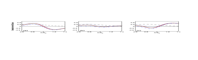
Figure 1: (color online, two column wide) This figure shows the result of different pricing formulas from which the Black-Scholes result (with interest rate $r=\theta_{r}$) has been subtracted. Since we are not considering a specific asset, the option price could be stated in any currency, therefore the deviation is given in arbitrary units. The thick (red) curve shows our analytical results for the model with both stochastic interest rate $r$ and stochastic volatility. The crosses represent results from a Monte Carlo simulation of our model, confirming the analytical formula. The blue dotted curve and the blue dash-dotted curve show the results for the Heston model with constant interest rate $r=r(0)$ and $r=\theta_{r}$, respectively. The dashed curve shows the results for a Black-Scholes model with $r=r(0).$ The following parameter values were used for all three panels: $\kappa=1$, $\sigma=0.2$, $\theta=0.04$, $v_{0}=0.04$, $T=1$, $S_{0}=100$, $\kappa_{r}=1.8$; $\sigma_{r}=0.1$; $\theta_{r}=0.03$; $r_{0}=0.035$. The correlation coefficient is for panel (a) $\rho=-0.5,$ (b) $\rho=0$ and (c) $\rho=0.5$.

This is illustrated in Fig. 1, where the different approaches are compared. Let’s start with the most complete model, where both interest rate and volatility are stochastic. The resulting option price, Eq. (41), for this model is shown as a thick red curve. The result from the closed-form expression agrees well with the Monte Carlo simulation, shown as crosses.

Now we strip off one layer of complexity, and fix the interest rate $r$ – it is no longer a stochastic variable. Then we obtain the Heston model as an ‘approximation’ to a stochastic interest rate world. The question poses itself of which fixed interest rate to use, if we want to make the comparison. Two choices are shown in Fig. 1: $r=r(0)$ and $r=\theta_{r}$. The former choice (dotted blue curves) sets the Heston interest rate equal to the interest rate at time $0$, whereas the latter choice (dash-dotted curves) sets the Heston interest rate equal to the mean reversion level $\theta_{r}$. For the parameter values used in Fig. 1, the most complete result lies between the two Heston ‘approximations’, but this is not necessarily so. Fig. 2 shows that for some choices of other (realistic) parameters, the full result can lie outside both Heston approximations. Nevertheless, as $\kappa$ becomes very large, the stochastic interest rate will be drawn very tightly to the mean reversion rate $\theta_{r}$, and one expects the full result to be near the Heston approximation with $r=\theta_{r}$. When $\kappa$ is very small, the stochastic interest rate will not be drawn quickly towards $\theta_{r}$ so that when also $\sigma_{r}$ is small, the full results will be near the Heston approximation with $r=r(0)$.

Next, we strip off the second layer of approximation, and also fix the volatility. This results in the familiar Black-Scholes model as the crudest approximation to our system. Now a second choice has to be made: which value of the volatility to use. Here, we take the stochastic volatility at time zero to be equal to the mean reversion level of the volatility CIR process, so that the ambiguity of choice is avoided. The choice for what interest rate to use, however, remains. In Fig. 1, we show the Black-Scholes results with $r=r(0)$ (dashed line) and $r=\theta_{r}$ (full line). We have plotted all the results relative to the Black-Scholes result with $r=\theta_{r}$ to emphasize the differences rather than the absolute magnitude of the prices (for this reason, the $r=\theta_{r}$ Black-Scholes result is the baseline of the plots). The difference between the three panels of Fig. 1 is the value of the correlation between asset price and volatility.

Figure 2: (color online). As in Fig. 1, the result of different pricing formulas from which the Black-Scholes result (with interest rate $r=\theta_{r}$, thin black line) has been subtracted, is shown. The following parameter values were used: $\kappa=1$, $\sigma=0.2$, $\theta=0.04$, $v_{0}=0.04$, $T=1$, $S_{0}=100$, $\kappa_{r}=0.5$, $\sigma_{r}=0.3$, $\theta_{r}=0.03$, $r_{0}=0.035$, $\rho=0$.

From Figs. 1 and 2, it is clear that both levels of approximation (keeping the volatility constant and keeping the interest rate constant) have an equally large effect on the option price. Even within the Heston framework, the choice of what value to use for the interest rate is seen to influence the price considerably. Choosing a different interest rate, or keeping the interest rate as a stochastic variable, leads to a price correction that is as large as the price correction obtained by going from the Black-Scholes to the Heston model. This result emphasizes the importance of a correct treatment of the interest rate in pricing models (This also depends strongly on the length of the lifetime of the option).

Finally we must remark that the price differences when working within the standard Heston model or within the extended one can be influenced by the calibration method. For Figures. 1 and 2 we used the same parameters for the volatility process both in the standard model and in the extended one, parameter values for the interest rate process are calibrated separately. Literature shows that the parameter values for the volatility process (see for example jap2 and Heston ) and the interest rate process (see for example Dsev and Brown ) can attain values in a broad range containing the values we chose to produce Fig. 1 and Fig. 2. However if the parameter values obtained for the interest rate process are used in formula (41) to calibrate the remaining parameter values for the volatility process one might get different results. We can not exclude that this calibration approach would lead to smaller price differences between the two approaches. However such a calibration is a research area on its own and is outside the scope of this article.

IV Conclusions

We have developed a path-integral method to derive closed-form analytical formulas for the asset price distribution in the Heston stochastic volatility model. Closed-form formulas are obtained for the logreturn of the derivative and the vanilla option price. The presented results correspond to the known semi-analytic results obtained from solving the partial differential equation Heston by standard techniques.

The flexibility of our approach is demonstrated by extending the results to the case where the interest rate is a stochastic variable as well, and follows a CIR process. For this case, to the best of our knowledge, no exact analytical solutions have been derived before. We have checked our semi-analytical results for the model with both stochastic volatility and stochastic interest rate against a Monte-Carlo simulation. The quantitative analysis shows that the effect of stochastic interest rate on the Heston model can be as large as the effect of the stochastic volatility on the Black-Scholes model. However we did not perform a full calibration, which might influence the results. Finally, the analogy between stochastic interest rate models and path dependent options makes our method promising for the pricing of exotic derivative products.

- (1) F. Black and M. Scholes, J. Pol. Econ. 81 637 (1973).
- (2) R. C. Merton, Bell Journal of Economics and Management Science, 4, 141 (1973)
- (3) B. E. Baaquie, Quantum Finance: Path Integrals and Hamiltonians for Options and Interest Rates (Cambridge University Press, Cambridge, 2004).
- (4) H. Kleinert, Path Integrals in Quantum Mechanics, Statistics, Polymer Physics, and Financial Markets, (World Scientific, Singapore, 2004).
- (5) J. Dash, Quantitative Finance and Risk Management: A Physicist’s Approach.
- (6) P. Wilmott, J. Dewynne, and S. Howison, Option Pricing (Oxford Financial Press, Oxford, 1993).
- (7) R. Cont, P. Tankov, Financial modelling with jump processes, Chapman & Hall/CRC, (2003).
- (8) E. Derman, I. Kani, Riding on a smile, Risk 7 (1994) 32-39.
- (9) W. Schoutens, Levy Processes in Finance: Pricing Financial derivatives, Wiley, 2003.
- (10) A. Lipton, Mathematical Methods for Foreign Exchange: A Financial Engineer’s Approach, World Scientific, 2001.
- (11) S. L. Heston, Review of Financial Studies 6, 327 (1993).
- (12) P. Cizek, W. Härdle and R. Weron, Statistical Tools for Finance and Insurance, Springer, 2005.
- (13) S. Griebsch, Pricing of Exotic options in Heston’s stochastic volatility model, Lecture, Frankfurt Mathfinance Workshop, March 2007.
- (14) L. B. G. Andersen, ”Efficient Simulation of the Heston Stochastic Volatility Model” (January 23, 2007). Available at SSRN: http://ssrn.com/abstract=946405.
- (15) V. Linetsky, Computational Economics 11, 129 (1998).
- (16) J. Dash, Path integrals and options: Part I. (CNRS preprint CPT-88/PE.2206, 1988).
- (17) J. Dash, Path integrals and options: Part II. (CNRS preprint CPT-89/PE.2333, 1989).
- (18) A. A. Drăgulescu, arXiv:cond-mat/0307341.
- (19) B. E. Baaquie, J. Phys. I France 7, 1733 (1997).
- (20) H. Kleinert, Physica A 338, 151 (2004).
- (21) E. M. Stein and J. C. Stein, Review of Financial Studies 4, 727 (1991).
- (22) A. A. Drăgulescu and V. M. Yakovenko Quantitative Finance 2 443-453 (2002).
- (23) A. C. Silva and V. M. Yakovenko Physica A 324 303 – 310 (2003).
- (24) J. E. Zhang and J. Shu, Proceedings of the IEEE International Conference on Computational Intelligence for Financial Engineering, 2003, pages 85-92.
- (25) Y. Aït-Sahalia and R. Kimmel Journal of Financial Economics volume 83 issue 2 pages 413-452 (2007).
- (26) G. Fiorentini, A. León and G. Rubio Journal of Empirical Finance volume 9 issue 2 pages 225-255 (2002).
- (27) S. R. Das and R. K. Sundaram, Journal of Financial and Quantitative Analysis volume 34 issue 2 pages 211-239 (1999).
- (28) R. Rebonato, Volatility and Correlation: the Perfect Hedger and the Fox, 2e Edition (John Wiley, Chichester, 2004).
- (29) J. P. Bouchaud and M. Potters Theory of Financial Risk and Derivative Pricing (Cambridge University Press, New York, 2003).
- (30) P. Gopikrishnan, V. Plerou, L. A. N. Amaral, M. Meyer and H. E. Stanley PRE 60, 5 (1999).
- (31) R. P. Feynman ; Statistical Mechanics: A Set of Lectures, Advanced Book Classics, 2e Edition (Perseus Books Group 1998).
- (32) J.C. Cox , J.E. Ingersoll, and S.A. Ross, Econometrica 53, 385 (1985).
- (33) R. H. Brown and S. M. Schaefer, Journal of Financial Economics, Volume 35, Issue 1, pages 3-42 (1994).
- (34) M. R. Gibbons and K. Ramaswamy, The Review of Financial Studies, Volume 6, Issue 3 pages 619-658 (1993).
- (35) D. Ševčovič and A. Urbánová Csajková, Cejor 13 169-188 (2005).
- (36) E. Bennati, M. Rosa-Clot, and S. Taddei, International Journal of Theoretical & Applied Finance 2, 381 (1999); also at arXiv:cond-mat/9901277.
- (37) C. Grosche and F.Steiner, Handbook of Feynman path integrals. (Springer, Berlin, 1998).
- (38) A. P. Prudnikov, Y. A. Brychkov, and O. I. Marichev Integrals and series, volume 2: special functions (Gordon and Breach, New York, 1992).
- (39) N. Kunitomo and Y. J. Kim, The Japanese Economic Review 58, 71 (2007).