X-ray time variability across the atoll source states of 4U 1636–53

Abstract

We have studied the rapid X-ray time variability in 149 pointed observations with the Rossi X-ray Timing Explorer (RXTE)’s Proportional Counter Array of the atoll source 4U 1636–53 in the banana state and, for the first time with RXTE, in the island state. We compare the frequencies of the variability components of 4U 1636–53 with those in other atoll and Z-sources and find that 4U 1636–53 follows the universal scheme of correlations previously found for other atoll sources at (sometimes much) lower luminosities. Our results on the hectohertz QPO suggest that the mechanism that sets its frequency differs from that for the other components, while the amplitude setting mechanism is common. A previously proposed interpretation of the narrow low-frequency QPO frequencies in different sources in terms of harmonic mode switching is not supported by our data, nor by some previous data on other sources and the frequency range that this QPO covers is found not to be related to spin, angular momentum or luminosity.

1. Introduction

Low-mass X-ray binaries (LMXBs) can be divided into systems containing a black hole candidate (BHC) and those containing a neutron star (NS). The accretion process onto these compact objects can be studied through the timing properties of the associated X-ray emission (see, e.g., van der Klis, 2006, for a review). Hasinger & van der Klis (1989) classified the NS LMXBs based on the correlated variations of the X-ray spectral and rapid X-ray variability properties. They distinguished two sub-types of NS LMXBs, the Z sources and the atoll sources, whose names were inspired by the shapes of the tracks that they trace out in an X-ray color-color diagram on time scales of hours to days. The Z sources are the most luminous; the atoll sources cover a much wider range in luminosities (e.g. , Ford et al., 2000, and references therein). For each type of source, several spectral/timing states are identified which are thought to arise from qualitatively different inner flow configurations. In the case of atoll sources, the main three states are the extreme island state (EIS), the island state (IS) and the banana branch, the latter subdivided into lower-left banana (LLB), lower banana (LB) and upper banana (UB) states. Each state is characterized by a unique combination of color color diagram and timing behavior. The EIS and the IS occupy the spectrally harder parts of the color color diagram (CD) corresponding to lower X-ray luminosity ($L_{x}$). The different patterns they show in the CD are traced out in days to weeks. The hardest and lowest $L_{x}$ state is generally the EIS, which shows strong low-frequency flat-topped noise. The IS is spectrally softer than the EIS. Its power spectrum is characterized by broad features and a dominant band-limited noise (BLN) component which becomes stronger and lower in characteristic frequency as the flux decreases and the $>6$ keV spectrum gets harder. In order of increasing $L_{x}$ we encounter the LLB, where the twin kHz QPOs are first observed, the LB, where dominant 10-Hz BLN occurs and finally, the UB, where the $<1$ Hz (power law) very low frequency noise (VLFN) dominates. In the banana states, some of the broad features observed in the EIS and the IS become narrower (peaked) and occur at higher frequency. The twin kHz QPOs can be found in LLB at frequencies in excess of 1000 Hz, only one is seen in the LB, and no kHz QPOs are detected in the UB (see reviews by Hasinger & van der Klis, 1989; van der Klis, 2000, 2004, 2006, for detailed descriptions of the different states).

4U 1636–53 is an atoll source (Hasinger & van der Klis, 1989) which has an orbital period of $\sim 3.8$ hours (van Paradijs et al., 1990) and a companion star with a mass of $\sim 0.4\ M_{\odot}$ (assuming a NS of $\sim 1.4\ M_{\odot}$, see Giles et al., 2002, for a discussion). It was first observed as a strong continuous X-ray source (Norma X-1) with Copernicus (Willmore et al., 1974) and Uhuru (Giacconi et al., 1974). 4U 1636–53 is an X-ray burst source (Hoffman et al., 1977) which shows asymptotic burst oscillation frequencies of $\sim 581$ Hz (see e.g. Zhang et al., 1997; Giles et al., 2002). This is probably the approximate spin frequency; although Miller (1999) presented evidence that these oscillations might actually be the second harmonic of a neutron star spin frequency of $\sim 290$ Hz, this was not confirmed in further work by Strohmayer (2001a). Prins & van der Klis (1997) studied the aperiodic timing behavior of 4U 1636–53 with the EXOSAT Medium Energy instrument up to frequencies of $\sim 100$ Hz both in the island and the banana state. Wijnands et al. (1997), using observations with RXTE, discovered two simultaneous quasi-periodic oscillations (QPOs) near 900 Hz and 1176 Hz when the source was in the banana state. The frequency difference $\Delta\nu$ between the two kHz QPO peaks is nearly equal to half the burst oscillation frequency, similar to what has been observed in other sources with burst oscillations or pulsation frequency $>400$ Hz. To the extent that this implies $\Delta\nu\sim\nu_{spin}/2$, this is inconsistent with spin-orbit beat-frequency models (Wijnands et al., 2003) for the kHz QPOs such as proposed by Miller et al. (1998). Other complications for beat frequency models include the fact that $\Delta\nu$ is neither constant (e.g. in Sco X-1, van der Klis et al., 1997) nor exactly equal to half the burst oscillation frequency. Generally, $\Delta\nu$ decreases as the kHz QPO frequency increases, and in 4U 1636–53, observations have shown $\Delta\nu$ at frequencies lower as well as higher than half the burst oscillation frequency (Mendez et al., 1998a; Jonker et al., 2002a).

van Straaten et al. (2002, 2003) compared the timing properties of 4U 0614+09, 4U 1608–52 and 4U 1728–34 and conclude that the frequencies of the variability components in these sources follow the same pattern of correlations. Di Salvo et al. (2003), based on five detections of kHz QPOs in 4U 1636–53 in the banana state was able to show that at least in that state the source might fit in with that same scheme of correlations. The detailed investigation of 4U 1636–53 is important because it is one of the most luminous atoll sources (Ford et al., 2000) that shows the full complement of island (this paper) and banana states and that also shares other timing features with often less luminous atoll sources. For example, Revnivtsev et al. (2001) found a new class of low frequency QPOs in the mHz range which they suggested to be associated with nuclear burning in 4U 1636–53 and 4U 1608–52. Méndez (2000) and Méndez et al. (2001) compared the relations between kHz QPOs and inferred mass accretion rate in 4U 1728–34, 4U 1608–52, Aql X-1 and 4U 1636–53, and showed that the dependence of the frequency of one of the kHz QPOs upon X-ray intensity is complex, but similar among sources. Jonker et al. (2000a) discovered a third kHz QPO in 4U 1608–52, 4U 1728–34, and 4U 1636–53 which is likely an upper sideband to the lower kHz QPO. Recently, Jonker et al. (2005) found in 4U 1636–53 an additional (fourth) kHz QPO, likely the corresponding lower sideband.

In this paper, we present new results for low frequency noise with characteristic frequencies $1-100$ Hz and QPOs in the range $100-1260$ Hz, for the first time including RXTE observations of the island state of this source. These results better constrain the timing behavior in the various states of 4U 1636–53. We compare our results mainly with those of the atoll sources 4U 0614+09, 4U 1608–52 and 4U 1728–34 and find that the frequency of the hectohertz component may not be constant as previously stated, but may have a sinusoidal like modulation within its range from $\sim 100$ to $\sim 250$ Hz. Our results also suggest that the mechanism that sets the frequency of the hHz QPOs differs from that for the other components, while the amplitude setting mechanism is common. Finally, we demonstrate that it is not possible to clearly distinguish between two harmonics of the low-frequency QPO $L_{LF}$ across different sources, as was previously thought (van Straaten et al., 2003).

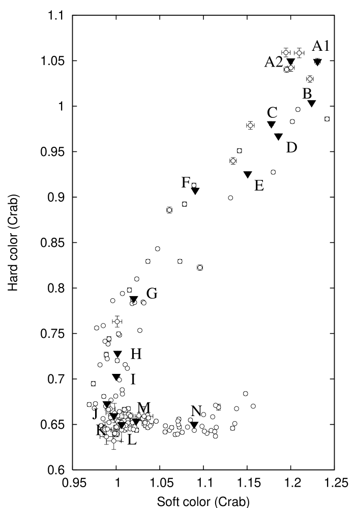
Figure 1.— Hard color versus soft color normalized to the Crab Nebula as explained in Section 1. Each circle represents the average soft/hard color of one of the observations used for this paper. The filled triangles mark averages of 1 to 32 observations and are labeled with letters, in order from ($A$) the island state, Lower Left Banana ($J$) to the Lower banana ($N$).

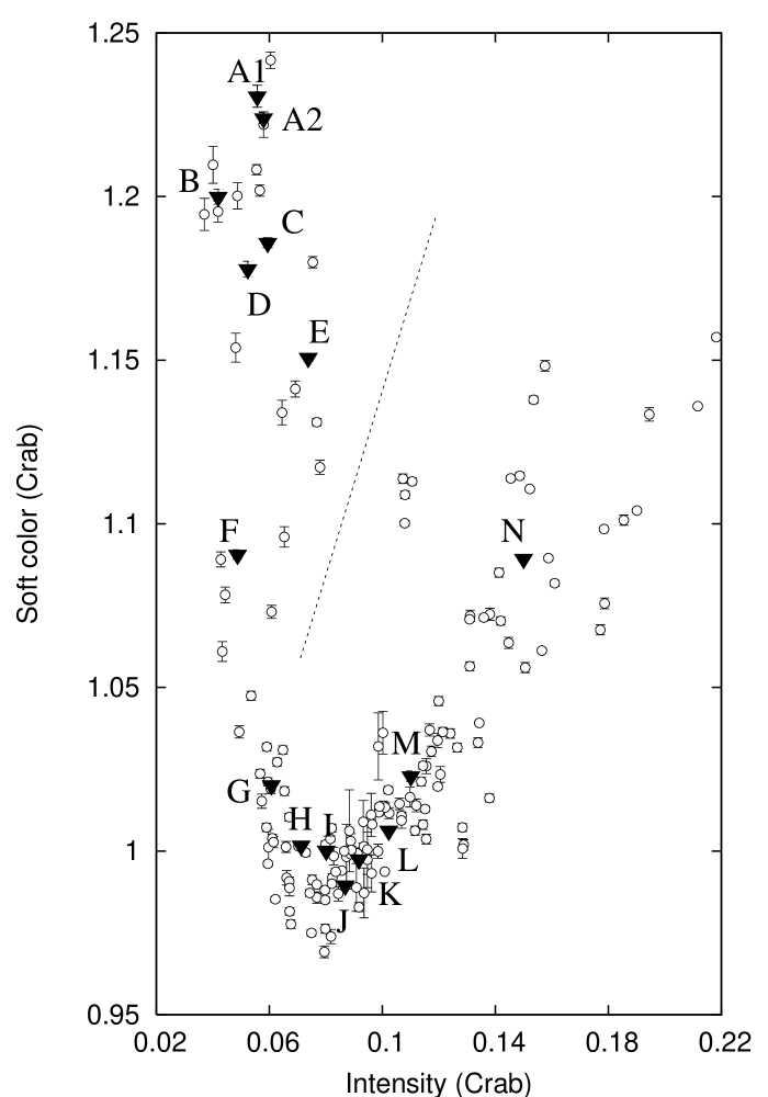
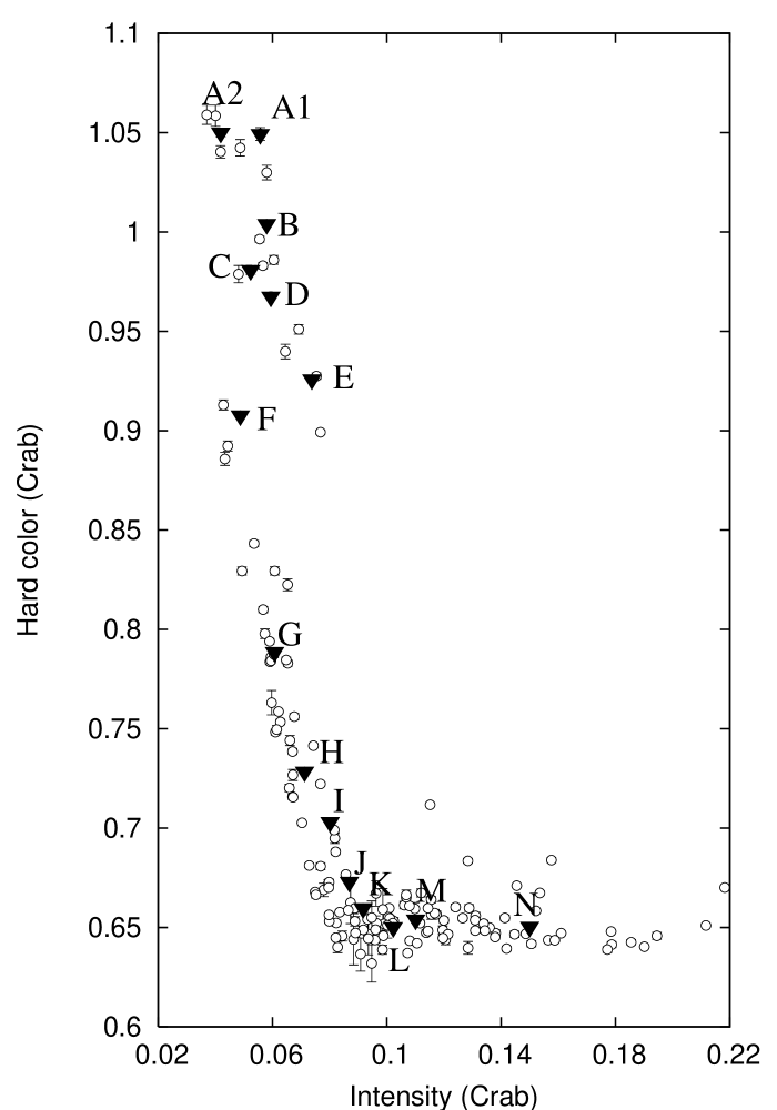
Figure 2.— Soft color vs. intensity (left) and hard color vs. intensity (right) in units of the Crab Nebula as explained in Section 1. Symbols as in Figure 1. For clarity, the dashed line separates the observations corresponding to the IS (left), from the observations corresponding to the BS (right).

2. OBSERVATIONS AND DATA ANALYSIS

We use data from the Rossi X-ray Timing Explorer (RXTE) Proportional Counter Array (PCA; for instrument information see Zhang et al., 1993). There were 149 pointed observations in the four data sets we used (60032-01, 60032-05, 70036-01, 80425-01 & 90409-01), each consisting of a fraction of one to several entire satellite orbits, for $\sim 1$ to $\sim 26$ ksec of useful data per observation. We use the 16-s time-resolution Standard 2 mode data to calculate X-ray colors as described in Altamirano et al. (2005). Hard and soft color are defined as the 9.7–16.0 keV / 6.0–9.7 keV and 3.5–6.0 keV / 2.0–3.5 keV count rate ratio, respectively, and intensity as the 2.0–16.0 keV count rate. Type I X-ray bursts were removed, background was subtracted and deadtime corrections were made. In order to correct for the gain changes as well as the differences in effective area between the PCUs themselves, we normalize our colors by the corresponding Crab color values (see Kuulkers et al., 1994; van Straaten et al., 2003) that are closest in time but in the same RXTE gain epoch, i.e., with the same high voltage setting of the PCUs (Jahoda et al., 2005). In Table 2 we show for reference the all-epoch averaged colors for Crab Nebula. All active PCUs were used to calculate the colors in 4U 1636–53 except for observation 60032-01-01-02, where due to a PCU3 malfunction we only used PCUs 0 and 2. Figure 1 shows the color-color diagram of the 149 different observations that we used for this analysis, and Figure 2 the corresponding hardness-intensity diagrams (soft and hard color vs. intensity).

For the Fourier timing analysis we used data from the $\sim 125\mu$s (1/8192 s) time resolution Event mode E_125us_64M_0_1s. First, we used a 2 second-binned light curve in order to detect and remove data drop-outs and X-ray bursts (these data were also excluded from the rest of the analysis). Leahy-normalized power spectra were constructed using data segments of 128 seconds and 1/8192s time bins such that the lowest available frequency is $1/128\approx 8\times 10^{-3}$ Hz and the Nyquist frequency 4096 Hz. No background or deadtime corrections were made prior to the calculation of the power spectra. We first averaged the power spectra per observation. We inspected the shape of the average power spectra at high frequency ( $>2000$ Hz) for unusual features in addition to the usual Poisson noise. None were found. We then subtracted a Poisson noise spectrum estimated from the power between 3000 and 4000 Hz, where neither intrinsic noise nor QPOs are known to be present, using the method developed by Klein-Wolt (2004) based on the analytical function of Zhang et al. (1995). The resulting power spectra were converted to squared fractional rms (van der Klis, 1995). In this normalization the square root of the integrated power density equals the variance of the intrinsic variability in the source count rate. In order to improve the statistics, observations were averaged together if they described the same source state. Since it is known from previous work on similar sources that the position of the source in the color-color diagram generally is well correlated to its spectral/timing state (see e.g. van der Klis, 2006, and references within), we first grouped observations with similar colors. Within each group, we then compared the shape of each average power spectrum with all of the other ones to create subgroups in which all power spectra had a dependence of power on frequency that was identical within errors. So, narrow features had to be at the same frequency for average power spectra to be added together. The resulting data selections are labeled interval A to N (see Table 1 for details on which observations were used for each interval and their colors). A disadvantage of this method is that we can loose information about narrow features moving on time scales shorter than an observation, such as the lower kilohertz QPO (see e.g. Berger et al., 1996; Di Salvo et al., 2003). The “shift and add” method (Mendez et al., 1998b), to some extent might be able to compensate for this; we explore in the Appendix this issue. Our method is the best suited one to study the behavior of the broad features such as typically seen in low mass X-ray binaries’ power spectra (e.g. van Straaten et al., 2002, 2003, 2005; Altamirano et al., 2005; Linares et al., 2005). For these broad components, which are the main aim of this paper, the gain in signal to noise due to this averaging process outweighs a minor additional broadening due to frequency variations.

Interval A1
Observation	Soft color (Crab)	Hard color (Crab)	Intensity (Crab)
80425-01-04-01	$1.2306\pm 0.0034$	$1.0493\pm 0.0032$	$0.0557\pm 0.0001$
Interval A2
80425-01-03-00	$1.2097\pm 0.0056$	$1.0585\pm 0.0053$	$0.0400\pm 0.0001$
90409-01-01-00	$1.1945\pm 0.0049$	$1.0590\pm 0.0049$	$0.0370\pm 0.0001$
90409-01-01-01	$1.1954\pm 0.0032$	$1.0403\pm 0.0031$	$0.0418\pm 0.0001$
90409-01-02-00	$1.2002\pm 0.0040$	$1.0424\pm 0.0042$	$0.0487\pm 0.0001$

Table 1Observations used for the timing analysis. The colors and intensity are normalized to Crab (See Section 2). The complete table can be obtained digitally from ApJ.

PCU Number	Crab’s soft color	Crab’s hard color	Crab’s intensity (c/s)
0	$2.21\pm 0.04$	$0.56\pm 0.009$	$2552\pm 21$
1	$2.27\pm 0.03$	$0.55\pm 0.008$	$2438\pm 21$
2	$2.22\pm 0.04$	$0.58\pm 0.010$	$2424\pm 20$
3	$2.42\pm 0.03$	$0.57\pm 0.009$	$2365\pm 20$
4	$2.34\pm 0.03$	$0.58\pm 0.011$	$2299\pm 21$

Table 2Average soft, hard and intensity of the Crab Nebula over all epochs and per PCU. Note that we have used averaged values per day in our analysis; the numbers listed here are representative for those daily averages. We quoted the averaged quadratic errors, i.e. $\sqrt{\sum_{i}^{n}\Delta\kappa^{2}_{i}}/n$, where $\Delta\kappa$ is either the soft, hard or the intensity day error.

To fit the power spectra, we used a multi-Lorentzian function: the sum of several Lorentzian components plus, if necessary, a power law to fit the very low frequency noise at $\lesssim 1$ Hz. Each Lorentzian component is denoted as $L_{i}$, where $i$ determines the type of component. The characteristic frequency ($\nu_{max}$ as defined below) of $L_{i}$ is denoted $\nu_{i}$. For example, $L_{u}$ identifies the upper kHz QPO and $\nu_{u}$ its characteristic frequency. By analogy, other components have names such as $L_{\ell}$ (lower kHz), $L_{hHz}$ (hectohertz), $L_{h}$ (hump), $L_{b}$ (break frequency), and their frequencies are $\nu_{\ell}$, $\nu_{hHz}$, $\nu_{h}$ and $\nu_{b}$, respectively. For reference, in Figure 3 we show two representative power spectra in which we labeled the different components. Using this multi-Lorentzian function makes it straightforward to directly compare the different components in 4U 1636–53 to those in previous works which used the same fit function (e.g., Belloni et al., 2002; van Straaten et al., 2002, 2003, 2005; Altamirano et al., 2005, and references therein).

Figure 3.— Representative power spectra of the island state (above - interval B) and the banana state (below - interval J) with their components.

We only include those Lorentzians in the fits whose single trial significance exceeds $3\sigma$ based on the negative error bar in the power integrated from 0 to $\infty$ (i.e. we include only those Lorentzians whose integral power is at least 3 times higher than zero based on the negative 1$\sigma$ error) and whose inclusion gives a $>3\sigma$ improvement of the fit according to an F-test. We give the frequency of the Lorentzians in terms of characteristic frequency $\nu_{max}$ as introduced by Belloni et al. (2002): $\nu_{max}=\sqrt{\nu^{2}_{0}+(FWHM/2)^{2}}=\nu_{0}\sqrt{1+1/4Q^{2}}$. For the quality factor $Q$ we use the standard definition $Q=\nu_{0}/FWHM$. FWHM is the full width at half maximum and $\nu_{0}$ the centroid frequency of the Lorentzian. Note that Q values in excess of $\sim 3$ will generally be affected by smearing in an analysis such as ours. Such values are commonly seen in $L_{LF}$, $L_{\ell}$ and $L_{u}$. In Section 3 we indicate in which cases this could have occurred.

We only report the results for $\nu_{max}\gtrsim 1$ Hz. 4U 1636–53 is one of three atoll sources which are known to show milihertz QPOs which affect the power law behavior of the noise at $\lesssim 1$ Hz (Revnivtsev et al., 2001). A different kind of analysis is needed to study these QPOs; we will report the results in a separate paper (Altamirano et al., 2008).

Interval	$\nu_{u0}$	$FWHM_{\nu_{u0}}^{*}$	$\nu_{\ell 0}$	$FWHM_{\nu_{\ell 0}}^{*}$	$\Delta\nu_{0}$	Ratio $\nu_{u0}/\nu_{\ell 0}$
H	$860.4\pm 1.7$	$136.2\pm 4.8$	$565.4\pm 5.1$	$90.4\pm 12.3$	$295.0\pm 5.4$	$1.52\pm 0.01$
I	$896.8\pm 2.6$	$115.8\pm 6.3$	$580.4\pm 5.1$	$77.2\pm 12.5$	$316.4\pm 5.7$	$1.54\pm 0.01$
J	$972.1\pm 3.5$	$98.0\pm 8.7$	$661.1\pm 1.8$	$73.8\pm 4.1$	$311.0\pm 3.9$	$1.470\pm 0.006$
K	$992.9\pm 6.6$	$177.4\pm 16.9$	$718.3\pm 2.4$	$121.5\pm 6.3$	$274.6\pm 5.7$	$1.38\pm 0.01$
L	$1147.2\pm 16.6$	$123.4\pm 27.8$	$836.1\pm 0.7$	$64.1\pm 1.9$	$311.1\pm 16.6$	$1.37\pm 0.02$

Table 3Central frequencies, full width at half maximum (FWHM) and the frequency difference $\Delta\nu_{0}$ between the kHz QPOs for the 5 intervals where both kHz QPOs where detected significantly ($>3\sigma$). ^∗: Note that these values might have been affected by smearing (see text) .

3. Results

Figures 1 and 2 show that in order A to H, the spectrum becomes softer (i.e. hard and soft color both decrease), and the intensity changes little. From H to L the soft color remains approximately constant but above 6 keV the spectrum becomes even steeper (i.e., the hard color decreases further) and, from interval G, the intensity increases. Finally from L to N, below 6 keV the spectrum becomes flatter and above 6 keV it remains approximately constant in slope, while the intensity continues increasing. Similar behavior has been observed in other atoll sources which are moving from the island to the lower left banana and then to the lower banana state (see for example van Straaten et al., 2003; Altamirano et al., 2005).

In Figure 4 we show the average power spectra $A-N$ with their fits. Two to five Lorentzian components were needed for a good fit, except in power spectrum I, where an extra component is needed, for a total of six. Table LABEL:table:data gives the fit results. Power spectra A1 and A2 have the same $\nu_{u}$ within errors, and only slightly different colors. We treat these two power spectra separately because A1 could be fitted with 5 significant components and A2, as well as the combined spectrum A1+A2, only with 3. Note, that power spectrum A1 is the average of one observation (See Table 1) which was performed in between the observations used for power spectrum A2. In Figure 5 we show our measured characteristic frequency correlations (black) together with those previously measured in other atoll sources (grey). In intervals H–L, the twin kilohertz QPOs ($L_{u}$ and $L_{\ell}$) are identified unambiguously. The correlation between the lower and the upper kilohertz QPO is the same as that found in the other atoll sources studied by van Straaten et al. (2003). For intervals M and N, only $L_{u}$ is observed.

Figure 4.— Power spectra and fit functions in the power spectral density times frequency representation. Each plot corresponds to a different region in the color-color and color-intensity diagrams (See Figures 1 and 2). The curves mark the individual Lorentzian components of the fit. For a detailed identification, see Table LABEL:table:data and Figure 5.

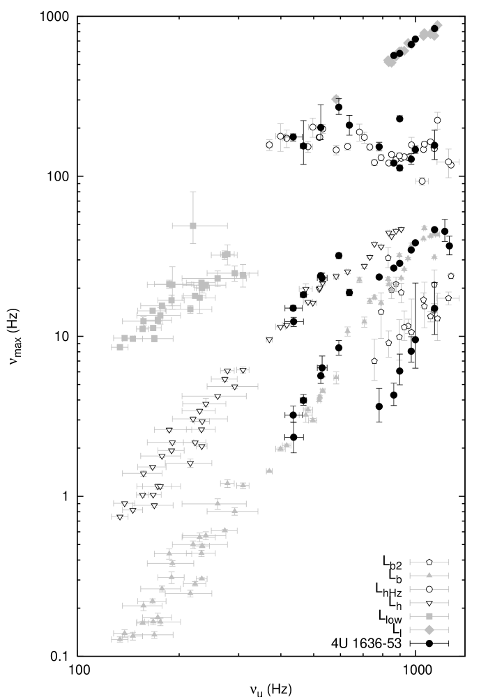
Figure 5.— The characteristic frequencies $\nu_{max}$ of the various power spectral components plotted versus $\nu_{u}$. The black bullets mark the results for 4U 1636–53. The other symbols mark the atoll sources 4U 0614+09, 4U 1728–34 (van Straaten et al., 2002), 4U 1608–52 (van Straaten et al., 2003), and Aql X-1 (Reig et al., 2004) and the low luminosity bursters 1E 1724–3045, GS 1826–24 and SLX 1735–269 (van Straaten et al., 2005, but also see Belloni et al. 2002).

We separately measured the centroid frequencies $\nu_{0}$ of the kHz QPOs (see Table 3). The centroid frequency difference $\Delta\nu$ varied between $274.6\pm 5.7$ Hz (in interval K) and $316.4\pm 5.7$ Hz (interval I). These values are between the extremes found by Jonker et al. (2002a) ($\Delta\nu=330\pm 9$ Hz) and Di Salvo et al. (2003) ($\Delta\nu=242\pm 4$ Hz). Note that those authors used much shorter time intervals to detect the kHz QPOs and hence were more sensitive to short lived extreme cases. Our average power spectra contain those data which is necessary to detect the broad components well, and hence our measured $\Delta\nu$’s occur at intermediate values, which is when the kHz QPOs are strongest (see e.g. Méndez et al., 2001). So our method averages out the extreme cases. In power spectrum N, $L_{u}$ reaches the highest centroid frequency found among the intervals analyzed, $1259\pm 10$ Hz. Note that power spectra M and N are the result of averaging large amounts of data with no significant kHz QPOs in individual observations ($\sim 2.2\times 10^{4}$ seconds and $\sim 2.5\times 10^{5}$ seconds, respectively), based on the position of 4U 1636–53 in the color-color diagram. Figure 6 displays the upper kHz QPOs in power spectra M and N more clearly.

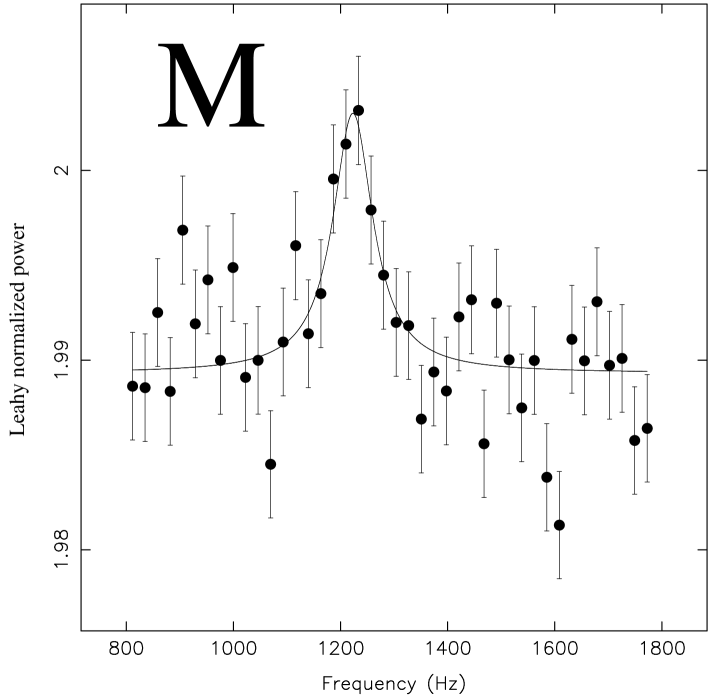
Figure 6.— kHz QPOs of intervals $M$ and $N$, respectively. These are Leahy normalized power spectra with no Poisson noise subtraction.

Between $\sim 100$ Hz and $\sim 200$ Hz, a Lorentzian with quality factor $Q\sim 1$ is often found in atoll sources (see van der Klis, 2004, and references therein). This feature is called hectohertz QPO and, in contrast to the other components, its frequency remains confined to this relatively narrow range as $\nu_{u}$ increases. When $\nu_{u}\gtrsim 800$ Hz, the twin kilohertz QPOs are usually identified unambiguously, and so is the hectohertz QPO. For $\nu_{u}\lesssim 600$ Hz, the lower kHz QPO could also have frequencies between $\sim 100$ Hz and $\sim 300$ Hz if it would be present, which makes it difficult to classify the QPOs found in that range as either $L_{\ell}$, $L_{hHz}$ or a blend without more information. In our data, this is the case for intervals A to E; in Table LABEL:table:data and hereafter we identify those Lorentzians as hectohertz QPOs. This identification is supported by the fact that in intervals F and G, i.e., for 600 $<\nu_{u}<$ 800 Hz, $L_{\ell}$ is undetected; this component seems to appear only at $\nu_{u}>800$ Hz. Interval I shows a $\sim 3.1\sigma$ (single trial) peak with $\nu_{max}=229\pm 9$ Hz which is a factor $\sim$2 higher than the usual hHz in that range. This QPO may be the second harmonic of the hectohertz QPO simultaneously found at a characteristic frequency of $113\pm 4$ Hz (see Figure 7, however, note that this feature must be interpreted with care due to its low -3.1$\sigma$- single trial significance). As a result of refitting the power spectrum using centroid frequencies, we find that the second harmonic QPO is at $\nu_{0}=228\pm 10$ Hz while the first harmonic hHz QPO is at $\nu_{0}=107\pm 5$ Hz for a ratio of $2.13\pm 0.13$, consistent with 2.

Figure 5 shows that also $L_{h}$ and $L_{b}$ lie on the correlations previously observed in other sources. However, our results show that $\nu_{b}$ may anti-correlate with $\nu_{u}$ at $\nu_{u}\gtrsim 1100$ Hz. This result has already been observed in Z sources, however for atoll sources this behavior has not been observed with certainty (See Section 4). $L_{b2}$ seems to have lower frequencies than in other atoll sources. To further investigate this, in Figure 8 we plot $\nu_{b2}$ versus $\nu_{u}$ with different symbols for each of the 4 atoll sources for which this component has been measured. Clearly, the range in which $L_{b2}$ has been found for similar $\nu_{u}$ is rather large (up to nearly a decade), particularly at $\nu_{u}<1000$ Hz. We also studied the possibility that the rms of $L_{b2}$ could be related with its frequency, but no relation was found.

Figure 7.— Part of the power spectrum of interval I, showing the twin kHz QPOs, the hHz QPO and its possible harmonic. This is a Leahy normalized power spectrum with no Poisson noise subtraction.

Figure 8.— $\nu_{b2}$ versus $\nu_{u}$ for the 4 atoll sources 4U 0614+09, 4U 1728–34 (van Straaten et al., 2002), 4U 1608–52 (van Straaten et al., 2003) and 4U 1636–53 (this paper). Note that the open square at $\nu_{u}\sim 1233$ Hz could be interpreted as either $L_{b}$ or $L_{b2}$ (van Straaten et al., 2002).

Intervals A, B, D and E show a narrow QPO with a characteristic frequency between $\nu_{b}$ and $\nu_{h}$ (see Table LABEL:table:data). For other neutron stars such narrow QPOs were previously reported by Yoshida et al. (1993) in 4U 1608–52, by Belloni et al. (2002) in the low luminosity bursters 1E 1724–3045 and GS 1826–24, by van Straaten et al. (2002) in 4U 0614+09, 4U 1728–34, by van Straaten et al. (2003) in 4U 1608-52, by Altamirano et al. (2005) in 4U 1820–30, by van Straaten et al. (2005) in the accreting millisecond pulsars (AMP) XTE J0929–314, XTE J1814–338 and SAX J1808.4–3658 and by Linares et al. (2005) in XTE J1807–294. Similar features were also seen in the BHCs Cyg X-1 by Pottschmidt et al. (2003) and GX 339–4 by Belloni et al. (2002, but also see ). Following van Straaten et al. (2003), for clarity we have omitted these QPOs ($L_{LF}$) from Figure 5. In Figure 9 we plot their characteristic frequencies vs. $\nu_{h}$. The results for 4U 1636–53 are in the range of, but seem to follow a different relation than, the two relations previously suggested by van Straaten et al. (2003) based on other sources. The $L_{LF}$ QPOs in 4U 1636–53 cannot be significantly detected on timescales shorter than the duration of an average observation.

For completeness, in Figure 10 we plot both the fractional rms amplitude and quality factor of the $L_{LF}$ component versus $\nu_{u}$. Although the fractional rms amplitude of 4U 1636–53 increases with $\nu_{u}$, no general trend is observed among the 7 sources shown in this Figure. The quality factor $Q_{LF}$ (which may have been affected by smearing, see Section 2) seems to be unrelated to $\nu_{u}$ for all the sources shown.

In Figure 11 we plot the fractional rms amplitude of all components (except $L_{LF}$, see Figure 10) versus $\nu_{u}$ for the atoll sources 4U 0614+09, 4U 1728–34, 4U 1608–52 and 4U 1636–53. The rms of the upper kHz QPO for all sources approximately follows the same trend: it increases up to $\nu_{u}\sim 750-800$ Hz, and then starts to decrease. This seems also to be the case for $L_{hHz}$ and $L_{b}$. Except for 4U 0614+09, the data suggest that at $\nu_{u}\gtrsim 1100$ Hz the rms of $L_{u}$ does not decrease further, but remains approximately constant. At $\nu_{u}\sim 750-800$ Hz, the rms amplitudes of $L_{hHz}$ and $L_{b}$ start to decrease (see also van Straaten et al., 2003). The rms of $L_{h}$ of 4U 1636–53 also seems to follow the general trends observed for the other atoll sources. Some of these results were previously reported by van Straaten et al. (2003), Méndez et al. (2001) and Barret et al. (2005a). 4U 1636–53 stands out by the fact that the rms of $L_{b2}$ and $L_{hHz}$ at $\nu_{u}\lesssim 900$ Hz is always smaller than in the other sources. Moreover, and again contrary to the other sources, in 4U 1636–53 the rms of $L_{b2}$ remains approximately constant as $\nu_{u}$ increases from $\sim 800$ Hz to $\sim 1200$ Hz.

Figure 9.— (Above) Characteristic frequencies $\nu_{LF}$ and $\nu_{LF/2}$ (see text) versus $\nu_{h}$ . The symbols are labeled in the plot, and represent the frequencies of the QPOs in the atoll sources 4U 1728–34, 4U 0614+09, 4U 1608–52, 4U 1820–30, the BHCs Cyg X-1 and GX 339–4, the low luminosity bursters 1E 1724–3045 and GS 1826–24 and the accreting millisecond pulsars XTE J0929–314, XTE J1814–338 and SAX J1808.4–3658 (van Straaten et al., 2003, 2005; Altamirano et al., 2005). The filled triangles show the results for 4U 1636–53. The drawn line indicates a power-law fit to the $\nu_{LF}$ vs. $\nu_{h}$ relation of the low-luminosity bursters 1E 1724–3045 and GS 1826–24, and the BHC GX 339–4. The dashed line is a power law with a normalization half of that of the drawn line. (Bottom) A zoom of the high frequency region.

In Figure 12 we plot the quality factors $Q_{u}$, $Q_{\ell}$ and $Q_{hHz}$ versus $\nu_{u}$. As noted in Section 2, the Q values of $L_{\ell}$, and to a lesser extent, $L_{u}$, have likely been affected by smearing. The Q values of the other components are not plotted since they are usually broad. The data on 4U 1636–53 are in general agreement with what was found using similar methods on the other sources (van Straaten et al., 2002). $Q_{u}$ increases monotonically with $\nu_{u}$ until $\nu_{u}\sim 900-1000$ Hz. At this frequency, $Q_{u}$ seems to decrease for all sources, to immediately increase again as $\nu_{u}$ increases. $Q_{\ell}$ shows a rather random behavior due to smearing (see Di Salvo et al. 2003 and Barret et al. 2005a, b for $Q_{\ell}$ measurements less affected by smearing); we display this quantity in Figure 12 for comparison to previous works using the same method.

$Q_{hHz}$ shows a complicated behavior. To further investigate this behavior, we first re-binned the $Q_{hHz}$ data by a factor 3 and fitted a straight line. The best fit gives $\chi^{2}/dof=93/12\sim 7.7$. Since the data appears to show two bumps separated by a minimum creating a roughly sinusoidal pattern, we also tried to fit a straight line plus a sine wave. The best fit has a $\chi^{2}/dof=16.9/9\sim 1.8$ which gives a $3.4\sigma$ improvement of the fit based on an F-test. In Figure 5 it can be seen that $\nu_{hHz}$ appears to display a similar pattern. Fitting the relation of $\nu_{hHz}$ versus $\nu_{u}$ with only a straight line gives a $\chi^{2}/dof=156/12=13$ while a straight line plus a sine gives a $\chi^{2}/dof=28.4/9\sim 3.15$, once again, we find a $3.4\sigma$ improvement of the fit based on an F-test. The results of the sinusoidal fits, in which the parameter errors have been rescaled by the reduced $\sqrt{\chi^{2}}$ value, are given in Table 4.

With the present data it is difficult to distinguish if this is the behavior of $L_{hHz}$ alone, or is due to blending with other components which are not strong and coherent enough to be observed separately on short time scales and are lost in the averaging of the power spectra. This, as well as other ambiguities (see discussion about the identification of $L_{\ell ow}$ in van Straaten et al. 2003), arise because of the gaps between the $\nu_{\ell}$, $\nu_{\ell ow}$, $\nu_{h}$ and $\nu_{hHz}$ versus $\nu_{u}$ relations (See Figure 5). Although we are not able to explain those gaps, the interpretation that $L_{hHz}$ could be affected by the presence of other components is made more likely by the fact that $L_{\ell}$ in Z sources can be unambiguously identified down to frequencies of $\sim 150$ Hz (see e.g. Jonker et al. 2002b) and that $L_{h}$ and $L_{\ell ow}$ have sometimes been observed at frequencies up to $\sim 120$ and $\sim 60$ Hz, respectively, i.e., in both cases reaching the hectohertz QPO range (van Straaten et al. 2005, Linares et al. 2005). If it would be possible to follow a source in its evolution from the extreme island states where $L_{\ell ow}$ is prominent, to the lower left banana where $L_{\ell}$ is seen, then some of these ambiguities could be resolved.

	$Q_{hHz}$	$\nu_{hHz}(Hz)$
Slope	$(1.6\pm 0.2)\cdot 10^{-3}$	$(-5.7\pm 1.1)\cdot 10^{-2}$
Constant	$-0.52\pm 0.15$	$196\pm 10$
Amplitude	$0.35\pm 0.04$	$23.5\pm 2.1$
Period	$532\pm 48$	$498\pm 25$
$\chi^{2}/dof$	15.1 / 15	14.9 / 15

Table 4The results of fitting the data of $Q_{hHz}$ and $\nu_{hHz}$ versus that of $\nu_{u}$ for the four atoll sources 4U 1728–34, 4U 0614+09, 4U 1608–52 and 4U 1636–53. We used the combination of a straight line plus a sine. The parameter errors have been rescaled by the reduced $\sqrt{\chi^{2}}$ value (see text). The quoted errors use $\Delta\chi^{2}=1.0$.

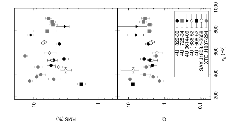
Figure 10.— $L_{LF}$’s rms (above) and Q (below) versus $\nu_{u}$ for 7 atoll sources. The symbols are labeled are the same in both plots. The scatter of the points are likely due to the averaging method (see text).

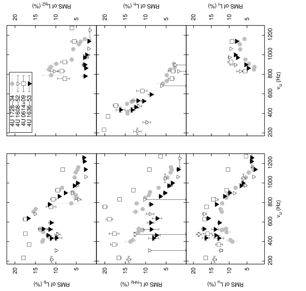
Figure 11.— The fractional rms amplitude of all components (except $L_{LF}$) plotted versus $\nu_{u}$. The symbols are labeled in the plot. The data for 4U 1728–34, 4U 1608–52 and 4U 0614+09 were taken from van Straaten et al. (2005). Note that for $L_{hHz}$ and $L_{h}$ of 4U 1608–52, the 3 triangles with vertical error bars which intersect the abscissa represent 95% confidence upper limits (see van Straaten et al. (2003) for a discussion). Also note that we exclude the 3 points in the $rms_{\ell}$ versus $\nu_{u}$ plot which were identified as $L_{low}$ by van Straaten et al. (2003).

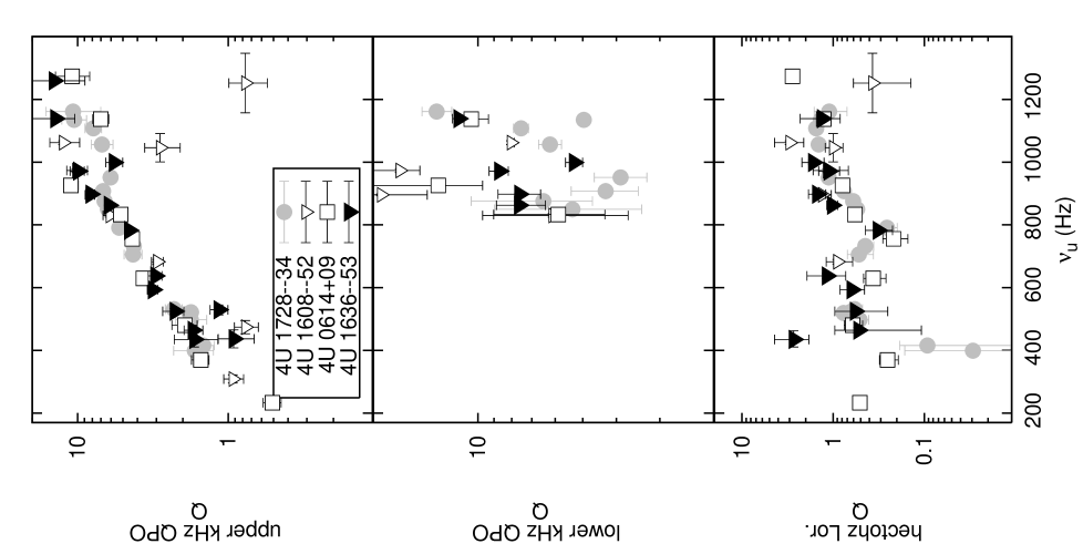
Figure 12.— Quality factor Q of $L_{u}$, $L_{\ell}$ and $L_{hHz}$ versus $\nu_{u}$. Symbols are the same as in Figure 11. Note that the results for the quality factor are probably affected by the averaging method (See Sections 1, 3 and the Appendix).

4. Discussion

In this paper, we report a detailed study of the time variability of the atoll source 4U 1636–53 using RXTE that includes, for the first time, observations of this source in the (low-luminosity) island state. We divided the data into 15 intervals, A to N, based on the position of the source in the color diagram. Based on the fact that, (i) intervals A1, B, D and E show a narrow QPO with a characteristic frequency between $\nu_{b}$ and $\nu_{h}$ which was previously seen in other atoll sources when they were in their island state (e.g. van Straaten et al., 2002; Altamirano et al., 2005); (ii) intervals A1, A2, B, D, E and F do not show either $L_{\ell}$ or power-law VLFN at frequencies lower than $0.5$ Hz, which would be expected to be present in the banana state (Hasinger & van der Klis, 1989; van der Klis, 2004, 2006); (iii) the intensity of the source starts to increase from interval G (see Figure 2) and (iv) intervals A1 to F occupy the hardest loci in the color diagram (see Figures 5 and 2), we conclude that intervals A1 to F show the source in the island state, representing the first RXTE observations of 4U 1636–53 in this state. Interval G may represent the transition between the IS and the LLB since its power spectrum is very similar to that of the first five intervals, but with the difference that a weak ($\sim 1.2~{}\%$ rms) VLFN is present at a frequency lower than $0.1$ Hz (see Figure 5).

Along the color color diagram we find all seven power spectral components that were already seen in other sources in previous works (see van der Klis, 2004, for a review): $L_{u}$ is detected in all of our power spectra, $L_{\ell}$ is unambiguously detected starting from power spectrum H ($\nu_{u}\sim 800$ Hz), $L_{hHz}$ is observed in 11 out of 15 power spectra at frequencies between $100$ and $270$ Hz, $L_{h}$ and $L_{LF}$ are detected mainly in the island state, $L_{b}$ is always observed and finally $L_{b2}$ is detected when $L_{b}$ becomes peaked from interval G.

Previous works have shown that the frequencies of the variability components observed in other atoll sources follow a universal scheme of correlations when plotted versus $\nu_{u}$ (van Straaten et al., 2003, and references therein). We have found that the noise and QPO frequencies of the time variability of 4U 1636–53 follow similar correlations as well (see Section 3) confirming the predictive value of this universal scheme. However, we also found some differences between 4U 1636–53 and other atoll sources which we discuss below. As 4U 1636–53 is one of the most luminous atoll sources showing the full complement of island and banana states (full atoll track), the object is of interest in order to investigate the luminosity dependence of spectral/timing state behavior. This is of particular importance to the ongoing effort to understand the origin of the difference between the atoll sources and the more luminous Z sources (see e.g. Homan et al., 2006).

Figure 13.— $\nu_{b2}$ versus $\nu_{u}$ for the atoll source 4U 1636–53 (this paper) and the characteristic frequencies of the low-frequency noise (LFN) versus $\nu_{u}$ for the Z sources GX 17+2 (Homan et al., 2002), Cyg X-2 (Kuznetsov, 2002), GX 340+0 (Jonker et al., 2000a) and GX 5–1 (Jonker et al., 2002a) – see text and van Straaten et al. (2003) for details. (See also Figure 8)

4.1. The broad components in 4U 1636–53 and Z-source LFN

As can be clearly seen in Figure 8, where we show $\nu_{b2}$ versus $\nu_{u}$, the behavior of the $L_{b2}$ component differs significantly between sources. For 4U 1636–53 and 4U 0614+09, $\nu_{b2}$ increases with $\nu_{u}$, while this is not seen for 4U 1608–52 and 4U 1728–34. This frequency behavior is different from that observed for all other components (see Section 3), which instead is very consistent between sources, even for the case of the hHz QPO, which has not been seen to correlate with other components (see van der Klis, 2004, for a review). This unusual, somewhat erratic behavior of $L_{b2}$ may be related to the fact that it is usually detected as a relatively weak wing to a much stronger $L_{b}$, so that small deviations in the time-averaged shape of $L_{b}$ have a large effect on $L_{b2}$.

In order to investigate the relation of $L_{b2}$ to the well-known low frequency noise (LFN) which occurs in the same frequency range in Z sources, in Figure 13 we plot the results for 4U 1636–53 together with those for the LFN in the Z sources (Hasinger & van der Klis, 1989) GX 17+2 (Homan et al., 2002), Cyg X-2 (Kuznetsov, 2002), GX 340+0 (Jonker et al., 2000a) and GX 5–1 (Jonker et al., 2002b). Note that the broad-band noise in these Z sources was not fitted with a zero-centered Lorentzian but with a cutoff power law or a smooth broken power law. We used the results of the conversion from power laws to zero-centered Lorentzians done by van Straaten et al. (2003). Previous works (e.g. Psaltis et al., 1999; van Straaten et al., 2003) compared the time variability of Z sources with that of atoll sources and tried to associate variability components among these sources. Based on frequency-frequency plots, only the kHz QPOs and the horizontal branch oscillations (HBO) found in the Z sources can be unambiguously identified with atoll source components, the latter with $L_{h}$. van Straaten et al. (2003) suggested that the LFN might be identified with $L_{b2}$ and noted that (like in the case of $L_{b2}$) the characteristic frequency of the LFN, when plotted versus $\nu_{u}$, does not follow exactly the same relations between Z sources. By comparing the different frequency patterns in Figure 13, we find that the behavior of the LFN component of GX 17+2, and that of $L_{b2}$ of 4U 1636–53 are similar, which might indicate that the physical mechanism involved is the same. Perhaps this is related to the fact that 4U 1636–53 is a relatively luminous atoll source (see Ford et al., 2000) while GX 17+2 may be a relatively low luminosity Z-source (Homan et al., 2006). Hence, 4U 1636–53 might be relatively close in $L_{x}$ to GX 17+2 and differ more in $L_{x}$ from the other two sources introduced above. Note that the time variability of GX 17+2 is different from that of the other Z sources plotted in Figure 13. For instance, the characteristic frequency of its LFN is rather low and it appears as a peak, it shows a flaring branch oscillation (FBO) and the harmonic of the HBO is relatively strong, whereas the other Z sources plotted show a flat LFN, no FBO and a weak harmonic to the HBO (Jonker et al., 2002b). As previously noted by Kuulkers et al. (1997), these properties set GX 17+2 apart from the ’Cyg-like’ Z sources GX 5–1, GX 340+0 and Cyg X-2 and, associate it with the ’Sco-like’ Z sources Sco X-1 and GX 349+2, not plotted in Figure 13 because no systematic study of the of the LFN and QPO behavior of these sources in terms of $\nu_{max}$ is available as yet.

We further investigated the frequency similarities between 4U 1636–53 and GX 17+2 by plotting our results for the two sources. No clear component associations were found. GX 17+2 is the only Z source that had shown an anti-correlation between the frequency of one of its components (HBO) and the kHz QPOs at high $\nu_{u}\gtrsim 1050$ Hz (Homan et al., 2002). A similar effect was seen in the atoll source 4U 0614+09 between $\nu_{b}$ and $\nu_{u}$ (van Straaten et al., 2002). As can be seen in Figure 5, a similar decrease of $\nu_{b}$ with $\nu_{u}$ at high frequency may occur in 4U 1636–53. However, the error bars on $\nu_{b}$ are rather large in the relevant range, and the data are still consistent with $\nu_{b}$ being constant at $\nu_{u}\gtrsim 1100$ Hz, and marginally, even with a further increase in frequency. It is interesting to note, that while 4U 0614+09 has a much lower $L_{x}$ than 4U 1636–53, both sources might show this same turnover in $\nu_{b}$ versus $\nu_{u}$. Of course, these results need confirmation.

4.2. The low frequency QPO

With respect to the low-frequency QPO $L_{LF}$, van Straaten et al. (2003, 2005) observed that in their data there were two groups of sources, one where the $L_{LF}$ feature was visible, and a second one, were a QPO was detected which they suggested to be the sub-harmonic of $L_{LF}$ and therefore, called $L_{LF/2}$. Following van Straaten et al. (2003), the upper continuous line in Figure 9 indicates a power law fitted to the $\nu_{LF}$ versus $\nu_{h}$ relation of the low luminosity bursters 1E 1724–3045 and GS 1826–24, and the BHC GX 339–4. If we reproduce the fit where we take into account the errors in both axes, we find a best fit power-law index $\alpha=0.97\pm 0.01$ and $\chi^{2}/dof=80/19\sim 4.2$. If we fix $\alpha=1$, the fit gives a $\chi^{2}/dof=83/20\sim 4.1$. According to the F-test for additional terms, there is a $<1\sigma$ improvement of the fit when $\alpha$ is set free, so we conclude that $\nu_{LF}$ is consistent with being linearly related to $\nu_{h}$. The lower dashed line is a power law with the same index $\alpha=0.97$, but with a normalization half of that of the dashed line.

As can be seen in Figure 9, in 4U 1636–53 the $L_{LF}$ component does not follow either of the two power-law fits. If we fit the points for 4U 1636–53, we find that the power-law index is $\alpha_{2}=1.40\pm 0.09$ ($\chi^{2}/dof=0.14/2$), significantly different from that of the other sources. Given the above, it is probably incorrect to think that the difference in the $\nu_{LF}$ vs. $\nu_{h}$ relation between GX 339–4, GS 1826–24 and 1724–3045 on one hand and 4U 1608–52, Cyg X-1 and XTE J0929-314 on the other is associated with harmonic mode switching (van Straaten et al., 2003). This conclusion is supported by the work of Linares et al. (2005) who also found a different correlation ($\alpha=0.58\pm 0.06$, see also Figure 9) in XTE 1807–294 over a much wider range of frequencies than we obtained for 4U 1636–53, by the high $\chi^{2}/dof$ for the $\nu_{LF}-\nu_{h}$ fit on the data of the low luminosity bursters 1E 1724–3045, GS 1826–24, and the BHC GX 339–4 (see previous paragraph), by the fact that if we use the centroid frequencies instead of $\nu_{max}$, the relations worsen (see van Straaten et al., 2003), and by the fact that the points for 4U 1728–38 (van Straaten et al., 2002) fall in between the two power laws, (solid and dashed line in Figure 9). Nevertheless it is interesting that the data for 4U 0614+09, 4U 1728–34, 4U 1636–53, 4U 1820–30, 4U 1608–52 XTE 1807–294, SAX J1808.4–3658, XTE J1814–338 and XTE J0929–314 all fall on, or in between, the two previously defined power laws, i.e., do not deviate from a single relation by more than a factor of 2. We note that all the $\nu_{LF}$ values discussed here could in principle have been affected by smearing in the averaging process discussed in Section 2. However, for smearing to shift a frequency-frequency point away from its proper value, large systematic differences are required between the two components in the dependence of amplitude or Q on frequency, and in the case of $L_{LF}$ and $L_{h}$ there is no evidence for this.

From Figure 9 it is apparent that the frequency range in which the $L_{LF}$ component has been identified is rather large (up to 2.5 decades). Clearly, which frequency ranges $L_{LF}$ covers is not related to source spin frequency, angular momentum or luminosity of the object. The sources 4U 1608–52, 4U 1820–30, 4U 1636–53 and 4U 1728–34 all show $L_{LF}$ when they are in their island state, but with $\nu_{LF}$ $\lesssim 2.6$ Hz for 4U 1608–52, and $\gtrsim 30$ Hz for the other three sources. The accreting millisecond pulsar XTE J1807–294 shows $\nu_{LF}\gtrsim 12$ Hz while the AMP XTE J0929–314 shows $\nu_{LF}\lesssim 1$ Hz, while both have very similar spin frequencies (191 Hz, Markwardt et al. 2003 and 185 Hz, Remillard et al. 2002, respectively). 4U 1820–30 and 4U 1636–53 are at least one order of magnitude more luminous than XTE 1807–294 and SAX J1808.4–3658 at their brightest (see Ford et al., 2000; Wijnands, 2005), but all four sources show $\nu_{LF}>5$ Hz. The only systematic feature in the LF QPO frequencies is that while frequencies up to 50 Hz are seen in neutron stars, black holes have not been reported to exceed 3.2 Hz, nor did atoll sources in the EIS exceed 2.6 Hz. So, BHCs and NS in the extreme island state are similar in this respect; (this may be related to an overall similarity in power spectral shape for such sources in these states that was noted before; see, e.g., Psaltis et al. 1999; Nowak 2000; Belloni et al. 2002; van Straaten et al. 2002).

4.3. The X-ray luminosity dependence of rms

It has been suggested that an anti-correlation may exist between the average X-ray luminosity of different sources and the rms amplitude of their power spectral components (see discussion in Jonker et al., 2001; van Straaten et al., 2002, 2003, and references therein). From Figure 11 we find differences in kHz QPO rms amplitudes of no more than a factor 2 between sources which differ in average luminosity by a factor up to 10, except for one point of 4U 0614+09 at $\nu_{u}\sim 1140$ Hz, where the rms of the upper kHz QPOs is a factor $\sim 7$ higher than that of the other atoll sources. Méndez et al. (2001), Jonker et al. (2001) and van Straaten et al. (2002) have already noted that the data are inconsistent with a model in which the absolute amplitudes of the kHz QPOs are the same among sources, and the decrease in rms with luminosity between sources is only caused by an additional source of X-rays unrelated to the kHz QPOs.

From Figure 11 it can also be seen that the largest rms amplitude differences are found in the hHz QPOs (excluding 4U 1608–52, which is a transient source covering a large $L_{x}$ range). For this component we find (1) 4U 0614+09, which has the strongest $rms_{hHz}$ ($>15$% when $\nu_{u}\lesssim 800$ Hz); (2) 4U 1636–53, which has the weakest $rms_{hHz}$ ($<10$% when $\nu_{u}\lesssim 800$ Hz) and (3) 4U 1728–34 which has $rms_{hHz}$ generally between those of (1) and (2) [between 10 and 15% when $\nu_{u}\lesssim 800$ Hz]. (At $\nu_{u}\gtrsim 800$ Hz, the groups can still be differentiated as the rms amplitude decreases with $\nu_{u}$). From figure 1 in Ford et al. (2000), it can be seen that 4U 0614+09 is the faintest X-ray source of our sample, while 4U 1636–53 is the brightest. 4U 1728–34 show luminosities between the first two. This suggests an X-ray luminosity–rms anti-correlation for $L_{hHz}$ that is not as clear in the other components (see also Figure 10).

The fact that the rms of $L_{hHz}$ starts to decrease at the same $\nu_{u}$ as that of $L_{u}$ and $L_{b}$, while $\nu_{hHz}$ does not correlate with $\nu_{u}$ as all other frequencies do, suggests that the frequency setting mechanism is different for $L_{hHz}$ compared with the other components, while the amplitude setting mechanism is common. As pointed out in Section 3, the drop in rms in $L_{u}$, $L_{hHz}$ and $L_{b}$ starts at $\nu_{u}$ between $700$ and $800$ Hz. For the case of 4U 1636–53 shown here, this corresponds to interval G. The power spectrum of this interval may represent the transition between the island and the banana state, when the geometric configuration of the system is thought to change (e.g. Jonker et al., 2000b; Gierliński & Done, 2002). For example, the appearance of a puffed-up disk could smear out the variability coming from the inner region where the oscillations are produced.

4.4. The nature of the hectohertz QPOs

While our results indicate that the characteristic frequency of the hHz QPO may oscillate as a function of $\nu_{u}$, $\nu_{hHz}$ remains constrained to a limited range of frequencies (100–250 Hz) for 4U 1636–53 and for the other sources used in Figure 5. A similar result has been reported for $\nu_{hHz}$ in several other atoll sources such as in MXB 1730–335 (Migliari et al., 2005), 4U 1820–30 (Altamirano et al., 2005) and in the atoll source and millisecond accreting pulsar SAX J1808.4–3658 (Wijnands & van der Klis, 1998; van Straaten et al., 2005). Interestingly, the presence of $L_{hHz}$ has not been confirmed for Z-sources (van der Klis, 2006), possibly due to the intrinsic differences between atoll and Z-sources such as luminosity.

van Straaten et al. (2002) have suggested a link between the $\lesssim 100$ Hz QPOs reported by Nowak (2000) in the black holes Cyg X-1 and GX 339–34 and $L_{hHz}$. van Straaten et al. (2002) also suggested that $L_{hHz}$ could be related to the $\sim 67$ Hz QPO in the black hole GRS 1915+105 (Morgan et al., 1997) and the $\sim 300$ Hz QPO in the BHC GRO J1655–40 (Remillard et al., 1999) which also have stable frequencies. Fragile et al. (2001) made a tentative identification of the $\sim 9$ Hz QPO in the BHC GRO J1655–40 (Remillard et al., 1999) with the orbital frequency at the Bardeen-Petterson (B–P) transition radius (Bardeen & Petterson, 1975) and suggested the same identification for $L_{hHz}$ in neutron star systems. In this scenario, the orbital frequency at the radius where a warped disk is forced to the equatorial plane by the Bardeen–Petterson effect can produce a quasi-periodic signal (see Fragile et al., 2001, for an schematic illustration of the scenario).

Attempts have been made to theoretically estimate the B–P transition radius from accretion disks models in terms of the angular momentum and the mass of the compact object (e.g. Bardeen & Petterson, 1975; Ivanov & Illarionov, 1997; Hatchett et al., 1981; Nelson & Papaloizou, 2000). Fragile et al. (2001) propose a parameterization involving a scaling parameter A, which according to them lies in the range $10\lesssim A\lesssim 300$. These authors write the B–P radius as $R_{BP}=A\cdot a_{\star}^{2/3}\cdot R_{GR}$, where $a_{\star}=Jc/GM^{2}$ is the dimensionless specific angular momentum (J and M are the angular momentum and the mass the compact object, respectively) and $R_{GR}$ is $GM/c^{2}$. The Keplerian orbital frequency associated with the B–P transition radius can be written as $\nu_{kep,BP}=c^{3}\cdot(2\pi G)^{-1}\cdot(Ma_{\star}A^{3/2})^{-1}$. If we assume that the atoll sources plotted in Figure 5 all have masses between $1.4$ and $2M_{\odot}$, that $0.3<a_{\star}<0.7$ (see e.g. Salgado et al., 1994; Cook et al., 1994, and references within) and that the central frequency of the hHz QPOs is between $\sim 100$ and $\sim 250$ Hz, we can constrain the scaling factor A for these source to be between $\sim 20$ and $\sim 84$. If A only depends on the accretion disk (i.e. does not depend on the central object), this can be used to constrain the frequency range in which we expect to observe $\nu_{kep,BP}$ in black holes. For example, the black hole BHC GRO J1655–40, whose mass is estimated from optical and infrared investigations as $M=6.3\pm 0.5M_{\odot}$ (Greene et al., 2001) and whose specific angular momentum $a_{\star}$ can be estimated to be between 0.5 and 0.95 (Cui et al., 1998; Fragile et al., 2001), would have $\nu_{kep,BP}$ between $\sim 6.5$ and $\sim 127$ Hz, which would exclude the 300 Hz QPO observed in GRO J1655–40 but would be consistent with the the 9 Hz QPO as proposed by Fragile et al. (2001). If one assumes the 450 Hz QPO in GRO J1655–40 is associated with orbital motion at the last stable orbit, then $a_{\star}$ could be as low as $\sim 0.15$ (Strohmayer, 2001b). In this case, $\nu_{kep,BP}$ can be as high as $\sim 425$ Hz for a black hole mass of $5.7M_{\odot}$.

5. Summary

• Our observations of 4U 1636–53, including the first RXTE island state data of the source, show timing behavior remarkably similar to that seen in other atoll NS-LMXBs. We observe all components previously identified in those sources, and find their frequencies to follow similar relations to those previously observed. This is interesting as the sources compared in this work were observed at intrinsic luminosities different by more than an order of magnitude.

• The previously proposed interpretation of the QPO frequencies $\nu_{LF}$ and $\nu_{LF2}$ in different sources in terms of harmonic mode switching is not supported by our data on 4U 1636–53, nor by data previously reported for other sources. However, these frequencies still do not deviate from a single relation by more than a factor of 2 for all sources.

• The low frequency QPO $L_{LF}$ is seen in black holes and in accreting millisecond pulsars as well as in non-pulsing neutron stars at frequencies between $\sim 0.1$ and $\sim 50$ Hz. The frequency range that $L_{LF}$ covers in a given source is not related to spin frequency, angular momentum or luminosity of the object.

• The rms and frequency behavior of the hectohertz QPO suggests that the mechanism that sets its frequency differs from that for the other components, while the amplitude setting mechanism is common.

Acknowledgments: DA wants to thank S. van Straaten for all his help in the analysis of these data. DA also wants to thank R. Wijnands and C. Fragile for very helpful comments and discussions and J. Homan for comments on an earlier version of this manuscript. This work was supported by the “Nederlandse Onderzoekschool Voor Astronomie” (NOVA), i.e., the “Netherlands Research School for Astronomy”, and it has made use of data obtained through the High Energy Astrophysics Science Archive Research Center Online Service, provided by the NASA/Goddard Space Flight Center.

Appendix

In this Appendix we further discuss other possible approaches to analyze the characteristics of complex power spectra such as generally found in neutron star low-mass X-ray binaries.

In the ideal case, we would have data with enough statistics to be able to follow the evolution of the parameters of all observable components in the power spectra on sufficiently short time scales to be sensitive to the smallest meaningful variations. Unfortunately, this is not the case for the present data and meaningful variations are averaged out in our data. These variations can sometimes be recovered by the use of alternative methods. For example, with the “shift and add” method introduced by Mendez et al. (1998b), it has been possible to better constrain some of the characteristics of the kHz QPOs in several sources than without this method (e.g. Mendez et al., 1998b; Barret et al., 2005b). A disadvantage of the method is that it distorts the power spectrum at the lowest and highest frequencies covered.

We investigated if this method could also be used for our purpose. However, in our experiments with this we encountered several complications. From the observational point of view, in order to use this method we require a sharp power spectral feature that can be accurately traced in time. There are two possibilities for such features: the lower kHz QPO $L_{\ell}$ and the low-frequency Lorentzian $L_{LF}$. While the lower kHz QPO is usually superimposed on well-modeled Poisson noise, tracing $L_{LF}$ is complicated by the fact that it is superimposed on strong variable broad band noise (see van der Klis, 2006, and references within). More importantly, while $L_{\ell}$ can be traced on sufficiently short time scales ($\lesssim 64$sec) for the intrinsic changes in the characteristics of the power spectrum to be minimal, typically an entire observation is required for detecting $L_{LF}$ at sufficient signal to noise. In practice this means that we can only use the shift and add method with $L_{\ell}$, which constrains us to only that relatively limited part of the data where $L_{\ell}$ is actually detected (see Figure 5). We note that $L_{LF}$ and $L_{\ell}$ are not simultaneously detected in our data set.

We analyzed all the datasets described in Section 2 and found that $\sim 15$% ($\sim 0.17$ Msec) of our data have traceable lower kHz QPOs. Most of that time the lower kHz QPOs are detected at frequencies between 700 and 850 Hz (the full range was 600–900 Hz).

In order to use the shift and add method we must adopt a relation between the frequency of the component we wish to shift on (here the lower kHz QPO) and the frequency of the component we wish to detect (here the low frequency QPOs/noise). For example, in their original work Mendez et al. (1998b) supposed that the difference between the lower and the upper kHz QPO frequency remained constant when both peaks move. The study of the characteristics of the low frequency QPOs/noise using the shift and add method is complicated by the fact that we have imprecise information about their relation with the lower kHz QPOs: a constant frequency difference certainly does not apply even to narrow ranges in shift frequency. The aim of this paper as well as the aim of the papers cited below is to present observational results that help constrain those relations.

As van Straaten et al. (2002, 2003) showed, the frequencies of all components except those of the hHz QPOs are correlated in a similar way between sources (see Figure 5). However, van Straaten et al. (2005) and Linares et al. (2005) also showed that those correlations are shifted in pulsating sources and Altamirano et al. (2005) found that even non-pulsating systems might show frequency shifts. Additionally, the results of van Straaten et al. (2002, 2003, 2005), Linares et al. (2005) and Altamirano et al. (2005) show that although the frequency relations between the different components are well fitted with a power law, the index and normalization of the power law are different for each relation and may also depend on frequency range.

In order to quantify the problem described above, we studied observation 60032-01-05-00 using power spectra of 64-sec data segments at 2 Hz frequency resolution. This is a very good observation for our purpose since: (i) it has $\sim 27$ ksec of uninterrupted data; (ii) the lower kHz QPO is strong enough to be significantly detected within 64 seconds for the entire 27 ksec; (iii) the lower kHz QPO frequency drifts between $\sim 700$ and $\sim 860$ Hz and (iv) the power spectrum can be fitted with 4 Lorentzians: 2 for the kHz QPOs, one for $L_{b}$ (at $40\pm 4$ Hz) and one for $L_{b2}$ (at $20\pm 12$ Hz; $2.9\sigma$).

We first analyzed the power spectrum obtained by aligning the $L_{\ell}$ components. We found that $L_{b}$ and $L_{b2}$ had blended into a broad component at $\sim 100$ Hz. This result was expected, as a drift of 160 Hz in $\nu_{\ell}$ does not imply a drift of the same magnitude in the frequencies of the low $\nu$ components. We then tried to align the power spectra by predicting the position of the low-frequency components from $\nu_{\ell}$ using a different power law relation for each component as reported by van Straaten et al. (2005) for $L_{b}$ and $\nu_{b2}=e^{-24\pm 8}\cdot\nu_{u}^{+3.8\pm 1.3}$ for $L_{b2}$ (the relation for $L_{b2}$ is based on our data for 4U 1636–53; given the large errors in our data, the $\chi^{2}/dof$ for the power law fit was 0.26) . The results depended on which power law we used: no significant changes in the resulting power spectrum were found when trying to align $L_{b2}$, while the power of both components was smeared out producing a blend when we tried to align $L_{b}$. This was clearly the effect of the difference in power law indices and normalizations between components. As the frequency relations we used are between $\nu_{u}$ and the frequencies of the other components, we had to assume a relation between $\nu_{\ell}$ and $\nu_{u}$ in order to predict the frequency variations. We variously assumed $\Delta\nu=\nu_{u}-\nu_{\ell}=280,\ 300\ \&\ 350$ Hz and obtained similar results in each case. We also predicted $\Delta\nu$ by fitting a line to the $\Delta\nu$ vs. $\nu_{\ell}$ data reported by Jonker et al. (2002a) in the range $720\lesssim\nu_{\ell}\lesssim 900$ Hz. Again, the results of the power-spectral fits were the same within errors as those of the previous experiments.

We repeated the last exercise (using the power law relations) also for all 0.17 Msec of $\nu_{\ell}$ useful data and for $L_{b2}$, $L_{b}$ and $L_{h}$ (we use the power law relation as reported by van Straaten et al. 2005 for $L_{h}$). We again found that our results were dependent on the power law used and not significantly better defined than the average power spectra obtained when all 0.17 Msec of data were averaged together without shift.

In another experiment we calculated 4 average power spectra including all 0.17 Msec of useful data by selecting only those 64-second segments which had $\nu_{\ell}$ between 650–700, 700–750, 750–800, and 800–850 Hz respectively, and averaging these selected power spectra without shifting. In all cases we detect both kHz QPOs, a power law VLFN and $L_{b}$. As expected from the results shown in Figure 5, $\nu_{b}$ is correlated with the frequency of both kHz QPOs. The measured frequencies are all consistent within errors with those reported on Figure 5 and Table LABEL:table:data. The lack of statistics in each average power spectrum did not allow us to well constrain the power spectral parameters of other components.

Finally, we fitted a line to the relation between $\nu_{LF}$ and $\nu_{h}$ defined by the 4-points visible in Figure 9. We used the $\nu_{LF}$ we find in all four power spectra (A1, B, D and E) to predict $\nu_{h}$ and shift and add these four power spectra together. Again, we find that the blend of components (this time between $L_{b}$ and $L_{h}$) and the distortion of the power spectra at low frequencies prevented us to better estimate the $L_{h}$ parameters.

So, neither the shift and add method nor selecting data on $\nu_{\ell}$ in 64-sec segments (i.e. much shorter than an observation) in our data provides an advantage in measuring the broad low frequency components better. Therefore, in this paper we decided to the straightforward method described in Section 2.

Table 5Characteristic frequencies $\nu_{max}$, $Q$ values ($\nu_{max}\equiv\nu_{central}/FWHM$), fractional rms (in the full PCA energy band) and component identification (ID) of the Lorentzians fitted for 4U 1636–53. The quoted errors use $\Delta\chi^{2}=1.0$. Where only one error is quoted, it is the straight average between the positive and the negative error. Note that the results for the quality factor of both $L_{\ell}$ and $L_{LF}$ components are affected by our averaging method (See Sections 1, 3 and the Appendix)

Interval A1
$\nu_{max}$ (Hz)	$Q$	RMS (%)	ID
$434.8\pm 26.1$	$1.6\pm 0.5$	$12.9\pm 1.4$	$L_{u}$
$175.9\pm 8.9$	$2.7\pm 1.3$	$8.06\pm 1.23$	$L_{hHz}$
$15.0\pm 0.6$	$0.7\pm 0.1$	$13.3\pm 0.7$	$L_{h}$
$5.1\pm 0.1$	$7.3^{+9.0}_{-2.2}$	$3.2\pm 0.6$	$L_{LF}$
$3.2\pm 0.4$	$0.33\pm 0.07$	$11.1\pm 0.7$	$L_{b}$
Interval A2
$\nu_{max}$ (Hz)	$Q$	RMS (%)	ID
$436.4\pm 28.2$	$0.92\pm 0.24$	$16.5\pm 1.05$	$L_{u}$
$12.3\pm 0.8$	$0.27\pm 0.11$	$16.1\pm 1.1$	$L_{h}$
$2.34\pm 0.52$	$0.14\pm 0.09$	$9.9\pm 1.4$	$L_{b}$
Interval B
$\nu_{max}$ (Hz)	$Q$	RMS (%)	ID
$464.9\pm 9.4$	$1.7\pm 0.2$	$13.8\pm 0.9$	$L_{u}$
$154.7^{+68.8}_{-36.6}$	$0.53\pm 0.42$	$7.4\pm 1.8$	$L_{hHz}$
$18.2\pm 0.3$	$0.75\pm 0.06$	$12.4\pm 0.4$	$L_{h}$
$6.83\pm 0.11$	$3.07\pm 0.66$	$4.1\pm 0.5$	$L_{LF}$
$4.03\pm 0.31$	$0.19\pm 0.03$	$11.9\pm 0.4$	$L_{b}$
Interval C
$\nu_{max}$ (Hz)	$Q$	RMS (%)	ID
$529.3\pm 15.4$	$1.1\pm 0.1$	$17.1\pm 0.6$	$L_{u}$
$23.1\pm 1.6$	$0.47\pm 0.15$	$11.9\pm 1.5$	$L_{h}$
$6.38\pm 1.01$	$0.09\pm 0.05$	$13.1\pm 1.2$	$L_{b}$
Interval D
$\nu_{max}$ (Hz)	$Q$	RMS (%)	ID
$524.7\pm 8.0$	$2.2\pm 0.4$	$13.9\pm 1.0$	$L_{u}$
$201.7^{+78.0}_{-32.5}$	$0.58\pm 0.35$	$8.6\pm 1.9$	$L_{hHz}$
$23.9\pm 0.5$	$0.99\pm 0.13$	$10.5\pm 0.6$	$L_{h}$
$9.8\pm 0.3$	$2.17\pm 0.63$	$5.2\pm 0.9$	$L_{LF}$
$5.6\pm 0.7$	$0.15\pm 0.04$	$11.4\pm 0.7$	$L_{b}$
Interval E
$\nu_{max}$ (Hz)	$Q$	RMS (%)	ID
$593.1\pm 4.3$	$3.1\pm 0.2$	$12.7\pm 0.4$	$L_{u}$
$270.3\pm 31.7$	$0.63\pm 0.20$	$8.7\pm 0.8$	$L_{hHz}$
$31.2\pm 1.3$	$0.89\pm 0.15$	$8.7\pm 0.7$	$L_{h}$
$15.04\pm 0.41$	$1.6\pm 0.5$	$5.7\pm 1.2$	$L_{LF}$
$8.5\pm 0.9$	$0.22\pm 0.03$	$11.2\pm 0.6$	$L_{b}$
Interval F
$\nu_{max}$ (Hz)	$Q$	RMS (%)	ID
$637.2\pm 7.9$	$3.06\pm 0.32$	$15.9\pm 0.6$	$L_{u}$
$208.7\pm 30.1$	$1.2\pm 0.6$	$7.2\pm 1.2$	$L_{hHz}$
$18.7\pm 0.9$	$0.02\pm 0.04$	$16.9\pm 0.2$	$L_{b}$
Interval G
$\nu_{max}$ (Hz)	$Q$	RMS (%)	ID
$780.01\pm 1.78$	$4.5\pm 0.1$	$13.6\pm 0.1$	$L_{u}$
$152.7\pm 10.4$	$0.32\pm 0.11$	$8.7\pm 0.49$	$L_{hHz}$
$23.4\pm 0.5$	$0.34\pm 0.03$	$11.6\pm 0.3$	$L_{b}$
$3.8\pm 0.9$	$0.20\pm 0.11$	$2.8\pm 0.5$	$L_{b2}$
Interval H
$\nu_{max}$ (Hz)	$Q$	RMS (%)	ID
$862.8\pm 1.8$	$6.2\pm 0.2$	$11.4\pm 0.1$	$L_{u}$
$568.3\pm 4.6$	$7.06\pm 1.22$	$4.6\pm 0.2$	$L_{\ell}$
$120.6\pm 3.6$	$1.03\pm 0.14$	$6.4\pm 0.3$	$L_{hHz}$
$26.6\pm 0.5$	$0.57\pm 0.04$	$9.2\pm 0.2$	$L_{b}$
$4.3\pm 0.7$	$0.35\pm 0.11$	$2.7\pm 0.3$	$L_{b2}$
Interval I
$\nu_{max}$ (Hz)	$Q$	RMS (%)	ID
$897.9\pm 2.1$	$8.2\pm 0.5$	$9.9\pm 0.2$	$L_{u}$
$585.5\pm 5.3$	$7.6\pm 1.1$	$5.3\pm 0.3$	$L_{\ell}$
$228.81\pm 9.05$	$5.6^{+5.6}_{-1.9}$	$2.6\pm 0.5$	$L_{hHz}^{harmonic}$
$112.68\pm 4.34$	$1.51\pm 0.33$	$5.29\pm 0.41$	$L_{hHz}$
$28.6\pm 0.6$	$0.80\pm 0.09$	$7.72\pm 0.28$	$L_{b}$
$6.06\pm 1.41$	$0.32\pm 0.14$	$2.93\pm 0.41$	$L_{b2}$
Interval J
$\nu_{max}$ (Hz)	$Q$	RMS (%)	ID
$971.1\pm 4.7$	$9.9\pm 1.1$	$6.7\pm 0.2$	$L_{u}$
$666.2\pm 2.1$	$8.7\pm 0.5$	$7.7\pm 0.2$	$L_{\ell}$
$127.9\pm 9.6$	$1.1\pm 0.3$	$4.3\pm 0.4$	$L_{hHz}$
$34.6\pm 0.8$	$1.1\pm 0.1$	$5.5\pm 0.2$	$L_{b}$
$8.07\pm 1.56$	$0.34\pm 0.14$	$2.99\pm 0.31$	$L_{b2}$
Interval K
$\nu_{max}$ (Hz)	$Q$	RMS (%)	ID
$998.18\pm 7.94$	$5.76\pm 0.74$	$6.14\pm 0.23$	$L_{u}$
$728.04\pm 2.63$	$5.3\pm 0.3$	$8.3\pm 0.2$	$L_{\ell}$
$148.2\pm 8.1$	$1.6\pm 0.5$	$3.4\pm 0.3$	$L_{hHz}$
$38.8\pm 0.9$	$1.2\pm 0.2$	$4.69\pm 0.37$	$L_{b}$
$9.5^{+12}_{-3.2}$	$0.07\pm 0.35$	$2.48\pm 0.79$	$L_{b2}$
Interval L
$\nu_{max}$ (Hz)	$Q$	RMS (%)	ID
$1138.37\pm 9.02$	$14.08^{+9.80}_{-3.66}$	$2.7\pm 0.3$	$L_{u}$
$837.5\pm 1.0$	$11.4\pm 0.4$	$7.9\pm 0.09$	$L_{\ell}$
$156.1\pm 33.6$	$1.3\pm 0.5$	$2.03\pm 0.38$	$L_{hHz}$
$46.4\pm 0.9$	$2.4\pm 0.4$	$2.8\pm 0.2$	$L_{b}$
$14.9\pm 5.8$	$0.00\pm 0.00$	$1.9\pm 0.3$	$L_{b2}$
Interval M
$\nu_{max}$ (Hz)	$Q$	RMS (%)	ID
$1220.5\pm 11.2$	$16.6\pm 6.5$	$3.71\pm 0.34$	$L_{u}$
$44.2\pm 7.2$	$0.56\pm 0.28$	$3.1\pm 0.3$	$L_{b}$
Interval N
$\nu_{max}$ (Hz)	$Q$	RMS (%)	ID
$1259.1\pm 9.9$	$14.4^{+34.7}_{-5.4}$	$1.8\pm 0.2$	$L_{u}$
$36.7\pm 4.9$	$0.05\pm 0.13$	$2.37\pm 0.11$	$L_{b}$

References

- Altamirano et al. (2005) Altamirano D., van der Klis M., Méndez M., et al., 2005, ApJ, 633, 358
- Altamirano et al. (2008) Altamirano D., van der Klis M., Wijnands R., Cumming A., Jan. 2008, ApJ, 673, L35
- Bardeen & Petterson (1975) Bardeen J.M., Petterson J.A., 1975, ApJ, 195, L65+
- Barret et al. (2005a) Barret D., Olive J.F., Miller M.C., 2005a, MNRAS, 361, 855
- Barret et al. (2005b) Barret D., Olive J.F., Miller M.C., 2005b, ArXiv Astrophysics e-prints - astro-ph/0510094
- Belloni et al. (2002) Belloni T., Psaltis D., van der Klis M., 2002, ApJ, 572, 392
- Berger et al. (1996) Berger M., van der Klis M., van Paradijs J., et al., Sep. 1996, ApJ, 469, L13+
- Cook et al. (1994) Cook G.B., Shapiro S.L., Teukolsky S.A., 1994, ApJ, 424, 823
- Cui et al. (1998) Cui W., Zhang S.N., Chen W., 1998, ApJ, 492, L53+
- Di Salvo et al. (2003) Di Salvo T., Méndez M., van der Klis M., 2003, A&A, 406, 177
- Ford et al. (2000) Ford E.C., van der Klis M., Méndez M., et al., 2000, ApJ, 537, 368
- Fragile et al. (2001) Fragile P.C., Mathews G.J., Wilson J.R., 2001, ApJ, 553, 955
- Giacconi et al. (1974) Giacconi R., Murray S., Gursky H., et al., 1974, ApJS, 27, 37
- Gierliński & Done (2002) Gierliński M., Done C., 2002, MNRAS, 337, 1373
- Giles et al. (2002) Giles A.B., Hill K.M., Strohmayer T.E., Cummings N., 2002, ApJ, 568, 279
- Greene et al. (2001) Greene J., Bailyn C.D., Orosz J.A., Jun. 2001, ApJ, 554, 1290
- Hasinger & van der Klis (1989) Hasinger G., van der Klis M., 1989, A&A, 79–96
- Hatchett et al. (1981) Hatchett S.P., Begelman M.C., Sarazin C.L., 1981, ApJ, 247, 677
- Hoffman et al. (1977) Hoffman J.A., Lewin W.H.G., Doty J., 1977, ApJ, 217, L23
- Homan et al. (2002) Homan J., van der Klis M., Jonker P.G., et al., 2002, ApJ, 568, 878
- Homan et al. (2006) Homan J., van der Klis M., Wijnands R., et al., 2006, Submitted to ApJ, 000
- Ivanov & Illarionov (1997) Ivanov P.B., Illarionov A.F., 1997, MNRAS, 285, 394
- Jahoda et al. (2005) Jahoda K., Markwardt C.B., Radeva Y., et al., 2005, ArXiv Astrophysics e-prints - astro-ph/0511531
- Jonker et al. (2000a) Jonker P.G., Méndez M., van der Klis M., 2000a, ApJ, 540, L29
- Jonker et al. (2000b) Jonker P.G., van der Klis M., Homan J., et al., 2000b, ApJ, 531, 453
- Jonker et al. (2001) Jonker P.G., van der Klis M., Homan J., et al., 2001, ApJ, 553, 335
- Jonker et al. (2002a) Jonker P.G., Méndez M., van der Klis M., 2002a, MNRAS, 336, L1
- Jonker et al. (2002b) Jonker P.G., van der Klis M., Homan J., et al., 2002b, MNRAS, 333, 665
- Jonker et al. (2005) Jonker P.G., Mendez M., van der Klis M., 2005, ArXiv Astrophysics e-prints - astro-ph/0504144
- Klein-Wolt (2004) Klein-Wolt M.o., 2004, A&A, 399, 663
- Kuulkers et al. (1994) Kuulkers E., van der Klis M., Oosterbroek T., et al., 1994, A&A, 289, 795
- Kuulkers et al. (1997) Kuulkers E., van der Klis M., Oosterbroek T., van Paradijs J., Lewin W.H.G., 1997, MNRAS, 287, 495
- Kuznetsov (2002) Kuznetsov S.I., 2002, Astronomy Letters, 28, 73
- Linares et al. (2005) Linares M., van der Klis M., Altamirano D., Markwardt C.B., 2005, ApJ, in press
- Méndez et al. (2001) Méndez M., van der Klis M., Ford E.C., 2001, ApJ, 561, 1016
- Markwardt et al. (2003) Markwardt C.B., Smith E., Swank J.H., 2003, IAU Circ., 8080
- Méndez (2000) Méndez M., 2000, Proc 19th Texas Symposium on Relativistic Astrophysics and Cosmology, ed. J. Paul, T. Montmerle, & E. Aubourg (Amsterdam: Elsevier), 15/16
- Mendez et al. (1998a) Mendez M., van der Klis M., van Paradijs J., et al., 1998a, ApJ, 494, L65+
- Mendez et al. (1998b) Mendez M., van der Klis M., Wijnands R., et al., 1998b, ApJ, 505, L23+
- Migliari et al. (2005) Migliari S., Fender R.P., van der Klis M., 2005, MNRAS, 363, 112
- Miller (1999) Miller M.C., 1999, ApJ, 515, L77
- Miller et al. (1998) Miller M.C., Lamb F.K., Psaltis D., 1998, ApJ, 508, 791
- Morgan et al. (1997) Morgan E.H., Remillard R.A., Greiner J., 1997, ApJ, 482, 993
- Nelson & Papaloizou (2000) Nelson R.P., Papaloizou J.C.B., 2000, MNRAS, 315, 570
- Nowak (2000) Nowak M.A., 2000, MNRAS, 318, 361
- Pottschmidt et al. (2003) Pottschmidt K., Wilms J., Nowak M.A., et al., 2003, A&A, 407, 1039
- Prins & van der Klis (1997) Prins S., van der Klis M., 1997, A&A, 319, 498
- Psaltis et al. (1999) Psaltis D., Belloni T., van der Klis M., 1999, ApJ, 520, 262
- Reig et al. (2004) Reig P., van Straaten S., van der Klis M., 2004, ApJ, 602, 918
- Remillard et al. (1999) Remillard R.A., Morgan E.H., McClintock J.E., Bailyn C.D., Orosz J.A., 1999, ApJ, 522, 397
- Remillard et al. (2002) Remillard R.A., Swank J., Strohmayer T., 2002, IAU Circ., 7893
- Revnivtsev et al. (2001) Revnivtsev M., Churazov E., Gilfanov M., Sunyaev R., 2001, A&A, 372, 138
- Salgado et al. (1994) Salgado M., Bonazzola S., Gourgoulhon E., Haensel P., 1994, A&A, 291, 155
- Strohmayer (2001a) Strohmayer T.E., 2001a, Advances in Space Research, 28, 511
- Strohmayer (2001b) Strohmayer T.E., May 2001b, ApJ, 552, L49
- van der Klis (1995) van der Klis M., 1995, Proceedings of the NATO Advanced Study Institute on the Lives of the Neutron Stars, held in Kemer, Turkey, August 19-September 12, 1993. Editor(s), M. A. Alpar, U. Kiziloglu, J. van Paradijs; Publisher, Kluwer Academic, Dordrecht, The Netherlands, Boston, Massachusetts, 301
- van der Klis (2000) van der Klis M., 2000, ARA&A, 38, 717
- van der Klis (2004) van der Klis M., 2004, in ”Compact Stellar X-ray Sources”, eds. W.H.G. Lewin and M. van der Klis, in press.
- van der Klis (2006) van der Klis M., 2006, in Compact Stellar X-Ray Sources, ed. W. H. G. Lewin & M. van der Klis (Cambridge: Cambridge Univ. Press), in press (astro-ph/0410551)
- van der Klis et al. (1997) van der Klis M., Wijnands R.A.D., Horne K., Chen W., 1997, ApJ, L97+
- van Paradijs et al. (1990) van Paradijs J., van der Klis M., van Amerongen S., et al., 1990, A&A, 234, 181
- van Straaten et al. (2002) van Straaten S., van der Klis M., di Salvo T., Belloni T., 2002, ApJ, 568, 912
- van Straaten et al. (2003) van Straaten S., van der Klis M., Méndez M., 2003, ApJ, 596, 1155
- van Straaten et al. (2005) van Straaten S., van der Klis M., Wijnands R., 2005, ApJ, 619, 455
- Wijnands (2005) Wijnands R., 2005, ArXiv Astrophysics e-prints, arXiv:astro-ph/0501264
- Wijnands & van der Klis (1998) Wijnands R., van der Klis M., 1998, ApJ, 507, L63
- Wijnands et al. (2003) Wijnands R., van der Klis M., Homan J., et al., 2003, Nature, 424, 44
- Wijnands et al. (1997) Wijnands R.A.D., van der Klis M., van Paradijs J., et al., 1997, ApJ, 479, L141+
- Willmore et al. (1974) Willmore A.P., Mason K.O., Sanford P.W., et al., 1974, MNRAS, 169, 7
- Yoshida et al. (1993) Yoshida K., Mitsuda K., Ebisawa K., et al., 1993, PASJ, 45, 605
- Zhang et al. (1993) Zhang W., Giles A.B., Jahoda K., et al., 1993, In: Proc. SPIE Vol. 2006, p. 324-333, EUV, X-Ray, and Gamma-Ray Instrumentation for Astronomy IV, Oswald H. Siegmund; Ed., 324–333
- Zhang et al. (1995) Zhang W., Jahoda K., Swank J.H., Morgan E.H., Giles A.B., 1995, ApJ, 449, 930
- Zhang et al. (1997) Zhang W., Lapidus I., Swank J.H., White N.E., Titarchuk L., 1997, IAU Circ., 6541, 1