Systematic time-scale-bridging molecular dynamics applied to flowing polymer melts

Abstract

We present a novel thermodynamically guided, low-noise, time-scale bridging, and pertinently efficient strategy for the dynamic simulation of microscopic models for complex fluids. The systematic coarse-graining method is exemplified for low-molecular polymeric systems subjected to homogeneous flow fields. We use established concepts of nonequilibrium thermodynamics and an alternating Monte-Carlo–molecular dynamics iteration scheme in order to obtain the model equations for the slow variables. For chosen flow situations of interest, the established model predicts structural as well as material functions beyond the regime of linear response. As a by-product, we present the first steady state equibiaxial simulation results for polymer melts. The method is simple to implement and allows for the calculation of time-dependent behavior through quantities readily available from the nonequilibrium steady states.

I Introduction

Systematic bridging the time- and length-scale gap between microscopic and macroscopic levels of description is “of the greatest importance in theoretical science” gellmann2007 . In many cases, this challenging task can neither be solved purely analytically nor by brute force computer simulations alone. This is true in particular for soft condensed matter like colloids, polymers, liquid crystals, with their internal structure leading to additional length and time scales, intermediate between microscopic and macroscopic scales larsonbook .

In recent years, effective interactions for coarse-grained models of soft matter systems have been derived from inversion procedures that are designed to reproduce chosen pair correlation functions krakoviackCGcopolym ; kleinCGreview ; coarsegrained2000 ; Kremer_reviewMultiscale ; guenza_reviewCG . While the inversion procedures often reproduce the static structure rather accurately, their naive extension to dynamical phenomena clearly failed kleinCGreview . This deficiency calls for a systematic approach that bridges simultaneously the time- and length-scale gap between two levels. For comparatively simple two-dimensional crystalline solids, a simultaneous space/time coarse-graining procedure was proposed recently in curtarolo based on renormalization group techniques. There, temporal coarse graining is coupled via the dynamical critical exponent to the degree of spatial coarse graining. This approach is unfortunately not applicable to the dynamics of complex fluids, since their internal structures break the scale invariance - an essential prerequisite for renormalization group methods - and lead to the emergence of slow, non-hydrodynamic modes. The latter are typically described on an intermediate, mesoscopic level by a set of “collective” or “structural” variables ${{\bf\Pi}}({\bf z})$ which in turn determine the macroscopic properties of complex fluids larsonbook . Since many microstates ${\bf z}$ are compatible with given values of ${{\bf\Pi}}$, the mesoscopic level is necessarily stochastic in nature. Thus, the emergence of entropy and irreversibility from reversible dynamics is the hallmark of coarse graining. Several coarse-graining approaches, in particular for solutions and suspensions, have been suggested where the starting level is already dissipative (see e.g. guenza_reviewCG ; Larson_CGchain and references therein). In the context of polymer melts, promising work on coarse-graining polymer chains starting from Hamiltonian dynamics has been done e.g. in Briels_CGchain ; BrielsPadding .

In this paper, we propose and explore a systematic, thermodynamically guided method which establishes the mesoscopic model from the underlying microscopic level. The proposed method is general enough to be applied to various soft matter systems and valid in equilibrium as well as nonequilibrium situations. Its strategy relies on the balance of reversible and irreversible contributions to the dynamics and explicitly accounts for the entropy generated in the coarse-graining step hco_lessons . We use an alternating Monte-Carlo (MC) and molecular dynamics (MD) simulation scheme in order to iteratively determine static and dynamic “building blocks” hcobook2 of the mesoscopic model self-consistently.

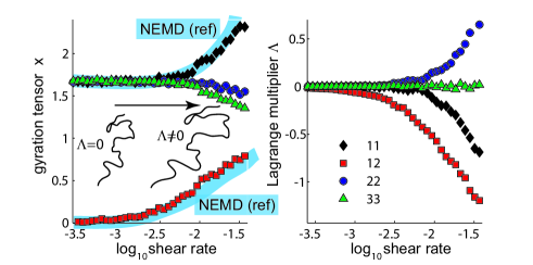
Figure 1: (color online). Components of gyration tensor ${\bf x}$ (left) and Lagrange multiplier ${\bf\Lambda}$ (right panel) vs. shear rate for a FENE polymer melt ($N=20$). Lagrange multipliers self-consistently enter the anisotropy and stretching of polymer chains. Comparison with standard NEMD reference results (left panel) show that the generalized canonical distribution (3) provides a good description of the nonequilibrium stationary state in shear flow. We use Lennard-Jones units throughout this paper.

II Original and Coarse-Grained Model System

The novel algorithm is applicable to a wide range of soft matter systems. In order to illustrate the basic idea and its worked out counterpart, let us consider a particular liquid, a classical monodisperse bulk model polymer melt. The system consists of $N_{\rm ch}$ anharmonic multibead-spring (FENE) chains made of $N$ purely repulsive Lennard-Jones beads each hoy ; mkbook ; daivis ; $N_{\rm b}=N_{\rm ch}N$ particle positions and momenta are denoted as $\{{\bf r}_{j}\}$ and $\{{\bf p}_{j}\}$. The interaction energy between particle $i$ and $j$ is $U_{ij}=U^{\rm LJ}_{ij}+U^{\rm FENE}_{ij}$, where

$$U^{\textrm{LJ}}_{ij}=4\epsilon\left[\left(\frac{\sigma}{r_{ij}}\right)^{12}-\left(\frac{\sigma}{r_{ij}}\right)^{6}+\frac{1}{4}\right]\quad\mbox{for }\ r_{ij}\leq 2^{1/6}\sigma,$$ (1)

and $U^{\textrm{LJ}}_{ij}=0$ else. The distance between particles $i$ and $j$ is denoted by $r_{ij}$, $\sigma$ the bead diameter and $\epsilon$ the Lennard-Jones interaction energy. Chain connectivity is ensured by FENE springs that act between adjacent neighbors along the chain,

$$U^{\textrm{FENE}}_{ij}=-\frac{1}{2}\epsilon_{\textrm{FENE}}\;\ln\left[1-\left(\frac{r_{ij}}{r_{0}}\right)^{2}\right],$$ (2)

and $U^{\rm FENE}_{ij}=0$ for all other particle pairs. All model parameters and thermodynamic state point are adopted from mkbook : temperature $T=\epsilon/k_{\rm B}$, density $n=0.84\,\sigma^{-3}$, finite extensibility of the springs $r_{0}=1.5\,\sigma$, and the strength of chain potential $\epsilon_{\rm FENE}=67.5\,\epsilon$ is large enough in order to prevent chain crossings. In the following, we use reduced Lennard-Jones units throughout units .

The simple FENE model system is very useful to describe the general dynamical behavior of polymer melts mkbook ; daivis ; hoy ; toddreview . This system serves as our starting point, providing the microscopic (“atomistic”) level of description without any irreversibility built in. Under the assumption that the collective variables ${{\bf\Pi}}$ capture all relevant physical processes on the time scale of interest, the nonequilibrium state of the system is characterized by the generalized canonical ensemble,

$$\rho({\bf z})=f_{\mathrm{eq}}({\bf z})\,e^{-{\bf\Lambda}:{{\bf\Pi}}({\bf z})-\Lambda_{0}},$$ (3)

with phase space coordinates ${\bf z}\equiv\{{\bf r}_{j},{\bf p}_{j}\}$ and the classical $f_{\mathrm{eq}}({\bf z})\propto\exp\{-H({\bf z})/k_{\rm B}T\}$ with $H$ denoting the microscopic Hamiltonian gellmann2007 ; hcobook2 ; ilgcanonical1 . The Lagrange multipliers ${\bf\Lambda}({\bf x})$ (cf. Fig. 1) are determined by the values of the slow variables, ${\bf x}=\langle{{\bf\Pi}}({\bf z})\rangle$, where the average is performed with (3), and $\Lambda_{0}$ a normalization constant. As structural variable, we here choose ${\bf x}$ to be the mean tensor of gyration,

$${{\bf\Pi}}({\bf z})=\frac{1}{N_{\rm ch}N}\sum_{a=1}^{N_{\rm ch}}\sum_{j=i_{a}+1}^{i_{a}+N}({\bf r}_{j}-{\bf r}_{c}^{a})({\bf r}_{j}-{\bf r}_{c}^{a}),$$ (4)

where $i_{a}=(a-1)N$ and ${\bf r}_{c}^{a}=N^{-1}\sum_{i=i_{a}+1}^{i_{a}+N}{\bf r}_{i}$ is the center of mass of chain $a$. This choice of slow variables is appropriate for low-molecular, unentangled polymeric systems, where ${\bf x}$ indeed varies slowly compared with fast relaxation processes such as fluctuation of bond lengths and angles, intermolecular distances, or higher normal modes larsonbook ; hcobook2 . For a more detailed justification of our choice of ${\bf x}$ see Appendix A. We can neglect the macroscopic hydrodynamic velocity field in (3) since it equilibrates extremely rapidly on length scales of individual polymers hco1989 . The same situation is encountered in other complex fluids as long as the large relaxation time scales of the collective variables are generated on relatively short length scales. For a more complete treatment including the hydrodynamic fields see Ref. pi_unentangled .

The time evolution for the slow variables ${\bf x}$ can in general be written as hcobook2

$$\dot{{\bf x}}=\dot{{\bf x}}_{\rm rev}+{\bf M}\,\colon\!\frac{\delta S}{\delta{\bf x}},\qquad\frac{\delta S}{\delta{\bf x}}=k_{\rm B}{\bf\Lambda},$$ (5)

where $\dot{{\bf x}}_{\rm rev}$ denotes the reversible contribution in terms of a Poisson bracket. Here, we have employed the expression for the macroscopic entropy $S({\bf x})=-k_{\rm B}\langle\ln\rho\rangle$ corresponding to the ensemble (3). Entropy gradients drive the irreversible contribution to (5). Equation (5) is justified e.g. from projection operator derivation hcoprojectors ; hcobook2 , which shows that the symmetric friction matrix ${\bf M}({\bf x})$ can be obtained from a Green-Kubo type formula

$${\bf M}=\langle\mbox{\boldmath{$\cal M$}}({\bf z}(t))\rangle,\quad\mbox{\boldmath{$\cal M$}}=\frac{1}{2k_{\rm B}\tau_{s}}\triangle_{\tau_{s}}\mbox{\boldmath{$\Pi$}}({\bf z})\triangle_{\tau_{s}}\mbox{\boldmath{$\Pi$}}({\bf z}),$$ (6)

where $\triangle_{\tau_{s}}\mbox{\boldmath{$\Pi$}}$ denotes fast fluctuations of ${{\bf\Pi}}$ on a time scale $\tau_{s}$ that separates the evolution of the slow variables ${\bf x}$ from the rapid dynamics of the remaining degrees of freedom.

The reversible part of motion is obtained analytically by considering the transformation behavior of ${{\bf\Pi}}$, cf. hcobook2 for worked out examples. Specifically, when ${\bf x}$ is a conformation tensor such as the tensor of gyration, and considering a macroscopic flow field $\mathbf{v}({\bf r})=\boldsymbol{\kappa}\cdot{\bf r}$, hence $\boldsymbol{\kappa}\equiv(\nabla\mathbf{v})^{T}$, one finds the so-called upper-convected behavior pi_unentangled , $\dot{{\bf x}}_{\rm rev}({\bf x},\boldsymbol{\kappa})={\bf x}\cdot\boldsymbol{\kappa}^{T}+\boldsymbol{\kappa}\cdot{\bf x}$. The remaining building blocks ${\bf\Lambda}$ and ${\bf M}$ needed to complete the coarse-grained model (5), we obtain self-consistently through a hybrid iteration scheme, as described next.

III Systematic Time-Scale Bridging Method

In general, the space of admissible values for the slow variable ${\bf x}$ is too large for a full parameterization of ${\bf\Lambda}({\bf x})$ from direct numerical integration. We choose to parameterize ${\bf\Lambda}$ and ${\bf M}$ along one-dimensional paths ${\bf x}(\dot{\gamma})$, where $\dot{\gamma}$ denotes the value of the external control parameter, i.e. the flow rate for chosen velocity gradients $\boldsymbol{\kappa}(\dot{\gamma})$ in our case. Note, that this procedure is analogous to the experimental determination of rheological properties in viscometric flows larsonbook . While errors in determining ${\bf\Lambda}$ can in principle violate the thermodynamic integrability condition for $S({\bf x})$, this problem is avoided when working with one-dimensional paths which do not cross. In order to calculate ${\bf\Lambda}({\bf x})$ for relevant ${\bf x}$ (here, relevant for given flow gradient $\boldsymbol{\kappa}$), we investigate nonequilibrium steady states, for which the left hand side of (5) vanishes. The systematic time-scale bridging method we propose is summarized in Tab. 1.

step	description
(i)	choose initial values for the Lagrange multipliers ${\bf\Lambda}$
(ii)	generate $n$ independent configurations distributed
	according to the generalized canonical ensemble (3)
(iii)	solve Hamilton’s unconstrained equations of motion
	for all $n$ systems during a short time interval $\tau_{s}$
(iv)	calculate the friction matrix ${\bf M}$ from Eq. (6) and
	${\bf x}$ directly from the $n$ trajectories produced in (iii)
(v)	calculate an updated value for ${\bf\Lambda}$ by solving (5)
	for ${\bf\Lambda}$ with $\dot{{\bf x}}={\bf 0}$ (in terms of ${\bf M}$, ${\bf x}$, and $\boldsymbol{\kappa}$
	the latter two quantities are “hidden” in $\dot{{\bf x}}_{\rm rev}$)

Table 1: Summary of proposed time-scale bridging method.

The updated Lagrange multipliers obtained in step (v) can potentially be used to re-enter the procedure at (i), and follow steps (ii)–(v) until ${\bf\Lambda}$ has converged. The whole procedure (i)–(v) is then repeated for other choices of the control parameter $\dot{\gamma}$ in order to establish the model (5) for different external fields.

Notice, that the strategy does not require the implementation of flow-specific boundary conditions such as Lees-Edwards (shear) mkbook or Kraynik-Reinelt (planar elongational flow) toddreview which is a particularly useful feature as it allows us to study arbitrary flow situations within exactly the same approach. In the same spirit, and in order to not potentially falsify results for the friction matrix, the algorithm also does not involve any constraints such as thermo- or barostats. These advantages are build in our approach since the macroscopic variables do not change significantly on the short time scale $\tau_{s}$ of the MD simulations in (iii).

We now specify how to implement the steps (i)–(v) efficiently, and how to self-consistently determine the range of validity of the underlying assumption (3). We choose the control parameter $\dot{\gamma}$ logarithmically equidistant, $\log(\dot{\gamma})\in[a,a+\Delta a,a+2\Delta a,..,b]$. Before we start the procedure, we initialize ${\bf\Lambda}={\bf 0}$ and $\log\dot{\gamma}=a$.

The loop starts at (i) with the current value of ${\bf\Lambda}$. For (ii) the same ${\bf\Lambda}$ is used in a MC scheme to generate microscopic configurations distributed according to (3). We have generated $n$ realizations (typically, $n=500$) by slightly modifying the procedure of hybridgeneration : For each realization, we generate $N_{\rm ch}^{\prime}>N_{\rm ch}$ (infinitely thin) independent single FENE polymer chains, each distributed according to $\exp(-{\bf\Lambda}\colon\!{{\bf\Pi}}^{*})$, where ${{\bf\Pi}}^{*}={{\bf\Pi}}/N_{\rm ch}$ is the tensor of gyration of the single chain. Next, the diameter of chains is successively increased, and overlapping chains selectively removed. With this method, we generate a polymer melt at the desired density, where the anisotropy generated by ${\bf\Lambda}$ remains preserved. Subsequently, Maxwellian distributed velocities are assigned, in agreement with (3). For (iii) one chooses a symplectic integrator (we have used a velocity-Verlet algorithm) to perform microcanonical equilibrium MD based on the microscopic Hamiltonian $H({\bf z})$. We calculate and store trajectories ${\bf z}(t)$ during a short time interval, $t\in[0,\tau_{s}]$, which is small enough to not significantly alter ${\bf x}$ during the course of the MD. For polymeric systems, the gyration tensor will relax towards equilibrium on a time scale $\tau$ which is known to be huge compared with the Lennard-Jones time unit, $\tau=0.39\,(1+N/78)N^{2}$ from mkbook for melts under study, i.e., $\tau\approx 200$ for $N=20$. As we carefully investigated, results are (as they should for proper choice of $\tau_{s}$) insensitive on $\tau_{s}$ in the regime $\tau/\tau_{s}\in[5,50]$. See also Fig. 2. We use $\tau_{s}=\tau/30\ll\tau$, and $N\in\{10,20,30\}$ for results to be presented. Notice, that the MD simulation time is thus very short compared to conventional nonequilibrium MD (NEMD) at (the problematic) low field strengths (flow rates), where simulation times large compared with the inverse rate ($\dot{\gamma}^{-1}$) are required. (iv) With the $n$ sets of phase space trajectories ${\bf z}(t)$ at hand, one inserts them into the definition of the slow variable ${{\bf\Pi}}({\bf z}(t))$, and then evaluates the friction term ${\bf M}$ (in our case a $4\times 4$ matrix) from (6), with $\triangle_{\tau_{s}}\mbox{\boldmath{$\Pi$}}({\bf z})\equiv\mbox{\boldmath{$\Pi$}}^{*}({\bf z}(\tau_{s}))-\mbox{\boldmath{$\Pi$}}^{*}({\bf z}(0))$. The average in (6) is evaluated as an arithmetic mean over the $n$ independent trajectories, e.g., ${\bf M}=(1/n)\sum_{i}\mbox{\boldmath{$\cal M$}}_{(i)}$, where we denote the partial contribution from trajectory $i\in\{1,..,n\}$ by a bracketed subscript. The number of samples $n$ has to be chosen large enough to calculate ${\bf M}$ sufficiently accurate. In our case, several components of ${\bf M}$ should vanish by symmetry consideration, and one can choose $n$ as large as to ensure these components vanish within statistical uncertainty. Notice further, that ${\bf M}$ possesses basic symmetries such as $M_{\alpha\beta\mu\nu}=M_{\mu\nu\alpha\beta}=M_{\beta\alpha\mu\nu}$ for arbitrary choices of indices because ${{\bf\Pi}}$ is symmetric. (v) Repeating the procedure (i)–(v)–(i)–.. for each $\dot{\gamma}$ until convergence can be replaced by an efficient reweighting scheme. This scheme relies on the smallness of the change of increment $\Delta a$, which comes together with moderate changes of the distribution function $\rho$. To this end we use Broyden’s method with standard settings recipes2006 which does not require the Jacobian matrix, to solve the nonlinear system

$${\bf 0}=\sum_{i=1}^{n}\left[{\bf C}_{i}+k_{\rm B}\mbox{\boldmath{$\cal M$}}_{(i)}\!\colon\!\delta{\bf\Lambda}\right]w_{i},\;w_{i}\equiv\frac{e^{-\delta{\bf\Lambda}:{{\bf\Pi}}_{(i)}}}{\sum_{j}e^{-\delta{\bf\Lambda}:{{\bf\Pi}}_{(j)}}}$$ (7)

for (matrix) $\delta{\bf\Lambda}$, with mismatch ${\bf C}_{i}\equiv\dot{{\bf x}}_{\rm rev}({{\bf\Pi}}_{(i)},\boldsymbol{\kappa})+k_{\rm B}\mbox{\boldmath{$\cal M$}}_{(i)}\!\colon\!{\bf\Lambda}$, cf. Eqs. (3), (5). For example, in a shear flow, (7) stands for six equations and six unknowns. With the solution $\delta{\bf\Lambda}$ of (7) at hand, we directly calculate the reweighted slow variables and friction matrix, ${\bf x}=\sum_{i}w_{i}{{\bf\Pi}}_{(i)}$, ${\bf M}=\sum_{i}w_{i}\mbox{\boldmath{$\cal M$}}_{(i)}$, as well as updated Lagrange multipliers, ${\bf\Lambda}\rightarrow{\bf\Lambda}+\delta{\bf\Lambda}$. A justification of the reweighting scheme is given in Appendix B. Finally, we increase the control parameter $\log\dot{\gamma}\rightarrow\log\dot{\gamma}+\Delta a$, and start over with step (i) of the procedure, until we have swept through the control parameter space.

By then, we have recorded consistent sets ${\bf x}$, ${\bf M}$, as well as ${\bf\Lambda}$ for the whole range of parameters $\dot{\gamma}$. That is, we have obtained ${\bf\Lambda}({\bf x})$ and ${\bf M}({\bf x})$ and therefore established the coarse-grained model (5) for particular parameterized path ${\bf x}(\dot{\gamma})$. By choosing the control parameters appropriately, our approach uses paths to explore those regions in state and parameter space that correspond to driven nonequilibrium situations of interest. For the system under study, the quantity ${\bf x}(\dot{\gamma})$ itself is experimentally accessible by means of small angle neutron scattering mkbook . Other particularly interesting material functions are flow curves, i.e., stress tensor $\boldsymbol{\sigma}$ as function of the control parameter $\dot{\gamma}$. The macroscopic expression for the polymer contribution to the stress tensor

$$\boldsymbol{\sigma}=-2n_{p}k_{\rm B}T\,{\bf x}\cdot\!{\bf\Lambda},$$ (8)

where $n_{p}$ is the polymer concentration, follows from both, nonequilibrium thermodynamics hcobook2 , and by evaluating the microscopic expression for the stress tensor in the ensemble (3), see Appendix C. A more detailed discussion of the stress tensor within this context is given in pi_unentangled .

Before presenting results obtained with the proposed method, we briefly comment on the time- and length-scales involved, already alluded to in the introduction. The original, microscopic model has as characteristic length scale the bead diameter $\sigma$ and reference time $\tau_{\rm LJ}=[m\sigma^{2}/\epsilon]^{1/2}$, where $m$ is the mass and $\epsilon$ the characteristic Lennard-Jones interaction energy. On the coarse-grained level, the characteristic length scale is the radius of gyration, $R_{g}\approx\sigma N^{1/2}$. The corresponding time scale estimated from the Rouse model Rouse is $\tau_{R}=\zeta(N\sigma)^{2}/[3\pi^{2}k_{\rm B}T]$, where $\zeta$ is the bead friction coefficient. Therefore, the bridging of length scale $R_{g}/\sigma=N^{1/2}$ is associated with a bridging of time scales $\tau_{R}/\tau_{\rm LJ}=cN^{2}$, where $c=5/(16\pi^{3/2})[\zeta/\zeta_{0}][\epsilon/k_{\rm B}T]^{1/2}$ with $\zeta_{0}=3\pi/(16\sigma)[\pi mk_{\rm B}T]^{1/2}$ the friction coefficient of a hard sphere gas.

IV Results

Figure 2 shows different components of the ${\bf M}$ matrix (6) as a function of the separating time $\tau_{s}$. As mentioned before, the results for ${\bf M}$ are to a good approximation independent of the precise value of $\tau_{s}$ in a broad range $\tau_{s}\in[5,50]$ which is significant smaller than the polymer relaxation time $\tau$ ($\tau\approx 200$ for $N=20$). Furthermore, the comparison in Fig. 2 shows that the simplified formula (6) approximates the more accurate integral formula hcobook2 ${\bf M}=\frac{1}{k_{\rm B}}\int_{0}^{\tau_{s}}\!{\rm d}t\langle\dot{{{\bf\Pi}}}(t)\dot{{{\bf\Pi}}}(0)\rangle$ quite well.

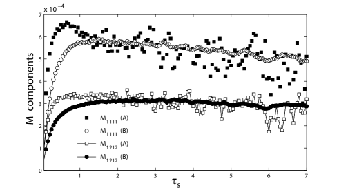
Figure 2: Different components of the friction matrix ${\bf M}$ as a function of the separating time $\tau_{s}$ obtained in step (iii) of our procedure. Solid and open symbols correspond to the integral formula mentioned in the text and Eq. (6), respectively. Results correspond to a chain length of $N=30$ and a planar shear flow with dimensionless shear rate $\dot{\gamma}=0.00036$.

Having established the thermodynamic building blocks ${\bf\Lambda}({\bf x})$ and ${\bf M}({\bf x})$, we can use the evolution equations (5) to study time-dependent flows. We have calculated transient dynamics in startup of steady shear flow, or storage and loss moduli $G^{\prime}$ and $G^{\prime\prime}$ as function of frequency $\omega$ upon using an oscillating control parameter $\dot{\gamma}\propto\sin\omega t$ (graphs not shown). We note that, due to our choice of the parameterization ${\bf x}(\dot{\gamma})$, the transient dynamics ${\bf x}(t)$ is readily calculated as long as we do not leave the known subspace $\{{\bf x}(\dot{\gamma})\}$. Otherwise, interpolation and extrapolation methods are needed for parameterizing the missing regions in ${\bf x}$-space.

There are several options to test the range of validity of the coarse-grained model. As an internal consistency check, we recommend comparing the macroscopic expression for the stress tensor Eq. (8) with the standard microscopic (virial) expression, Eq. (14). Both are available during the course of the simulation. We have verified that the two expressions for $\boldsymbol{\sigma}$ agree with each other for the range of flow rates considered. Under strong flow conditions and beyond the scope of the present study, higher order modes and kinetic contributions to the stress tensor tend to become increasingly important and need to be included suitably in ${\bf x}$, cf. ilgcanonical1 .

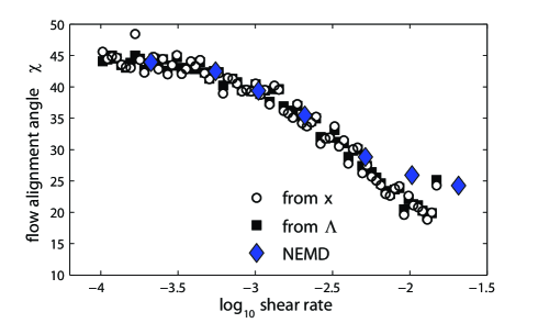
Figure 3: (color online). Flow alignment angle $\chi$ calculated from gyration tensor ${\bf x}$ (open circles) and ${\bf\Lambda}$ (filled squares) as a function of the logarithm of the shear rate $\dot{\gamma}$ for planar shear flow (chain length $N=30$). Diamonds correspond to NEMD reference results taken from mkbook obtained under the same conditions.

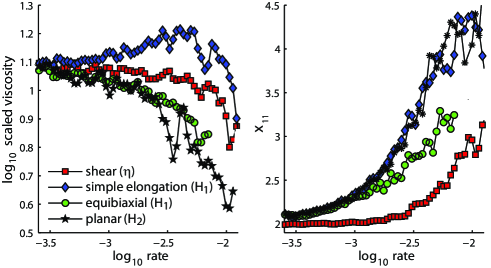
Figure 4: (color online). (a) We follow the notation employed in equibiaxial where the transposed flow gradient is written as $\nabla{\bf v}=\dot{\epsilon}\left[{\bf e}_{1}{\bf e}_{1}+m{\bf e}_{2}{\bf e}_{2}-(1+m){\bf e}_{3}{\bf e}_{3}\right]+\dot{\gamma}{\bf e}_{1}{\bf e}_{2}$, with shear rate $\dot{\gamma}$, elongation rate $\dot{\epsilon}$, special cases $m=-0.5$ (simple), $0$ (planar), $+0.5$ (elliptical), and $1$ (equibiaxial elongation) when $\dot{\gamma}=0$, and simple shear, when $\dot{\epsilon}=0$. Besides shear viscosity $\eta$, the graph shows the properly (cf. text part and equibiaxial ; daivis ) scaled viscosities $H_{1}\equiv\eta_{1}/[2(2+m)]$ and $H_{2}\equiv\eta_{2}/[2(1+2m)]$ vs. flow rate for $N=20$, where $\eta_{1}\equiv(\sigma_{11}-\sigma_{33})/\dot{\epsilon}$ and $\eta_{2}\equiv(\sigma_{22}-\sigma_{33})/\dot{\epsilon}$. (b) Maximum component of the gyration tensor ${\bf x}_{11}$ for the same types of flow, vs. flow rate ($N=20$).

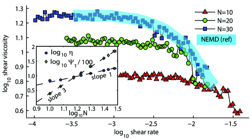
Figure 5: (color online). Polymer contribution to non-newtonian shear viscosity vs. shear rate for various molecular weights. Exemplarily, reference results obtained via direct NEMD simulation mkbook are shown for $N=30$. The inset shows zero-rate shear viscosity $\eta_{0}$ and first viscometric function $\Psi_{1,0}$ vs. chain length $N$, both coinciding with data from extensive NEMD mkbook .

We apply the proposed method to the FENE polymer melt described above, subjected to various flows (results for mixed and elliptical elongational flow not shown). For the case of simple shear, Fig. 1 shows the shear rate dependence of the chosen slow variable ${\bf x}$ (tensor of gyration in our case) and the corresponding Lagrange multiplier ${\bf\Lambda}$. Very good agreement of ${\bf x}$ with NEMD reference results is obtained. As a further consistency check, we have verified, that the basic identity $(x_{11}-x_{22})x_{12}^{-1}=(\Lambda_{11}-\Lambda_{22})\Lambda_{12}^{-1}$, derived from Eq. (5) vlasisPRL2007 using our choice for ${\bf x}$ and $\boldsymbol{\kappa}$, holds within error margins. This quantity is related to the flow alignment angle $\chi$ by $(x_{11}-x_{22})x_{12}^{-1}=2\cot(2\chi)$. Therefore, we show in Fig. 3 the alignment angle $\chi$ calculated from ${\bf x}$ as well as from ${\bf\Lambda}$. The very good agreement between those values shows the intrinsic consistency of our results. Furthermore, our results are also in good agreement with standard NEMD simulation also displayed in Fig. 3 for planar shear flow with $N=30$ mkbook . Figure 4a shows shear and extensional viscosities for different flow conditions. Our results confirm expectations from a retarded motion expansion analysis for a comparable system, studied via extensive NEMD in daivis . In particular, Fig. 4a shows that the scaled viscosities all superimpose for vanishing flow rates, in agreement with predictions from linear viscoelasticity theory. Also in agreement with previous results, the viscosity in simple elongation exhibits a maximum around a dimensionless rate of order unity, while in planar and equibiaxial elongation as well as in planar shear flow the viscosity decreases monotonically with flow rate equibiaxial ; daivis . The corresponding $x_{11}$-components of the gyration tensor, which characterize the polymer stretch, are plotted in Fig. 4b. We observe that polymer stretching is much more pronounced for planar and equibiaxial elongation compared to in planar shear flow. We have further validated the proposed algorithm for the rate ($\dot{\gamma}$) and chain length ($N$) dependence of the shear viscosity (see Fig. 5, which offers a quantitative comparison with available NEMD data from mkbook for an identical system). Since our method does not require flow-adapted boundary conditions, we are able to include here the first simulation results on steady state equibiaxial elongation. All results for the sample application, including the many beyond the scope of this article and therefore not reported here, reproduce available experimental findings for gyration tensor and viscosities (shear thinning, strain hardening only in simple elongation, alignment in shear weaker than in elongation at same flow invariants, scaling behavior, overshoots, cf. larsonbook ; equibiaxial ; dealybook ). The results provided in this section clearly demonstrate that the proposed simple procedure outlined in Tab. 1 allows to (i) recover known results obtained via classical approaches, (ii) study flow geometries not accessible using alternate approaches, (iii) calculate the friction matrix and Lagrange multiplier, i.e., the irreversible part of the closed and low-dimensional time evolution equation (5) for the coarse-grained variable in a straightforward manner.

V Conclusions

Using an alternating MC–MD iteration scheme, our approach successfully bridges the time-scale gap between microscopic and macroscopic scales by establishing the coarse-grained model within a nonequilibrium thermodynamics framework. Since only short MD simulations are needed, our method is very efficient (moreover, it is ideally suited for parallelization) and particularly allows to deal with arbitrary flow gradients, since neither special boundary conditions nor other constraints are needed. To be specific, even from the viewpoint of material property determination, our method is more efficient than standard NEMD when $\dot{\gamma}\tau<(n_{0}/n)(\tau/\tau_{s})$, where $n_{0}$ denotes the number of strain units needed for the NEMD. With $\tau/\tau_{s}=30$, $n=500$ used here, taking $n_{0}=10$ from daivis and also the time for the MC step into account (see hybridgeneration ), our method is superior to NEMD for $\dot{\gamma}\tau\leq 0.5$, and $m$ orders of magnitude faster at a value $10^{m}$ times smaller than that dimensionless rate.

The presented approach is very general, but the (a-posteriori validated) success of the coarse-graining procedure depends crucially on the proper choice of the slow variable. As mentioned above in our illustrating example, conformation tensors as slow variables for polymer melts are clearly restricted to the unentangled regime because interchain effects, entanglements or knots, hinder the relaxation of the conformation tensor for high molecular weight polymers hoy ; mkbook . Some promising candidates for other soft matter systems are the tensorial order parameter for liquid crystals, the magnetization for magnetic liquids, and the path length of the entanglement network for entangled polymer melts larsonbook ; mkbook ; christoscurropin . The MC step is particularly challenging for dense polymeric systems, but efficient schemes exist for FENE as well as for atomistic models vlasisPRL2007 ; nikosPRL2002 .

For many complex fluids, Eq. (3) is known to serve as a successful starting point to derive closure relationships mkbook ; ilgcanonical1 . Therefore, our method establishes the coarse-grained model all the way from equilibrium up to the validity of (3) and complements standard NEMD methods, which remain often well-suited for the less challenging regime of strong external forcing.

Appendix A Choice of slow variables

The proper choice of appropriate slow (collective) variables is crucial not only for the method proposed here but for a broad class of nonequilibrium statistical mechanics approaches based on projection operator techniques hcobook2 .

In the present case of unentangled polymer melts, there is ample evidence that single chain conformation tensors are promising candidates for slow variables larsonbook ; hcobook2 ; vlasisPRL2007 . Therefore, we assume the slow variable ${\bf x}$ can be decomposed into an average over single chain (symmetric second rank) conformation tensors,

$${\bf x}=\frac{1}{N_{\rm ch}}\sum_{a=1}^{N_{\rm ch}}{\bf x}^{(a)}.$$ (9)

The latter can always be expanded in a series of Rouse modes,

$${\bf x}^{(a)}=\sum_{p=1}^{N-1}c_{p}{\bf X}_{p}^{(a)}{\bf X}_{p}^{(a)};\quad{\bf X}_{p}^{(a)}=\sum_{j=1}^{N-1}\Omega_{pj}{\bf Q}_{j}^{(a)},$$ (10)

where ${\bf X}_{p}^{(a)}$ is the $p$-th Rouse mode of chain $a$, $\Omega_{pj}=\sqrt{2/N}\sin(p\pi j/N)$ an element of the Rouse matrix and ${\bf Q}_{j}^{(a)}$ the connector vector of particles $j+1$ and $j$ of chain $a$ larsonbook .

As possible choice of the weights $c_{p}$ in Eq. (10), we initially implemented $c_{p}=\delta_{p1}$, i.e. only the first Rouse mode is included. This choice is reasonable since the first Rouse mode is the slowest and therefore a natural candidate for the slow variable ${\bf x}$. However, the resulting model is restricted to very small deviations from equilibrium because there is no clear time scale separation to the higher modes which are neglected. In fact, the relaxation time of mode $p$ in the Rouse model is $\tau_{p}=\zeta/[8k\sin^{2}(p\pi/2N)]\propto\tau_{1}/p^{2}$ ($\zeta$ and $k$ are the bead friction coefficient and the spring constant in the Rouse model, respectively) and therefore the second mode relaxes only a factor four faster than the first one. Thus, when driven out of equilibrium like in a flow situation, several of the lowest Rouse modes are typically excited. In order to address this issue, we propose to include all Rouse modes in a single quantity such that the increasing relaxation times of the higher modes are reflected in a decreasing weight $c_{p}$. Such a choice can be motivated by the fact that, in a stationary flow situation, the Lagrange multiplier is proportional to the product of relaxation time and velocity gradient (see e.g. Eq. (8.52) in hcobook2 ). Thus, we use a single Lagrange multiplier ${\bf\Lambda}$ in the nonequilibrium ensemble Eq. (3) in order to excite all Rouse modes at the same time in a way that is consistent with Rouse theory. With $c_{p}=N/(\pi p)^{2}$ decreasing for increasing mode number $p$ as the corresponding relaxation times, ${\bf x}$ becomes the gyration tensor, at least to a very good approximation. Comparing different choices for ${\bf x}$ (gyration tensor and the second rank tensor formed by either the first Rouse mode or the end-to-end vector), we found the gyration tensor to give the most accurate results.

Appendix B Reweighting scheme

We here describe the reweighting scheme employed in the above described algorithm. The generalized canonical distribution (3) is denoted by $\rho_{\Lambda}({\bf z})$, in order to make explicit its dependence on the values of the Lagrange multipliers ${\bf\Lambda}$. Corresponding averages of phase space functions are $\langle A\rangle_{\Lambda}\equiv\int\!{\rm d}{\bf z}\,A({\bf z})\rho_{\Lambda}({\bf z})$. The analytical form of (3) allows to relate the distribution $\rho_{\Lambda+\delta\Lambda}({\bf z})$ corresponding to different Lagrange multipliers ${\bf\Lambda}+\delta{\bf\Lambda}$ to $\rho_{\Lambda}({\bf z})$ by

$$\rho_{\Lambda+\delta\Lambda}({\bf z})=\rho_{\Lambda}({\bf z})\,\frac{e^{-\delta{\bf\Lambda}:{{\bf\Pi}}({\bf z})}}{\left\langle e^{-\delta{\bf\Lambda}:{{\bf\Pi}}({\bf z})}\right\rangle_{\Lambda}}.$$ (11)

Therefore, also the averages of phase space functions corresponding to different values of Lagrange multipliers are related by

$$\left\langle A\right\rangle_{\Lambda+\delta\Lambda}=\frac{\left\langle Ae^{-\delta{\bf\Lambda}:{{\bf\Pi}}({\bf z})}\right\rangle_{\Lambda}}{\left\langle e^{-\delta{\bf\Lambda}:{{\bf\Pi}}({\bf z})}\right\rangle_{\Lambda}}.$$ (12)

For small deviations $\delta\Lambda$, the latter expression simplifies to

$$\left\langle A\right\rangle_{\Lambda+\delta\Lambda}\approx\frac{\left\langle A\right\rangle_{\Lambda}-\delta{\bf\Lambda}:\left\langle{{\bf\Pi}}A\right\rangle_{\Lambda}}{1-\delta{\bf\Lambda}:\left\langle{{\bf\Pi}}\right\rangle_{\Lambda}}.$$ (13)

Equation (12) or (13) for $A={{\bf\Pi}}$ and $A=\mbox{\boldmath{$\cal M$}}$ are used in the reweighting scheme in order to calculate the corrected values for ${\bf x}$ and ${\bf M}$, respectively, from recorded averages. In principle, Eq. (12) allows to recalculate averages of $A$ for arbitrary $\delta{\bf\Lambda}$. In practice, however, due to the finite ensemble size, such estimates are accurate only if $\rho_{\Lambda}$ and $\rho_{\Lambda+\delta\Lambda}$ have considerable overlap. This is the case for $\delta{\bf\Lambda}$ small enough such that relevant states for averages at ${\bf\Lambda}+\delta{\bf\Lambda}$ are sufficiently well sampled with $\rho_{\Lambda}$.

Appendix C Stress tensor in generalized canonical ensemble

Point of departure is the microscopic expression for the total stress tensor larsonbook which can be inferred from the term of second order in the expansion of the configurational Helmholtz free energy with respect to the strain tensor Hess97

$$\sigma_{\alpha\beta}^{\rm tot}=-\frac{1}{V}\left\langle\sum_{j}m_{j}c_{j,\alpha}c_{j,\beta}\right\rangle-\frac{1}{V}\left\langle\sum_{j}r_{j,\alpha}F_{j,\beta}\right\rangle.$$ (14)

The first, kinetic contribution can be well approximated by the ideal gas expression with $p\equiv nk_{\rm B}T$. Deviations from this expression are minor in polymer melts and show up only at extremely high flow rates mkbook ; mk_chainend .

We further assume (i) potential forces $F_{j,\alpha}=-\partial H/\partial r_{j,\alpha}$, and (ii) a generalized canonical ensemble $\rho(z)=(1/Z^{\ast})\exp[-\beta H-N_{\rm ch}{\bf\Lambda}\colon{{\bf\Pi}}]$, cf. Eq. (3), where $N_{\rm ch}$ denotes the number of polymer chains.

Assumptions (i) and (ii) allow us to write

$$F_{j,\beta}\,\rho = -\frac{\partial H}{\partial r_{j,\beta}}\rho$$ (15)

$$= \frac{1}{\beta}\frac{\partial}{\partial r_{j,\beta}}\rho+\frac{N_{\rm ch}}{\beta}\Lambda_{\mu\nu}\frac{\partial\Pi_{\mu\nu}}{\partial r_{j,\beta}}\rho.$$

Inserting this into (14) gives

$$\sigma_{\alpha\beta}^{\rm tot} = -p\delta_{\alpha\beta}-\frac{1}{\beta V}\sum_{j}\underbrace{\int\!{\rm d}{\bf z}\,r_{j,\alpha}\frac{\partial}{\partial r_{j,\beta}}\rho({\bf z})}_{=0}$$ (16)

$$-\frac{N_{\rm ch}\Lambda_{\mu\nu}}{V\beta}\sum_{j}\int\!{\rm d}{\bf z}\,r_{j,\alpha}\frac{\partial\Pi_{\mu\nu}}{\partial r_{j,\beta}}\rho({\bf z})$$

$$= -p\delta_{\alpha\beta}-n_{p}k_{\rm B}T\Lambda_{\mu\nu}\left\langle\sum_{j}r_{j,\alpha}\frac{\partial\Pi_{\mu\nu}}{\partial r_{j,\beta}}\right\rangle.$$

For the special case of conformation tensor models, ${{\bf\Pi}}$ can be expressed as a bilinear form of the particle positions. Then, we obtain from Eq. (16) the final expression

$$\boldsymbol{\sigma}^{\rm tot}=-p{\bf 1}-2n_{p}k_{\rm B}T{\bf x}\cdot{\bf\Lambda}.$$ (17)

Equation (17) can independently be derived from nonequilibrium thermodynamics hcobook2 . It should be noted that Eq. (17) captures the polymer contribution to the stress tensor as the Lagrange multipliers ${\bf\Lambda}$ describe nonequilibrium polymer configurations. For short-chain polymer melts, a “simple fluid contribution” has to be added in order to account for the stress contribution to the total stress tensor that would be present in the absence of chain connectivity Barrat_Rouse ; pi_unentangled .

References

- (1) M. Gell-Mann, J. B. Hartle, Phys. Rev. A 76, 022104 (2007).
- (2) R. G. Larson, The structure and rheology of complex fluids (Oxford University Press, New York, 1999).
- (3) C. Pierleoni, C. Addison, J.-P. Hansen, V. Krakoviack, Phys. Rev. Lett. 96, 128302 (2006).
- (4) S. O. Nielsen, C. F. Lopez, G. Srinivas, M. L. Klein, J. Phys.: Condens. Mat. 16, R481 (2004).
- (5) J. Baschnagel et al., Adv. Polym. Sci. 152, 41 (2000).
- (6) M. Praprotnik, L. D. Site, K. Kremer, Ann. Rev. Phys. Chem. 59, 545 (2008).
- (7) M. G. Guenza, J. Phys.: Condens. Mat. 20, 033101 (2008).
- (8) S. Curtarolo, G. Ceder, Phys. Rev. Lett. 88, 255504 (2002).
- (9) R. G. Larson, Mol. Phys. 102, 341 (2004).
- (10) R. L. C. Akkermans, W. J. Briels, J. Chem. Phys. 114, 1020 (2001).
- (11) J. T. Padding, W. J. Briels, J. Chem. Phys. 117, 925 (2002).
- (12) H. C. Öttinger, MRS Bull. 32, 936 (2007).
- (13) H. C. Öttinger, Beyond Equilibrium Thermodynamics (Wiley, Hoboken NJ, 2005).
- (14) M. Kröger, W. Loose, S. Hess, J. Rheol. 37, 1057 (1993); Phys. Rev. Lett. 85, 1128 (2000); M. Kröger, Models for Polymeric and Anisotropic Liquids (Springer, Berlin, 2005).
- (15) P. J. Daivis, M. L. Matin, B. D. Todd, J. Non-Newton. Fluid Mech. 147, 35 (2007); ibid. 111, 1 (2003).
- (16) K. Kremer, G. S. Grest, J. Chem. Phys. 92, 5057 (1990); R. S. Hoy, G. S. Grest, Macromolecules 40, 8389 (2007).
- (17) Reduced units - online interactive tool permanently available at http://www.complexfluids.ethz.ch/units
- (18) B. D. Todd, P. J. Daivis, Mol. Simul. 33, 189 (2007); Phys. Rev. Lett. 81, 1118 (1998).
- (19) P. Ilg, I. V. Karlin, H. C. Öttinger, Physica A 315, 367 (2002).
- (20) H. C. Öttinger, Y. Rabin, J. Rheol. 33, 725 (1989).
- (21) P. Ilg, Physica A 387, 6484 (2008).
- (22) H. C. Öttinger, Phys. Rev. E 57, 1416 (1998).
- (23) M. Kröger, Comput. Phys. Commun. 118, 278 (1999).
- (24) W. H. Press, S. A. Teukolsky, W. T. Vetterling, B. P. Flannery, Numerical Recipes. The art of scientific computing, 3rd. Ed. (Cambridge University Press, NY, 2006).
- (25) P. E. Rouse, J. Chem. Phys. 21, 1272 (1953).
- (26) C. Baig, V. G. Mavrantzas, Phys. Rev. Lett. 99, 257801 (2007).
- (27) P. Hachmann, J. Meissner, J. Rheol. 47, 989 (2003).
- (28) J. M. Dealy, R. G. Larson, Structure and Rheology of Molten Polymers (Hanser, Munich, 2006).
- (29) C. Tzoumanekas, D. N. Theodorou, Curr. Opin. Solid State Mater. Sci. 10, 61 (2006).
- (30) N. Ch. Karayiannis, V. G. Mavrantzas, D. N. Theodorou, Phys. Rev. Lett. 88, 105503 (2002).
- (31) S. Hess, M. Kröger, W. G. Hoover, Physica A 239, 449 (1997).
- (32) M. Kröger, S. Hess, Physica A 195, 336 (1993).
- (33) M. Vladkov, J.-L. Barrat, Macromol. Theory Simul. 15, 252 (2006).