The non-equilibrium dynamics of an amorphous solid is studied with a soft-spin type model. We show that the aging behavior in the glassy state follows a modified Kohlrausch-Williams-Watts (KWW) form similar to that obtained in Phys. Rev. Lett. 95, 055702 (2005) from analysis of the dielectric loss data. The nature of the fluctuation-dissipation theorem (FDT) violation is also studied in the time as well as correlation windows.

Nonequilibrium dynamics in an amorphous solid

In the glassy state, the liquid behaves like a frozen solid with the motion of its constituent particles being localized around randomly distributed sites. Analysis of the dynamics in this non equilibrium glassy state reveals a variety of phenomena like aging and memory effects ediger ; struik . Important progress in understanding the non equilibrium dynamics of disordered systems has been made in recent years from study of simple mean field spin glass models. In the multi-spin interaction models, the non-linearities in the Langevin dynamics give risetrk to a ergodic-nonergodic transition. The basic mechanism for this transition is very similar to that present in the models for the dynamics of supercooled liquidsrmp . The seminal work of Ref. cugli dealt with the problem of weak ergodicity breakingbouchaud in a spherical $p$-spin ($p>2$) interaction modelsoomers over the asymptotic time scales. Here the crossing over of the dynamics from a regime of time translational invariance to that of aging behavior was demonstrated analytically. Low temperature properties of glassy systems, e.g., thermal conductivity and specific heat, have also been studied with models kuhn for the structural glass in terms of a standard Hamiltonian involving spins. In the present paper, we study a soft-spin type model, which is defined in terms of the displacements of the particles around a corresponding set of random lattice points. We show that the aging behavior in the nonequilibrium glassy state follows a modified KWW form similar to that obtained in Ref. loidl from analysis of the dielectric loss data for several materials below the glass transition temperature $T_{g}$.

We consider a model Hamiltonian, which has a translationally invariant form in terms of the displacement variables $u_{i}$ around an amorphous structure.

$$H=\sum_{p=2}^{\infty}\sum_{i\neq{j}}J^{(p)}_{ij}(u_{i}-u_{j})^{p}~{}~{}.$$ (1)

For the amorphous solid, the interaction matrix $J^{(p)}_{ij}$ is assumed to be random following a gaussian probability distribution of zero mean and variance $J_{p}^{2}/N$. The microscopic basis for such a model for an amorphous solid is discussed further below. The time evolution of $u_{i}(t)$ is given by the dissipative Langevin equation,

$$\Gamma_{0}^{-1}\frac{\partial u_{i}}{\partial t}~{}=~{}-\beta\frac{\delta H}{\delta u_{i}}-z(t)u_{i}+\xi_{i}(t).$$ (2)

$\Gamma_{0}$ is the bare kinetic coefficient related to the variance of the gaussian white noise $\xi_{i}$ through the fluctuation-dissipation relation $<\xi_{i}(t)\xi_{j}(t^{\prime})>~{}=~{}2\beta^{-1}\Gamma_{0}\delta_{ij}\delta(t-t^{\prime})$. $z(t)$ is a Lagrange’s multiplier used enforcing the constraint $N^{-1}\sum_{i}<u_{i}^{2}(t)>=1$. This in the present context is equivalent to having a constant Lindemann parameter at a fixed temperature $T$. The simplest form of the nonlinear Langevin equation (2) is obtained by keeping in $H$ the contributions from the $p=2$ and $3$ terms of the expansion (1). In the present work, we focus on the corresponding nonlinear model for the dynamics and refer this as the p23 model from hereon.

We formulate a standard Martin-Siggia-Rose (MSR) msr field theory to compute the time correlation and response functions of the displacement variable $u_{i}$. The field $\hat{u}_{i}$ conjugate to $u_{i}$ is introduced in this regard to average over the gaussian noise $\xi_{i}$. The two time correlation and response functions are respectively defined as : $C(t,t_{\mathrm{w}})=N^{-1}\sum_{i=1}^{N}\overline{\left<u_{i}(t)u_{i}(t_{\mathrm{w}})\right>}$, and $R(t,t_{\mathrm{w}})=N^{-1}\sum_{i=1}^{N}\overline{\left<\hat{u}_{i}(t)u_{i}(t_{\mathrm{w}})\right>}$, where the overbars stand for averages over the random bonds $\{J^{(p)}_{ij}\}$’s and the angular brackets represent mean over the gaussian white noise $\xi_{i}$’s. The dynamics of the correlation and response functions are obtained from the equations

$$\left[{\partial}_{t}+z(t)\right]C(t,t_{\mathrm{w}}) = \int_{0}^{t}ds\Sigma(t,s)C(s,t_{\mathrm{w}})+\int_{0}^{t_{\mathrm{w}}}ds~{}\Xi^{\prime}(t,s)R(t_{\mathrm{w}},s)$$ (3)

$$\left[{\partial}_{t}+z(t)\right]R(t,t_{\mathrm{w}}) = \delta(t-t_{\mathrm{w}})+\int_{t_{\mathrm{w}}}^{t}ds\Sigma(t,s)C(s,t_{\mathrm{w}}),$$ (4)

where we denote $\Xi^{\prime}(t,t^{\prime})=2\delta(t-t^{\prime})+\Xi(t,t^{\prime})$. The kernels are obtained from a perturbative summation as $\Xi(t,t^{\prime})=\sum_{p}a_{p}C^{p-1}(t,t^{\prime}),$ and $\Sigma(t,t^{\prime})=\sum_{p}(p-1)a_{p}C^{p-2}(t,t^{\prime})R(t,t^{\prime})$ in terms of a set of coupling constants $\{a_{p}\}$, which depend on nonlinearities in the dynamic equations. For the $p23$ model, we obtain up to one loop order $a_{2}=2{(\beta J_{2})}^{2}$ and $a_{3}=18{(\beta J_{3})}^{2}$. The necessary boundary conditions for $C$ and $R$ are respectively chosen ascugli : $R(t,t^{-})=1$ and $\partial_{t}C(t,t^{\pm})=\pm 1$. The Lagrange’s multiplier $z(t)$, which ensures $C(t,t)=1$, is obtained as $z(t)=1+\int_{0}^{t}ds\left\{\Xi(t,s)R(s,t)+\Sigma(t,s)C(t,s)\right\}$.

The analysis of the asymptotic dynamics of $C(t,t_{\mathrm{w}})$ for both $t$ and $t_{\mathrm{w}}\rightarrow\infty$ is dividedcugli into two main regimes. First, for $(t-t_{\mathrm{w}})/t\rightarrow 0$ the time translational invariance (TTI) holds. At this stage $C$ and $R$ are related through the fluctuation dissipation theorem (FDT) $R_{\mathrm{I}}(t)=-\Theta(t)\partial_{t}C_{\mathrm{I}}(t)$, where we denote $C(t+t_{\mathrm{w}},t_{\mathrm{w}}){\equiv}C_{\mathrm{I}}(t)$ and $R(t+t_{\mathrm{w}},t_{\mathrm{w}}){\equiv}R_{\mathrm{I}}(t)$. Second, for $(t-t_{\mathrm{w}})/t\sim 1$, i.e., for widely separated $t$ and $t_{\mathrm{w}}$ there is aging behavior. The correlation and response functions, respectively denoted by $C_{\mathrm{A}}$ and $R_{\mathrm{A}}$ in this case, are assumed to be functions of $t_{\mathrm{w}}/t\equiv\lambda$ $(0<\lambda<1)$. We define $C_{A}(t,t_{\mathrm{w}})=q{\cal C}(\lambda)$ and $R_{A}(t,t_{\mathrm{w}})=t^{-1}{\cal R}(\lambda)$. In the limit, $\lambda\rightarrow{1}$, ${\cal C}(\lambda)\rightarrow{1}$ and ${\cal R}(\lambda)\neq{0}$. The solutions in the FDT and the aging regimes agree if the long time limit of $C_{\mathrm{I}}(\tau)$ is $q$ termed as the non ergodicity parameter (NEP). In the FDT regime, both the eqns. (3) and (4) reduce to a single equation

$$\left({\partial}_{t}+1\right)C_{\mathrm{I}}(t)+\int_{0}^{t}ds\Xi_{F}(t-s)\partial_{s}C_{\mathrm{I}}(s)=z_{\infty}[C_{\mathrm{I}}(t)-1].$$ (5)

The kernel $\Xi_{I}[C_{\mathrm{I}}]$ reduce to $a_{2}C_{\mathrm{I}}+a_{3}C_{\mathrm{I}}^{2}$ in case of the p23 model. Except for the linear term on the RHS, eqn. (5) is same as the basic dynamical equation in the self-consistent mode-coupling theory of the structural glass. The latter represents the asymptotic dynamics for the time correlation of the equilibrium density fluctuations in a supercooled liquid. However, in the present case the nontrivial renormalization contribution to the transport coefficient comes from the dissipative nonlinearities in (2), while in the MCT for compressible liquids the relevant nonlinearity is in the reversible pressure term. From the $t\rightarrow\infty$ limit of eqn. (5) we obtain the following relation

$$\sum_{p}a_{p}(p-1)q^{p-2}+{(1-q)}^{2}=0~{}~{}.$$ (6)

for the NEP $q$ in terms of the coupling constants $a_{p}$ .

In the aging regime, the FDT violation is denoted in terms of a parameter $m$, which is defined through the relation $R_{\mathrm{A}}(t)=-m\Theta(t)\partial_{t}C_{\mathrm{A}}(\tau)$ or equivalently ${\cal R}(\lambda)=-mq(\partial/\partial\lambda){\cal C}(\lambda)$. We obtain analyzing eqns. (3) and (4) in the aging regime, the following equations for $m$ and $q$,

$$m=(1-q){{\sum_{p}a_{p}(p-2)q^{p-2}}\over{\sum_{p}a_{p}q^{p-1}}}$$ (7)

At the transition $m=1$. The critical coupling constants $\{a_{2}^{*},a_{3}^{*}\}$ for dynamic transition point of the p23 model is obtained from the solution of eqns. (6) and (7) as $a^{*}_{2}=2/\lambda_{0}-1/\lambda_{0}^{2}$ and $a^{*}_{3}=1/\lambda_{0}^{2}$, where $\lambda_{0}=1-q$. The ergodic-nonergodic transition line is given by $a^{*}_{2}=2\sqrt{a^{*}_{3}}-a^{*}_{3}$. This is identical to the line of dynamic transition in the $\phi_{12}$ modelgoetze ; kim-mazenko of the mode coupling theory of structural glass transition. Along the line of transition the parameter $\lambda_{0}$ changes from $0$ to $0.5$ as the NEP changes from 1 to 0. In the ergodic phase, the NEP $q=0$ and the FDT holds with $m=1$. Close to the transition line, the relaxation behavior follows several regimes crossing over from power law decay to a final stretched exponential form. The corresponding stretching exponent $\beta_{\alpha}^{E}$ is approximatedkim-mazenko with the empirical relation $\sum_{p}a_{p}qp^{-1/{\beta_{\alpha}^{E}}}=1$.

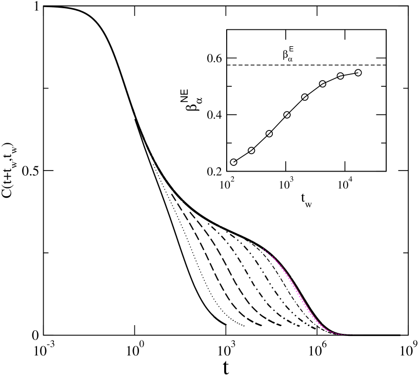
Figure 1: The correlation $C(t+t_{\mathrm{w}},t_{\mathrm{w}})$ vs. $t$ for a set of waiting times $t_{\mathrm{w}}$’s in the ergodic phase, $a_{2}=.82$ and $a_{3}=2.0$. Inset shows the exponent $\beta_{\alpha}$ for final stretched exponential relaxation w.r.t. $t_{\mathrm{w}}$. Dashed line is the corresponding equilibrium value of stretching exponent.

To get a better understanding of the time scales associated with the aging dynamics in the intermediate time regime and the corresponding FDT violation, we solve the eqns. (3) and (4) numerically. This requires integrating the equations (3) and (4) for both $t$ and $t_{\mathrm{w}}$ extending over several time decades. We use the adaptive integration technique berthier , which starts with smaller sized grids for integration over shorter time scales of fast relaxation and correspondingly increases the step size for longer time scales of slow dynamics. In the ergodic state, at long waiting times $t_{\mathrm{w}}$ the correlation function approaches its equilibrium value and time translational invariance is eventually reached. In the approach to the equilibrium, the waiting time dependence of $C(t+t_{\mathrm{w}},t_{\mathrm{w}})$ is displayed w.r.t. $t$ in fig. 1 for $a_{2}=0.82$ and $a_{3}=2.02$. In the final stage, the decay follows the stretched exponential form $\exp[-(t/\tau^{NE}_{\alpha})^{\beta^{NE}_{\alpha}}]$ with characteristic relaxation time $\tau^{NE}_{\alpha}$ and stretching exponent $\beta^{NE}_{\alpha}$. The inset of fig. 1 shows $\beta^{NE}_{\alpha}$ corresponding to different waiting times $t_{\mathrm{w}}$. At large $t_{\mathrm{w}}$, it approaches its equilibrium value $\beta_{\alpha}^{E}$, which is determined in terms of $a_{2}$ and $a_{3}$ using the empirical relation discussed above.

In the non-ergodic state, the numerical solution of eqns. (3) and (4) displays both FDT and aging behavior. In fig.2, the time dependence of $C(t+t_{\mathrm{w}},t_{\mathrm{w}})$ corresponding to $a_{2}=0.5$ and $a_{3}=6.0$ deep in the glassy state are shown for different values of $t_{\mathrm{w}}$. Initially the correlation decays from $1$ to $q$ and at this stage time translational invariance holds. The dynamics is strongly dependent on $t_{\mathrm{w}}$ at a later stage. The corresponding correlation and response functions for large $t_{\mathrm{w}}$ are scaled with the ansatz : $C(t+t_{\mathrm{w}},t_{\mathrm{w}})=C[h(t+t_{\mathrm{w}})/h(t_{\mathrm{w}})]$ where $h(t)$ is a monotonically ascending function of $t$. The simplest possibility $h(t)=t^{\gamma}$ is termed as the simple aging and implies $C(t,t_{\mathrm{w}})\equiv C(t/t_{\mathrm{w}})$. We adopt here the more general formvincent ; kim-latz $h(t)=\exp[t^{1-\kappa}/(1-\kappa)]$. The limit $\kappa{\rightarrow}0$ implies time translational invariance while $\kappa{\rightarrow}1$ represents simple aging. The case $0<\kappa<1$ is termed as sub-aging. The dynamics almost conforms to simple aging behavior as shown in the inset of fig.2 in which different $t_{\mathrm{w}}$ data overlap on a single master curve having $\kappa=0.96$. For every $t_{\mathrm{w}}$, the correlation $C(t+t_{\mathrm{w}},t_{\mathrm{w}})$ decays to zero at sufficiently long $t$. This is termed as weak ergodicity breaking in the aging regime.

We now focus on the aging time dependence of the relaxation. For a set of $t_{\mathrm{w}}$’s, the fourier transform of the correlation function $C(t+t_{\mathrm{w}},t_{\mathrm{w}})$ with respect to $t$ is obtained numerically. Since the correlation function in the aging regime is approximately function of $t/t_{\mathrm{w}}$ ($\kappa=.96$), the corresponding fourier transform $C(\omega,t_{\mathrm{w}})$ is a function of ${\omega}t_{\mathrm{w}}\equiv\tilde{t}_{\mathrm{w}}$. For comparison with experimental data, we define the response function $\chi_{\omega}(\tilde{t}_{\mathrm{w}})\equiv\omega C(\omega,t_{\mathrm{w}})$. The waiting time ($\tilde{t}_{\mathrm{w}}$) dependences of $\chi_{\omega}(\tilde{t}_{\mathrm{w}})$ for different frequencies do not fit with a simple stretched exponential form $\exp[-(t/\tau)^{\beta}]$ with constant $\tau$ over the whole time range and a frequency independent $\beta$. The data is fitted with the modified KWW in a manner similar to that of Ref. loidl .

$$\chi_{\omega}(\tilde{t}_{\mathrm{w}})=\left[\chi^{\mathrm{st}}_{\omega}-\chi^{\mathrm{eq}}_{\omega}\right]\exp\left[-({\tilde{t}_{\mathrm{w}}}/\tau(\tilde{t}_{\mathrm{w}}))^{\beta}\right]+\chi^{\mathrm{eq}}_{\omega}$$ (8)

where the subscripts ”st” and ”eq” respectively refer to the limits $\tilde{t}_{\mathrm{w}}\rightarrow 0$ and $\infty$ for $\chi_{\omega}$. The aging time dependence of $\tau$ is chosen as

$$\tau(\tilde{t}_{\mathrm{w}})=\left\{\tau_{\mathrm{st}}-\tau_{\mathrm{fn}}\right\}f(\tilde{t}_{\mathrm{w}})+\tau_{\mathrm{fn}}~{}~{},$$ (9)

where $\tau_{\mathrm{st}}$ and $\tau_{\mathrm{fn}}$ are fit parameters independent of frequency $\omega$. The normalized function $f(s)$ is chosen to have limiting values $1$ and $0$ for $s\rightarrow{0}$ and $\infty$ respectively. In particular, we make the choicesengupta $f(s)=a_{o}/[1+\exp{\{s/\tau(s)\}}^{\beta}]$ where $a_{0}=2^{\beta}$ is a normalization constant. Using this form of the $\tau(\tilde{t}_{\mathrm{w}})$ we have fitted $\chi_{\omega}(\tilde{t}_{\mathrm{w}})$ for all the different frequencies with a single ( frequency independent ) stretching exponent $\beta$. In fig. 3, a scaled plot of the different frequency data with respect to $\tilde{t}_{\mathrm{w}}$ is displayed. The data sets for all the frequencies merge on a single master curve with $\beta=0.55$ and is shown as a solid line. For the dielectric loss data, Lunkenheimer et. al. in Ref. loidl use a somewhat different fitting scheme with the $f(s)$ in eqn. (9) being a stretched exponential function $\exp[-(s/\tau(s))^{\beta}]$. But these authors adopt the parametrization of eqn. (9) not for the time dependence of the relaxation time $\tau(\tilde{t}_{\mathrm{w}})$ in the modified KWW formula, but for the corresponding frequency defined as $\nu(\tilde{t}_{\mathrm{w}})=1/\{2\pi\tau(\tilde{t}_{\mathrm{w}})\}$. Relaxation data when fitted with this scheme obtain the exponent (also frequency independent) $\beta=0.53$. In the inset of fig.4, the $\tau$’s from both of the above described fitting schemes are displayed. The stretching exponent values are close although the relaxation time $\tau(\tilde{t}_{\mathrm{w}})$ are in fact quite different in the two schemes.

We now consider the FDT violation in the nonequilibrium state. The FDT is generalized in terms of a quantity $X(t,t^{\prime})$ ( for $t>t^{\prime}$ ) as $k_{B}TR(t,t^{\prime})=X(t,t^{\prime}){{\partial}C(t,t^{\prime})}/{{\partial}t^{\prime}}$. In the limit $t,t^{\prime}\rightarrow\infty$, it is assumed that $X(t,t^{\prime})\equiv x[C(t,t^{\prime})]$ representing FDT violation in the correlation windows rather than time windows. For convenience of discussion, an integrated response function $F(t,t^{\prime})$ is defined

$$F(t,t^{\prime})\equiv\int_{t^{\prime}}^{t}dsR(t,s)=\frac{1}{k_{B}T}\int_{C}^{1}x(\bar{C})d\bar{C}~{}~{}.$$ (10)

If the FDT holds, $x=-1$ and the above relation reduce to $k_{B}T{F}(t)=C(t)-1$, using $C(t,t)=1$. An effective temperature $T_{\mathrm{eff}}$ for the nonequilibrium state is defined in terms of the ratio of the fourier transforms, $k_{B}TF(\omega,{t}_{\mathrm{w}})/C(\omega,{t}_{\mathrm{w}})$. If the FDT holds, $T_{\mathrm{eff}}=1$. Using the relation (7), we obtain that the choice $a_{2}=0.5$ and $a_{3}=3.0$ in the p23 model makes $T_{\mathrm{eff}}$ close to the experimental result of Ref. israloff . More importantly, the time scale of $\tilde{t}_{\mathrm{w}}$ over which the cross over from the FDT to the aging regime occurs according to the present model is comparable with experimental observations as shown in fig. 4. We also display in the inset of this figure, the FDT violation corresponding to the case of fig. 2 as seen from the correlation windows. This is similar to resultsbarrat from molecular dynamics simulations of the binary Lennard-Jones mixtures.

The present model for an amorphous solid can be justified from a semi-microscopic basis. The potential energy is expressed as a Born von Karman type expansion of the coordinates $\{r_{i}\}$ of the $N$ particles,

$$H=\sum_{ij}^{\prime}J^{(2)}_{ij}{u_{i}}u_{j}+\sum_{ijk}^{\prime}J^{(3)}_{ijk}{u_{i}}{u_{j}}{u_{k}}+..+G(u_{i}),$$ (11)

where $r_{i}=r^{0}_{i}+u_{i}$. The primes in the summations in the RHS indicate that the terms having all the corresponding running indices $i,j,k$ etc. being same are absent. In case of the amorphous solid, $\{r_{i}^{0}\}$ constitute a random structure corresponding to a local minimum of potential energy and $u_{i}$ is the displacement of the $i$-th particle from its parent site. The expansion in terms of $u_{i}$’s is valid over the time scale of the structural relaxation. The single site potential $G(u_{i})$ kuhn in the RHS of (11) is being included to stabilize the system. We will approximate $U=\sum_{i<j}\phi_{ij}$ as a sum of two body potentials and write the potential energy in the translationally invariant form given by eqn. (1) by assuming $J^{(3)}_{ijk}=J^{(3)}_{ij}\delta_{jk}+J^{(3)}_{jk}\delta_{ki}+J^{(3)}_{ki}\delta_{ij}$ and $J^{(p)}_{ji}=(-1)^{p}J^{(p)}_{ij}$ etc. For reaching the expression (1) the coefficients of the single site term $G(u_{i})=\sum_{i}\{w_{2i}u_{i}^{2}+w_{3i}u_{i}^{3}+...\}$ are chosen as : $w_{2i}=-\sum^{\prime}_{j}J^{(2)}_{ij}$, $w_{3i}=-\sum^{\prime}_{j,k}J^{(3)}_{ijk}$, etc. The semi-microscopic interpretation described above is useful in linking the model with thermodynamic parameterssps-spd . This will test further the possibility of using the mode coupling approach to study the complex dynamics of the non-equilibrium state of an amorphous solid. CSIR, India is acknowledged for financial support.

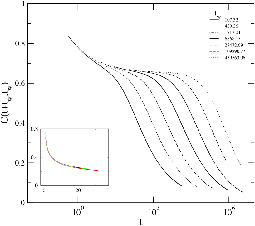
Figure 2: The correlation $C(t+t_{\mathrm{w}},t_{\mathrm{w}})$ vs. $t$ for a set of waiting times $t_{\mathrm{w}}$’s in the nonergodic phase, $a_{2}=0.5$ and $a_{3}=6.0$. Inset shows scaling of different $C(t+t_{\mathrm{w}},t_{\mathrm{w}})$’s as a function of $h(t+t_{\mathrm{w}})/h(t_{\mathrm{w}})$. Here $h(t)\equiv\exp[t^{1-\kappa}/(1-\kappa)]$ with $\kappa=.96$.

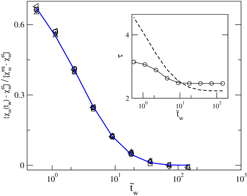
Figure 3: Scaled function $(\chi_{\omega}(\tilde{t}_{\mathrm{w}})-\chi_{\omega}^{st})/(\chi_{\omega}^{eq}-\chi_{\omega}^{st})$ vs. $\tilde{t}_{\mathrm{w}}$. Different symbols represent data for different frequencies $\omega$. Solid line is a fit to modified KWW form with $\tau(\tilde{t}_{\mathrm{w}})$ and $\beta=0.55$. Inset shows the variation of the $\tau$ with $\tilde{t}_{\mathrm{w}}$, following the scheme of (a) Ref.(sengupta, ) (solid) and (b) Ref.(loidl, ) (dashed).

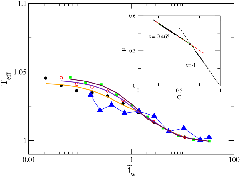
Figure 4: Effective temperature $T_{\mathrm{eff}}$ (see text) vs. waiting times $\tilde{t}_{\mathrm{w}}$ for $\omega=10^{-5}$(filled circle),$3\times 10^{-4}$(open circle), and $5\times 10^{-4}$ (filled square) in units of . Solid line corresponds to best fit curve of theoretical results. Experimental data of Ref. (israloff, ) shown with filled triangles. Inset shows $-F(t+t_{\mathrm{w}},t_{\mathrm{w}})$ vs. $C(t+t_{\mathrm{w}}),t_{\mathrm{w}})$ corresponding to the data of fig. 2. The slope in the FDT violation regime is $m=0.465$.

References

- (1) M. D. Ediger, C. A. Angell, and S. R. Nagel, J. Phys. Chem., 10 13200, (1999).
- (2) L. C. E. Struik , Physical Aging in Amorphous Polymers and Other Materials, Elsevier, (1978).
- (3) T. R. Kirkpatrick and D. Thirumalai Phys. Rev. B 36, 5388 (1987).
- (4) S. P. Das , Rev. of Mod. Phys., 76, 785, 2004.
- (5) L. F. Cugliandolo and J. Kurchan , Phys. Rev. Lett., 71, 173 (1993).
- (6) J. P. Bouchaud, J. Phys. (Paris) 2, 1705 (1992).
- (7) A. Crisanti and H.-J. Sommers, Z. Phys. B 87, 341 (1992).
- (8) R. Kühn and U. Horstmann, Phys. Rev. Lett., 78, 4067 (1997); R. Kühn, Europhys. Lett., 62, 313 (2003).
- (9) L. Lukenhemier R. Wehn U. Schneider and A. Loidl, Phys. Rev. Lett. 95, 055702 (2005).
- (10) P.C. Martin, E.D. Siggia and H.A. Rose, Phys. Rev. A 8, 423 (1973); R. V. Jensen, J. Stat. Phys. 25 183 (1981).
- (11) W. Gőtze, and L. Sjőgren, Rep. Prog. Phys. 55, 241 (1992).
- (12) B. Kim and G. F. Mazenko , Phys. Rev. A 45, 2393 (1992).
- (13) L. Berthier G. Biroli, J.-P. Bouchaud W. Kob K. Miyazaki and D. R. Reichman, J. Chem. Phys. 126, 184504 (2007).
- (14) B. Kim and A. Latz , Europhys. Lett., 53, 660 (2001).
- (15) E. Vincent and J. Hammann and M. Ocio, J-P Bouchaud and L. F. Cugliandolo , Proceedings of the XIV Sitges Conference Barcelona, 1996.
- (16) B. Sengupta and S. P. Das , Phys. Rev. E, 75, 061502 (2007).
- (17) T. S. Grigera and N. E. Israeloff, Phys. Rev. Lett. 83, 5038 (1999).
- (18) W. Kob and J. L. Barrat , Phys. Rev. Lett. 79, 360 (1979).
- (19) Sunil P. Singh and Shankar P. Das, unpublished.