Excitations of attractive 1-D bosons: Binding vs. fermionization

Abstract

The stationary states of few bosons in a one-dimensional harmonic trap are investigated throughout the crossover from weak to strongly attractive interactions. For sufficient attraction, three different classes of states emerge: (i) $N$-body bound states, (ii) bound states of smaller fragments, and (iii) gas-like states that fermionize, that is, map to ideal fermions in the limit of infinite attraction. The two-body correlations and momentum spectra characteristic of the three classes are discussed, and the results are illustrated using the soluble two-particle model.

I Introduction

In recent years, ultracold atoms have become a flexible tool for the simulation of fundamental quantum systems pethick ; pitaevskii ; bloch07 . Their versatility derives mainly from the fact that both their external forces and atomic interactions can be designed to a great extent. One striking example is the possibility to confine the atoms’ motion to lower dimensions, such as in the one-dimensional (1D) Bose gas bloch07 . Since, pictorially speaking, particles moving on a line cannot move around each other, they are in a sense more strongly correlated than their higher-dimensional counterparts. Moreover, their effective interaction strength can be tuned freely so as to enter the interesting regime of strong interactions, either via Feshbach resonances of the 3D scattering length koehler06 or through confinement-induced resonances of the effective 1D coupling Olshanii1998a .

The case of repulsive interactions has long received considerable attention, mostly for the striking feature that, in the hard-core limit of infinite repulsion between the bosons, the system maps to an ideal Fermi gas girardeau60 . In this fermionization limit, the bosons become impenetrable, which has a similar effect as Pauli’s exclusion principle for identical fermions. The seminal exact solutions derived for special systems at arbitrary interaction strength—such as the homogeneous Bose gas on a ring in the thermodynamic limit lieb63a ; lieb63b as well as for definite particle numbers sakmann05 , and for the inhomogeneous gas in a hard-wall trap hao06 —have recovered this borderline case in the limit of infinite coupling. The thermodynamic nature of the fermionization crossover from weak to strong repulsion has first been explored and contrasted with the complementary Thomas-Fermi regime petrov00 ; dunjko01 , and its microscopic mechanism has been unraveled by recent numerically exact studies deuretzbacher06 ; zoellner06a ; zoellner06b ; schmidt07 . Moreover, its experimental demonstration has sparked renewed interest in 1D bosons kinoshita04 ; paredes04 .

By contrast, the understanding of the attractive case is more patchy. In the homogeneous system, the ground state forms an $N$-body bound state mcguire64 . For sufficient attraction, it becomes ever more localized and is unstable in the thermodynamic limit. For finite systems, though, the ground state remains stable for arbitrary finite attraction, as is demonstrated by the exact solution via Bethe’s ansatz for a ring sakmann05 and a hard-wall trap hao06 . Much less is known about excited states. In the homogeneous system again, Monte Carlo simulations have indicated the existence of a highly excited gas-like state for ultrastrong attraction, which can be seen as the counterpart of the fermionized ground state for repulsive interactions astrakharchik05 ; astrakharchik04a . The evidence for this super-Tonks gas has been supported by a Bethe-ansatz solution batchelor05 . Still, an intuitive understanding of these states from a microscopic perspective and how they come about in the crossover from weak interactions is still missing. The complementary crossover for the low-lying excitation spectrum in turn has been investigated recently for the homogeneous system sykes07 ; however, it does not include the gas-like super-Tonks gas.

In this article, we study the entire crossover from the non-interacting to the strongly attractive limit for few bosons in a harmonic trap. This is done via the numerically exact multi-configuration time-dependent Hartree method introduced in Sec. II. Section III presents the general Bose-Fermi map valid for the gas-like super-Tonks states, and illustrates its meaning on the simple model of two bosons. The numerical investigation of the stationary states in Sec. IV reveals three distinct classes for strong enough attraction: $N$-body bound states (Sec. IV.1), states involving smaller fragments (Sec. IV.2), and finally gas-like states that fermionize (Sec. IV.3).

II Model and computational method

Model

We consider $N$ trapped bosons described by the Hamiltonian

$$H=\sum_{i=1}^{N}\left[\frac{1}{2}p_{i}^{2}+U(x_{i})\right]+g\sum_{i<j}\delta_{\sigma}(x_{i}-x_{j}).$$

We will focus on the case of harmonic confinement, $U(x)=\frac{1}{2}x^{2}$ (where harmonic-oscillator units are employed throughout.) The effective interaction resembles a 1D contact potential, but is mollified with a Gaussian $\delta_{\sigma}(x)\equiv e^{-x^{2}/2\sigma^{2}}/\sqrt{2\pi}\sigma$ (of width $\sigma=0.05$) for numerical reasons (cf. zoellner06a for details.) We concentrate on attractive forces $g\in(-\infty,0]$, which can be achieved experimentally by either having negative scattering lengths or by reducing the transverse confinement length $a_{\perp}\equiv\sqrt{\hbar/M\omega_{\perp}}$ sufficiently Olshanii1998a .

Computational method

Our approach relies on the numerically exact multi-configuration time-dependent Hartree method mey90:73 ; bec00:1 ; mctdh:package , a quantum-dynamics approach which has been applied successfully to systems of few identical bosons zoellner06a ; zoellner06b ; zoellner07a ; zoellner07c ; zoellner07b as well as to Bose-Bose mixtures zoellner08b . Its principal idea is to solve the time-dependent Schrödinger equation $\begin{array}[]{c}i\dot{\Psi}(t)=H\Psi(t)\end{array}$ as an initial-value problem by expanding the solution in terms of direct (or Hartree) products $\Phi_{J}\equiv\varphi_{j_{1}}\otimes\cdots\otimes\varphi_{j_{N}}$:

$$\Psi(t)=\sum_{J}A_{J}(t)\Phi_{J}(t).$$ (1)

The unknown single-particle functions $\varphi_{j}$ ($j=1,\dots,n$) are in turn represented in a fixed basis of, in our case, harmonic-oscillator orbitals. The permutation symmetry of $\Psi$ is ensured by the correct symmetrization of the expansion coefficients $A_{J}$.

Note that, in the above expansion, not only the coefficients $A_{J}$ but also the single-particle functions $\varphi_{j}$ are time dependent. Using the Dirac-Frenkel variational principle, one can derive equations of motion for both $A_{J},\varphi_{j}$ bec00:1 . Integrating this differential-equation system allows us to obtain the time evolution of the system via (1). This has the advantage that the basis set $\{\Phi_{J}(t)\}$ is variationally optimal at each time $t$; thus it can be kept relatively small.

Although designed for time-dependent studies, it is also possible to apply this approach to stationary states. This is done via the so-called relaxation method kos86:223 . The key idea is to propagate some wave function $\Psi(0)$ by the non-unitary $e^{-H\tau}$ (propagation in imaginary time.) As $\tau\to\infty$, this exponentially damps out any contribution but that stemming from the true ground state like $e^{-(E_{m}-E_{0})\tau}$. In practice, one relies on a more sophisticated scheme termed improved relaxation mey03:251 ; meyer06 , which is much more robust especially for excitations. Here $\langle\Psi|H|\Psi\rangle$ is minimized with respect to both the coefficients $A_{J}$ and the orbitals $\varphi_{j}$. The effective eigenvalue problems thus obtained are then solved iteratively by first solving for $A_{J}$ with fixed orbitals and then ‘optimizing’ $\varphi_{j}$ by propagating them in imaginary time over a short period. That cycle will then be repeated.

III Bose-Fermi map for attractive bosons

In this section, we state the general Bose-Fermi map and discuss its application to infinitely attractive interactions. (Without loss of generality, we focus on the time-independent formulation.) Its intuitive meaning will be illustrated on the special example of two harmonically trapped bosons.

III.1 General map

The Schrödinger equation of $N$ bosons with point interactions, $(E-H)\Psi=0$, is equivalent to a noninteracting system $(E-H_{0})\Psi=0$ with boundary conditions

$$2\left.\partial_{r}\Psi\right|_{r=0^{+}}=\left.g\Psi\right|_{r=0},$$ (2)

where $r\equiv x_{i}-x_{j}$ for fixed $i\neq j$. For infinitely repulsive interactions, $g\to\infty$, the constraint that

$$\left.\frac{\partial_{r}\Psi}{\Psi}\right|_{r=0^{+}}\to+\infty$$

leads to the well-known hard-core boundary conditions

$$\left.\Psi\right|_{x_{i}=x_{j}}=0,\qquad i\neq j.$$ (3)

Since, otherwise, $\Psi$ fulfills the noninteracting Schrödinger equation, it is intelligible that it can be mapped to a noninteracting state $\Psi_{-}$ of identical fermions, which automatically satisfies the hard-core boundary condition (3) by Pauli’s exclusion principle girardeau60 :

$$\Psi=A\Psi_{-},\quad A(X)\equiv\prod_{i<j}\mathrm{sgn}(x_{i}-x_{j}).$$

The Bose-Fermi map $A$ serves only to restore bosonic permutation symmetry. Note that, since $A^{2}=1$, all local quantities derived from $\rho_{N}=\left|\Psi\right|^{2}$ will coincide with those computed from the fermion state. In this sense, the case of infinite repulsion is commonly referred to as fermionization limit (“Tonks gas”).

By contrast, the constraint for infinite attraction

$$\left.\frac{\partial_{r}\Psi}{\Psi}\right|_{r=0^{+}}\to-\infty$$

may be satisfied by (a) $\left.\partial_{r}\Psi\right|_{0^{+}}\to-\infty$ (provided $\left.\Psi\right|_{0}>0$ diverges more slowly than the local derivative) or (b) $\left.\Psi\right|_{0}\to 0^{-}$ (assuming $\left.\partial_{r}\Psi\right|_{0^{+}}>0$) . If case (b) applies to all $i\neq j$, then we recover the hard-core gas above. Consequently, the Bose-Fermi mapping $\Psi=A\Psi_{-}$ then holds for $g\to-\infty$ as well. In particular, the energetically lowest such state exactly equals the fermionized repulsive ground state – the Tonks gas. However, for strong attraction, this eigenstate will be highly excited, whereas the ground state will be strongly bound. For finite $g>-\infty$, this may be identified with the super-Tonks state in Ref. astrakharchik05 .

A few comments are in order:

(i) By construction, this holds for any external potential $U$, just like the standard Bose-Fermi map. In particular, the analytic solution for $N$ bosons in a harmonic trap carries right over girardeau01

$$\Psi\left(X\right)\propto e^{-|X|^{2}/2}\negthickspace\prod_{1\leq i<j\leq N}\negthickspace|x_{i}-x_{j}|,$$ (4)

and likewise for the homogeneous system girardeau60 .

(ii) By the same logic as above, this extends to binary mixtures of bosons (for the repulsive case, cf. girardeau07 ). Likewise, the generalized Bose-Fermi map for spinor bosons deuretzbacher08 ought to apply also to the limit of infinite attraction.

(iii) The map also holds in the presence of additional long-range interactions, such as in dipolar gases astrakharchik08 .

III.2 Illustration

To visualize the above argument, let us resort to the simple model of two bosons in a harmonic-oscillator (HO) potential, $U(x)=\frac{1}{2}x^{2}$. Here the center of mass (CM) $R=\frac{1}{N}\sum_{i}x_{i}$ and the relative coordinate $r=x_{1}-x_{2}$ separate,

$$H=h_{\mathrm{CM}}+H_{\mathrm{rel}}\equiv\left[\frac{p_{R}^{2}}{2N}+\frac{1}{2}NR^{2}\right]+\left[p_{r}^{2}+\frac{1}{4}r^{2}+g\delta(r)\right]\!.$$

One can therefore write the wave function and its energy as

$$\Psi=\phi_{\mathcal{N}}\otimes\psi;\quad E=(\mathcal{N}+{\scriptstyle\frac{1}{2}})+\epsilon_{\mathrm{}},$$

where $\phi_{\mathcal{N}}$ is the HO orbital with quantum number $\mathcal{N}=0,1,\dots$ . The relative Hamiltonian may be viewed as a harmonic potential split into halves in the center, i.e., at the point of collision $r=0$. There the delta function imposes the boundary condition (2), which amounts to a cusp for $g<0$. The problem can be solved analytically in terms of parabolic cylinder functions $U(a,b)$ Busch98 ; cirone01

$$\psi_{\epsilon}(r)=cU(-\epsilon,r),$$ (5)

where $\epsilon(g)\equiv\nu(g)+\frac{1}{2}$ is determined through the transcendental equation

$$\nu(g)\in f_{g}^{-1}(0):\quad f_{g}(\nu):=2^{3/2}\frac{\Gamma\left(\frac{1-\nu}{2}\right)}{\Gamma\left(-\frac{\nu}{2}\right)}+g.$$ (6)

The solution for attractive interactions is plotted in Fig. 1:

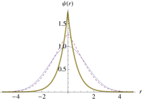
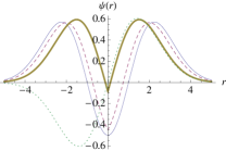
Figure 1: (color online) Relative wave function $\psi_{\nu(g)}(r)$ of two bosons in a harmonic trap (in arbitrary units).
(a) Ground state for attractive interactions: The Gaussian ground state ($\nu(g=0)=0$, thin-blue line) becomes peaked for $g=-0.6$ (dashed-magenta). This tends to an exponential peak as $g\to-\infty$ (cf. $g=-3.2$, thick-ocher line).
(b) Excited states for attractive interactions: The first bosonic excitation ($\nu=2$, thin-blue line) picks up a cusp at zero for $g=-1.5$ (dashed-magenta). As $g\to-\infty$ (cf. $g=-16$, thick-ocher), this cusp becomes sharper but, at the same time, is damped out more and more until the wave function’s modulus equals the fermionic state $u_{1}(r)\propto r\,e^{-r^{2}/4}$ (dotted-green).

• First imagine we start from the noninteracting ground state $\nu(0)=0$ (Fig. 1a). For $g<0$, the Gaussian will pick up a cusp at $r=0$, which becomes ever sharper for increasing $\left|g\right|$, i.e., $\psi^{\prime}(0^{+})\to-\infty$. In the limit $g\to-\infty$, when the support of $\psi$ becomes much smaller than the oscillator length, this is described simply by the bound state of the delta potential, $\psi(r)\sim\frac{1}{\sqrt{a}}e^{-\left|r\right|/a}$ with $a\equiv-2/g$ the 1D scattering length. Clearly $\left|\psi(r)\right|^{2}\stackrel{{\scriptstyle g\to-\infty}}{{\to}}$$\delta(r)$.

• An eigenstate with $\nu(0)=2n\neq 0$ will also form a cusp at $r=0$ (Fig. 1b). In contrast to before, however, this peak will become ever smaller for $g\to-\infty$, until it reaches down to $\psi(0)=0$ for infinite attraction. In this limit, the wave function’s modulus equals that of the next lower fermionic state, $\psi(r)\to\mathrm{sgn}(r)u_{2n-1}(r)$, where $u_{a}(r)\propto H_{a}\left(\frac{r}{\sqrt{2}}\right)\,e^{-r^{2}/4}$. Concomitantly, the energy will be lowered to $\lim_{g\to-\infty}\nu(g)=2n-1$, which matches exactly the fermionized level $\lim_{g\to+\infty}\bar{\nu}(g)$ starting from $\bar{\nu}(0)=2(n-1)$.

IV Molecule formation vs. fermionization in a harmonic trap

After having presented the general mapping valid for infinite attraction, let us now investigate the crossover to that borderline case, starting from the noninteracting states. For concreteness, we shall focus on the case of $N=3$ bosons in a harmonic trap.

Figure 2: Energy spectrum $\{E_{m}(g)\}$ of $N=3$ bosons in a harmonic trap. Different line styles correspond to states which connect to a trimer (- - -), a dimer plus a single boson ($-\cdot-$), and a gas-like fermionized state (—), respectively. Inset: Energy $E(g)$ for the lowest fermionized states of $N=2-4$ atoms (bottom to top).

Figure 2 explores the evolution of the low-lying few-body spectrum $\{E_{m}(g)\}$ as we vary $g\leq 0$. In the absence of interactions, the spectrum exhibits an even spacing, which comes about by distributing all $N$ particles in number states $|\boldsymbol{N}\rangle=|N_{0},N_{1},\dots\rangle$ over the lowest HO levels $\epsilon_{a}=a+\frac{1}{2}$. Clearly, Fig. 2 reveals that, when attractive interactions $g<0$ are switched on, the depicted spectrum falls apart into three (for $N=3$) qualitatively different subclasses. In anticipation of our analysis below, we identify the asymptotically lowest set of levels as $N$-body bound states (or trimers), the cluster on top of these as hybrid states (dimers plus one free boson), and the highest level as gas-like state which undergoes fermionization. Note that, by CM separation, for each state there is a countable set of copies with different CM energies $\mathcal{N}+\frac{1}{2}$, which are shifted with respect to one another.

IV.1 Trimer states

Figure 3: One-body density $\rho(x)$ for the ground state (a), some hybrid state (b), and the lowest fermionizing state (c) of $N=3$ bosons, plotted for different interaction strengths $g$.

The ground state, as well as its copies with higher CM excitations, can be thought of as an $N$-body bound state, which would be the straightforward generalization of the two-body bound state discussed in Sec. III.2. In fact, this class of states is well known from the homogeneous system mcguire64 , where an analytic solution is available via Bethe’s ansatz sakmann05 ; sykes07

$$E(g)\propto-cg^{2}N(N^{2}-1);\quad\Psi(X)\propto e^{-\sum_{i<j}|x_{i}-x_{j}|/a},$$ (7)

where $a\equiv-2/g$ is the 1D scattering length. We will now argue that, for sufficient attraction, this wave function also holds in our case of harmonic confinement, up to a trivial CM factor $\phi_{\mathcal{N}}$. To this end, let us proceed like in mcguire64 and transform $X\equiv(x_{1},\dots,x_{N})^{\top}$ to Jacobian coordinates $Y\equiv(R,r_{1},,\dots,r_{N-1})^{\top}$, here for simplicity specified for $N=3$:

$$Y=\mathcal{O}X,\;\mathcal{O}=\left(\begin{array}[]{ccc}\frac{1}{\sqrt{3}}&\frac{1}{\sqrt{3}}&\frac{1}{\sqrt{3}}\\ \frac{1}{\sqrt{2}}&\frac{-1}{\sqrt{2}}&0\\ \sqrt{\frac{2}{3}}\frac{1}{2}&\sqrt{\frac{2}{3}}\frac{1}{2}&-\sqrt{\frac{2}{3}}\end{array}\right).$$

Up to a factor, $R$ ($r_{1}$) coincide with the usual center of mass (two-particle relative coordinate), while $r_{2}$ gives the difference between particle $\#3$ and the center of mass of the cluster $(1,2)$. By orthogonality of $\mathcal{O}$, the Hamiltonian transforms to $H(Y)=h_{CM}+H_{\mathrm{rel}}$, with

$$H_{\mathrm{rel}} = \sum_{k=1}^{2}\left[\frac{1}{2}p_{r,k}^{2}+\frac{1}{2}r_{k}^{2}\right]+$$

$$g\left\{\frac{1}{\sqrt{2}}\delta(r_{1})+\sqrt{2}\sum_{\pm}\delta(r_{1}\pm\sqrt{3}r_{2})\right\}.$$

If all $N$ particles cling together to form a tightly bound state, then their distances will be small compared to the confinement scale, $\left|r_{k}\right|\ll 1$. In this limit, $\frac{1}{2}r_{k}^{2}$ may be safely neglected, so that the relative wave function asymptotically maps to the homogeneous form (7). Likewise, the energy scales as $E(g)\sim\mathcal{N}+\frac{N}{2}-\alpha_{N}g^{2}$ ($\alpha_{N}>0$).

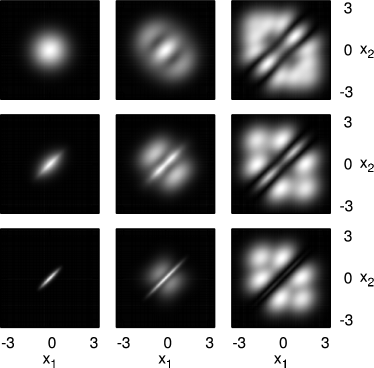
Figure 4: Two-body correlation functions $\rho_{2}(x_{1},x_{2})$ for the ground state, some hybrid state, and the lowest fermionizing state (from left to right), at coupling strengths $g=-0.1,\,-2$ and $-10$ (from top to bottom).

A look at the one-body density profiles $\rho(x)=\langle x|\rho_{1}|x\rangle$ shown in Fig. 3(a) confirms that this state becomes more and more localized. In contrast to the translation-invariant homogeneous case, this “soliton”-like state is localized even in the one-body density, which represents an average over all measurements. Moreover, in contrast to the hard-wall trap hao06 , there is no tipping point where the width $(\Delta x)^{2}=\langle x^{2}\rangle$ would become larger again and return to its noninteracting value for $g\to-\infty$. In fact, here $\Delta x$ decreases monotonically for $g\to-\infty$ and eventually saturates in the CM density

$$\lim_{g\to-\infty}\rho(x)=\left|\phi_{\mathcal{N}}(x)\right|^{2},$$ (9)

whose length scale $a_{\mathrm{CM}}=1/\sqrt{N}$ is suppressed by the total mass $NM$ (in units of the atomic mass $M\equiv 1$). To prove this, note that by CM separation,

$$\rho(x_{1})=\int\negmedspace dx_{2}\cdots dx_{N}\left|\phi_{\mathcal{N}}\left(R\right)\right|^{2}\negmedspace\rho_{\mathrm{rel}}(r\equiv\{r_{k}\}).$$

For increasing attraction, $\lim_{g\to-\infty}\rho_{\mathrm{rel}}(r)=\delta(r)$, in agreement with (7). Fig. 4 visualizes that the two-body density $\rho_{2}(x_{1},x_{2})=\langle x_{1},x_{2}|\rho_{2}|x_{1},x_{2}\rangle$ is more and more concentrated on the diagonal $\{x_{1}=x_{2}\}$. Carrying out the trivial integrals proves Eq. (9), which reflects that all atoms clump together to point-like molecule whose position coincides with the CM. (Of course, the validity of our effective model requires the molecule to be still large compared to the spatial extension of the atoms.)

That line of reasoning fails in the hard-wall trap, where $R$ and $r$ couple strongly due to the anharmonicity of $U(x)$ matthies07 ; in fact, for very tight binding of two particles, their common CM would be permitted to spread out over the whole box, thus compensating the stronger localization in the relative coordinate. A simple dimensional argument to see this is that the length scale in a hard-wall trap is simply the size of the box, independent of the object’s mass – in contrast to the harmonic oscillator.

IV.2 Hybrid states

The behavior of the class of levels on top of the trimer levels ($N=3$, Fig. 2) is clearly more complex, which indicates that different CM excitations $\mathcal{N}$ are involved. On the one hand, the levels are significantly above those of the $N$-body bound states; on the other hand, they do not saturate with increasing attraction. This suggests to identify these three-boson states with the formation of dimers plus one unbound atom. For general $N$, this class of hybrid states involves different fragments—labeled $f=1,\dots,F$—of $N_{f}$-body bound states, where $\sum_{f=1}^{F}N_{f}=N$ and $F=2,\dots,N-1$.

Figure 3(b) shows the density profile of the lowest hybrid state, which has $\mathcal{N}=0$. A pronounced peak at $x=0$ builds up similar to the trimer case, but with a non-Gaussian structure indicative of relative excitations. This becomes clearer from a look at the two-body density in Fig. 4: For increasing attraction, part of the bosons clump together, as is visible from the “molecule” peak at $\{x_{1}=x_{2}\}$. However, unlike before, a non-negligible part remains isolated at $\{x_{1}=-x_{2}\}$. To understand this pattern a little better, let us revisit the Hamiltonian (IV.1). If we assume that only two of the three bosons bind, say $\left|r_{1}\right|\ll 1$ (up to permutation symmetry $S_{+}$), then we end up with two decoupled Hamiltonians,

$$H_{\mathrm{rel}}\approx\!\left[\frac{1}{2}p_{r,1}^{2}+\frac{g}{\sqrt{2}}\delta(r_{1})\right]+\left[\frac{1}{2}p_{r,2}^{2}+\frac{1}{2}r_{2}^{2}+2\sqrt{\frac{2}{3}}g\delta(r_{2})\right]\!,$$

one for a free-space molecule ($r_{1}$, relating to the relative ground state described in Fig. 1a) and one for an effective particle in an excited state of an oscillator with a delta-type dimple at the origin ($r_{2}$, the lowest excitation corresponding to Fig. 1b). This yields the relative wave function (excluding the trivial CM factor)

$$\psi(X)\propto S_{+}\left\{e^{-|x_{1}-x_{2}|/a}U\left(-\epsilon,\frac{1}{2}(x_{1}+x_{2})-x_{3}\right)\right\},$$

where the parameters are determined in analogy to Eq. (5). We have checked that this expression qualitatively reproduces the two-body pattern in Fig. 4 for $g\to-\infty$. That makes it tempting to think of the hybrid state as a hard-core “gas” of a dimer—clumped near the trap center—and a third, unbound boson. In that regime, the energy scales as $E(g)\sim\mathcal{N}+\frac{N}{2}-\frac{1}{2a^{2}}+\alpha$, where $\lim_{g\to-\infty}\epsilon(g)-\frac{1}{2}\equiv\alpha\in 2\mathbb{N}-1$. In general, there can be different combinations of relative and CM excitations ($\mathcal{N}\neq 0$) which give nearly the same energy – this explains the splittings of all but the lowest hybrid levels in Fig. 2.

IV.3 Fermionizing states

Let us now focus on the highest level in Fig. 2, which is the energetically lowest gas-like state. Its energy does not diverge quadratically with $g\to-\infty$, but rather saturates. By the fermionization map above, its limit is simply the energy of $N$ free fermions, $\lim_{g\to-\infty}E(g)=\sum_{a=0}^{N-1}\epsilon_{a}=\frac{N^{2}}{2}$ (see Fig. 2, inset), and likewise for higher excitations. Evidently, this requires a huge energy for the connecting level $E(g=0)>E(-\infty)$ if $N\gg 1$. In fact, the difference between the two equals that between the noninteracting ground state $N\epsilon_{0}$ and its fermionization limit $\sum_{a=0}^{N-1}\epsilon_{a}$, which can be written down explicitly in a harmonic trap,

$$\left|E(g\to-\infty)-E(0)\right|=\frac{N^{2}}{2}-\frac{N}{2}=\frac{N(N-1)}{2}.$$

This can be thought of as increasing (lowering) the energy by $\Delta\epsilon=1$ for each pair $(i<j)$. Therefore, the “super-Tonks” level connects to the noninteracting level $E(0)=\frac{N^{2}}{2}+\frac{N(N-1)}{2}=N(N-\frac{1}{2})$, as may be verified for $N\leq 4$ in Fig. 2(inset).

Accordingly, the corresponding many-body state is expected to evolve to (4). A glimpse of this can be gotten from the density profile shown in Fig. 3(c), where the $N$ density wiggles characteristic of the Tonks gas emerge, $\rho=\sum_{a=0}^{N-1}|\phi_{a}|^{2}$ (a similar observation has been stated in Ref. astrakharchik04a ). In the repulsive case, this has the familiar interpretation that the $N$ bosons localize on $N$ more or less “discrete” spots due to a trade-off between mutual isolation and external confinement deuretzbacher06 ; zoellner06a .

Some more insight into this crossover is given by the two-body correlation function $\rho_{2}(x_{1},x_{2})$ (Fig. 4). As expected from the two-atom toy model (Sec. III.2), the diagonal $\{x_{1}=x_{2}\}$ “damps out” more and more. The fact that it persists even for couplings as large as $g=-10$ underscores the notion of the (finite-$g$) super-Tonks gas being more strongly correlated than its repulsive counterpart astrakharchik05 . This in turn relates to the picture that, due to a positive 1D scattering length $a=-2/g$, a small region is excluded from the scattering zone, so that the hard core effectively extends to a nonzero volume. This also offers an explanation for another phenomenon: As $g\to-\infty$, we see that the typical fermionized checkerboard pattern forms in the two-body density girardeau01 ; zoellner06b . This signifies that, upon measuring a first boson at, say, $x_{1}\approx 0$, the remaining $N-1=2$ bosons are pinpointed to discrete positions $x_{2}\approx\pm 1.5$. However, here the peaks are much more pronounced than in the Tonks gas, which may be accounted for by a “thicker” hard core between the atoms.

Figure 5: Momentum distribution $\tilde{\rho}(k)$ for the ground state (a), the lowest hybrid state (b), and the lowest fermionizing state (c) of $N=3$ bosons, plotted for different interaction strengths $g$.

We have so far looked into local observables, where the fermionization limit imprints truly fermionic properties on the bosons. By contrast, nonlocal features as evidenced, e.g., in the experimentally relevant momentum distribution

$$\tilde{\rho}(k)=2\pi\langle k|\rho_{1}|k\rangle=\int dx\int dx^{\prime}e^{-ik(x-x^{\prime})}\rho_{1}(x,x^{\prime})$$

reflect nontrivial differences from the ideal Fermi gas. Figure 5(c) shows the evolution of $\tilde{\rho}(k)$ for the gas-like state in juxtaposition with the trimer and dimer states [Figs. 5(a-b)]. For the ground state, where all bosons simply form an ever tighter $N$-body molecule as $g\to-\infty$, $\rho_{1}(x,x^{\prime})\propto\delta(x-x^{\prime})$ loses all long-range order, i.e., $\rho_{1}(x,x^{\prime})=0$ for $|x-x^{\prime}|>0$. By complementarity, its momentum spectrum trivially approaches a flat shape. Things are more complicated for the hybrid state in Fig. 5(b): Since only two bosons bind and, as a whole, form a hard-core composite with the remaining atom, some long-range order is preserved, so that the central peak $\tilde{\rho}(0)$ persists even for large values of $|g|$. Note that, as in the repulsive case, the hard-core short-range correlations enforce an algebraic decay for high momenta, $\tilde{\rho}(k)\sim c/k^{4}$ minguzzi02 . Finally, the gas-like state exhibits the most interesting behavior (Fig. 5c). The initially box-like distribution $\tilde{\rho}(k)=2\pi\rho(k)$ (harmonic trap at $g=0$) forms a strong $k=0$ peak highly reminiscent of the Tonks gas deuretzbacher06 ; zoellner06b . Also note the slow formation of the characteristic $k^{-4}$ tails. This complements our picture of the crossover from zero to strongly attractive interactions.

V Summary

In this work, we have brought together the subjects of attractive, one-dimensional Bose gases—which currently are of great interest and experimentally relevant—and the binding properties of few-body systems. We have studied the stationary states of one-dimensional bosons in a harmonic trap throughout the crossover from weakly to strongly attractive interactions.

Three different classes of states have emerged for strong enough attraction: (i) The ground state and its center-of-mass excitations become $N$-body bound states, for which any two particles pair up to a tightly bound molecule. Its binding length $a$ shrinks to zero with increasing attraction, and thus the relative motion becomes independent of the trap geometry. (ii) By contrast, certain highly excited states fermionize, i.e., they map to an ideal Fermi state for infinite attraction. Both the typical fermionic density profile with $N$ maxima and, more generally, the characteristic checkerboard pattern in the two-body density have been evidenced, signifying localization of the individual atoms. Also, the formation of a hard-core momentum distribution has been witnessed, with a zero-momentum peak and an algebraic decay for large momenta. (iii) Between these two extremes, there is a rich class of hybrid states featuring mixed molecule and hard-core boundary conditions. For the special case of $N=3$ atoms, this class consists of a dimer plus a single boson, with a hard-core separation between the two.

Even though we have focused mostly on few atoms ($N=3$) in a harmonic trap, these results reflect the microscopic mechanism for arbitrary atom numbers and external potentials.

- (1) C. J. Pethick and H. Smith, Bose-Einstein condensation in dilute gases (Cambridge University Press, Cambridge, 2001).
- (2) L. Pitaevskii and S. Stringari, Bose-Einstein Condensation (Oxford University Press, Oxford, 2003).
- (3) I. Bloch, J. Dalibard, and W. Zwerger, arXiv:0704.3011 .
- (4) T. Köhler, K. Góral, and P. S. Julienne, Rev. Mod. Phys. 78, 1311 (2006).
- (5) M. Olshanii, Phys. Rev. Lett. 81, 938 (1998).
- (6) M. Girardeau, J. Math. Phys. 1, 516 (1960).
- (7) E. H. Lieb and W. Liniger, Phys. Rev. 130, 1605 (1963).
- (8) E. H. Lieb, Phys. Rev. 130, 1616 (1963).
- (9) K. Sakmann, A. I. Streltsov, O. E. Alon, and L. S. Cederbaum, Phys. Rev. A 72, 033613 (2005).
- (10) Y. Hao, Y. Zhang, J. Q. Liang, and S. Chen, Phys. Rev. A 73, 063617 (2006).
- (11) D. S. Petrov, G. V. Shlyapnikov, and J. T. M. Walraven, Phys. Rev. Lett. 85, 3745 (2000).
- (12) V. Dunjko, V. Lorent, and M. Olshanii, Phys. Rev. Lett. 86, 5413 (2001).
- (13) F. Deuretzbacher, K. Bongs, K. Sengstock, and D. Pfannkuche, Phys. Rev. A 75, 013614 (2007).
- (14) S. Zöllner, H.-D. Meyer, and P. Schmelcher, Phys. Rev. A 74, 053612 (2006).
- (15) S. Zöllner, H.-D. Meyer, and P. Schmelcher, Phys. Rev. A 74, 063611 (2006).
- (16) B. Schmidt and M. Fleischhauer, Phys. Rev. A 75, 021601 (2007).
- (17) T. Kinoshita, T. Wenger, and D. S. Weiss, Science 305, 1125 (2004).
- (18) B. Paredes et al., Nature 429, 277 (2004).
- (19) J. B. McGuire, J. Math. Phys. 5, 622 (1964).
- (20) G. E. Astrakharchik, J. Boronat, J. Casulleras, and S. Giorgini, Phys. Rev. Lett. 95, 190407 (2005).
- (21) G. E. Astrakharchik, D. Blume, S. Giorgini, and B. E. Granger, J. Phys. B 37, S205 (2004).
- (22) M. T. Batchelor, M. Bortz, X. W. Guan, and N. Oelkers, J. Stat. Mech. 2005, L10001 (2005).
- (23) A. G. Sykes, P. D. Drummond, and M. J. Davis, Phys. Rev. A 76, 063620 (2007).
- (24) H.-D. Meyer, U. Manthe, and L. S. Cederbaum, Chem. Phys. Lett. 165, 73 (1990).
- (25) M. H. Beck, A. Jäckle, G. A. Worth, and H.-D. Meyer, Phys. Rep. 324, 1 (2000).
- (26) G. A. Worth, M. H. Beck, A. Jäckle, and H.-D. Meyer, The MCTDH Package, Version 8.2, (2000). H.-D. Meyer, Version 8.3 (2002). See http://www.pci.uni-heidelberg.de/tc/usr/mctdh/.
- (27) S. Zöllner, H.-D. Meyer, and P. Schmelcher, Phys. Rev. A 75, 043608 (2007).
- (28) S. Zöllner, H.-D. Meyer, and P. Schmelcher, Phys. Rev. Lett. 100, 040401 (2008).
- (29) S. Zöllner, H.-D. Meyer, and P. Schmelcher, arXiv:0801.1090v1 .
- (30) S. Zöllner, H.-D. Meyer, and P. Schmelcher, arXiv:0805.0738v1 .
- (31) R. Kosloff and H. Tal-Ezer, Chem. Phys. Lett. 127, 223 (1986).
- (32) H.-D. Meyer and G. A. Worth, Theor. Chem. Acc. 109, 251 (2003).
- (33) H.-D. Meyer, F. L. Quéré, C. Léonard, and F. Gatti, Chem. Phys. 329, 179 (2006).
- (34) M. D. Girardeau, E. M. Wright, and J. M. Triscari, Phys. Rev. A 63, 033601 (2001).
- (35) M. D. Girardeau and A. Minguzzi, Phys. Rev. Lett. 99, 230402 (2007).
- (36) F. Deuretzbacher et al., Phys. Rev. Lett. 100, 160405 (2008).
- (37) G. E. Astrakharchik and Y. E. Lozovik, Phys. Rev. A 77, 013404 (2008).
- (38) T. Busch, B. G. Englert, K. Rzazewski, and M. Wilkens, Found. Phys. 28, 549 (1998).
- (39) M. A. Cirone, K. Góral, K. Rzazewski, and M. Wilkens, J. Phys. B 34, 4571 (2001).
- (40) C. Matthies, S. Zöllner, H.-D. Meyer, and P. Schmelcher, Phys. Rev. A 76, 023602 (2007).
- (41) A. Minguzzi, P. Vignolo, and M. P. Tosi, Phys. Lett. A 294, 222 (2002).