Significant Diagnostic Counterexamples in Probabilistic Model Checking

Abstract

This paper presents a novel technique for counterexample generation in probabilistic model checking of Markov Chains and Markov Decision Processes. (Finite) paths in counterexamples are grouped together in witnesses that are likely to provide similar debugging information to the user. We list five properties that witnesses should satisfy in order to be useful as debugging aid: similarity, accuracy, originality, significance, and finiteness. Our witnesses contain paths that behave similar outside strongly connected components.

This papers shows how to compute these witnesses by reducing the problem of generating counterexamples for general properties over Markov Decision Processes, in several steps, to the easy problem of generating counterexamples for reachability properties over acyclic Markov Chains.

1 Introduction

Model checking is an automated technique that, given a finite-state model of a system and a property stated in an appropriate logical formalism, systematically checks the validity of this property. Model checking is a general approach and is applied in areas like hardware verification and software engineering.

Nowadays, the interaction geometry of distributed systems and network protocols calls for probabilistic, or more generally, quantitative estimates of, e.g., performance and cost measures. Randomized algorithms are increasingly utilized to achieve high performance at the cost of obtaining correct answers only with high probability. For all this, there is a wide range of models and applications in computer science requiring quantitative analysis. Probabilistic model checking allow us to check whether or not a probabilistic property is satisfied in a given model, e.g., “Is every message sent successfully received with probability greater or equal than $0.99$?”.

A major strength of model checking is the possibility of generating diagnostic information in case the property is violated. This diagnostic information is provided through a counterexample showing an execution of the model that invalidates the property under verification. Apart from the immediate feedback in model checking, counterexamples are also used in abstraction-refinement techniques [CGJ⁺00], and provide the foundations for schedule derivation (see, e.g., [BLR05]).

Although counterexample generation was studied from the very beginning in most model checking techniques, this has not been the case for probabilistic model checking. Only recently attention was drawn to this subject [AHL05, AL06, HK07a, HK07b, AL07], fifteen years after the first studies on probabilistic model checking. Contrarily to other model checking techniques, counterexamples in this setting are not given by a single execution path. Instead, they are sets of executions of the system satisfying a certain undesired property whose probability mass is higher than a given bound. Since counterexamples are used as a diagnostic tool, previous works on counterexamples have presented them as sets of finite paths of large enough probability. We refer to these sets as representative counterexamples. Elements of representative counterexamples with high probability have been considered the most informative since they contribute mostly to the property refutation.

A challenge in counterexample generation for probabilistic model checking is that (1) representative counterexamples are very large (often infinite), (2) many of its elements have very low probability, and (3) that elements can be extremely similar to each other (consequently providing similar diagnostic information). Even worse, (4) sometimes the finite paths with highest probability do not indicate the most likely violation of the property under consideration.

For example, look at the Markov chain $\operatorname{{\cal M}}$ in Figure 2. The property $\smash{{\operatorname{{\cal M}}}\models_{{}_{{}_{{\!\!\leq 0.5}}}}{\lozenge{\psi}}}$ stating that execution reaches a state satisfying $\psi$ (i.e., reaches $s_{3}$ or $s_{4}$) with probability lower or equal than $0.5$ is violated (since the probability of reaching $\psi$ is 1). The left hand side of table in Figure 2 lists finite paths reaching $\psi$ ranked according to their probability. Note that finite paths with highest probability take the left branch in the system, whereas the right branch in itself has higher probability, illustrating Problem 4. To adjust the model so that it does satisfy the property (bug fixing), it is not sufficient to modify the left hand side of the system alone; no matter how one changes the left hand side, the probability of reaching $\psi$ remains at least $0.6$. Furthermore, the first six finite paths provide similar diagnostic information: they just make extra loops in $s_{1}$. This is an example of Problem 3. Also, the probability of every single finite path is far below the bound $0.5$, making it unclear if a particular path is important; see Problem 2 above. Finally, the (unique) counterexample for the property $\smash{{\operatorname{{\cal M}}}\models_{{}_{{}_{{\!\!<1}}}}{\lozenge{\psi}}}$ consists of infinitely many finite paths (namely all finite paths of $\operatorname{{\cal M}}$); see Problem 1.

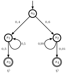
Figure 1: Markov chain

	Single paths		Witnesses
Rank	F. Path	Prob	Witness	Mass
1	$s_{0}(s_{1})^{1}s_{3}$	0.2	[$s_{0}s_{2}s_{4}$]	0.6
2	$s_{0}(s_{1})^{2}s_{3}$	0.1	[$s_{0}s_{1}s_{3}$]	0.4
3	$s_{0}(s_{1})^{3}s_{3}$	0.05
4	$s_{0}(s_{1})^{4}s_{3}$	0.025
5	$s_{0}(s_{1})^{5}s_{3}$	0.0125
6	$s_{0}(s_{1})^{6}s_{3}$	0.00625
7	$s_{0}(s_{2})^{1}s_{4}$	0.006
8	$s_{0}(s_{2})^{2}s_{4}$	0.0059
9	$s_{0}(s_{2})^{3}s_{4}$	0.0058
⋮	⋮	⋮

Figure 2:   Comparison Table

To overcome these problems, we partition a representative counterexample into sets of finite paths that follow a similar pattern. We call these sets witnesses. To ensure that witnesses provide valuable diagnostic information, we desire that the set of witnesses that form a counterexample satisfies several properties: two different witnesses should provide different diagnostic information (solving Problem 3) and elements of a single witness should provide similar diagnostic information, as a consequence witnesses have a high probability mass (solving Problems 2 and 4), and the number of witnesses of a representative counterexample should be finite (solving Problem 1).

In our setting, witnesses consist of paths that behave the same outside strongly connected components. In the example of Figure 2, there are two witnesses: the set of all finite paths going right, represented by [$s_{0}s_{2}s_{4}$] whose probability (mass) is $0.6$, and the set of all finite paths going left, represented by [$s_{0}s_{1}s_{3}$] with probability (mass) $0.4$.

In this paper, we show how to obtain such sets of witnesses for bounded probabilistic LTL properties on Markov decision processes ($\operatorname{MDP}$). In fact, we first show how to reduce this problem to finding witnesses for upper bounded probabilistic reachability properties on discrete time Markov chains ($\operatorname{MCs}$). The major technical matters lie on this last problem to which most of the paper is devoted.

In a nutshell, the process to find witnesses for the violation of $\smash{{\operatorname{{\cal M}}}\models_{{}_{{}_{{\!\!\leq p}}}}{\lozenge{\psi}}}$, with $\operatorname{{\cal M}}$ being a $\operatorname{MC}$, is as follows. We first eliminate from the original $\operatorname{MC}$ all the “uninteresting” parts. This proceeds as the first steps of the model checking process: make absorbing all state satisfying $\psi$, and all states that cannot reach $\psi$, obtaining a new $\operatorname{MC}$ $\operatorname{{\cal M}}_{\psi}$. Next reduce this last $\operatorname{MC}$ to an acyclic $\operatorname{MC}$ $\operatorname{Ac}(\operatorname{{\cal M}}_{\psi})$ in which all strongly connected components have been conveniently abstracted with a single probabilistic transition. The original and the acyclic $\operatorname{MC}$s are related by a mapping that, to each finite path in $\operatorname{Ac}(\operatorname{{\cal M}}_{\psi})$ (that we call rail), assigns a set of finite paths behaving similarly in $\operatorname{{\cal M}}$ (that we call torrent). This map preserves the probability of reaching $\psi$ and hence relates counterexamples in $\operatorname{Ac}(\operatorname{{\cal M}}_{\psi})$ to counterexamples in $\operatorname{{\cal M}}$. Finally, counterexamples in $\operatorname{Ac}(\operatorname{{\cal M}}_{\psi})$ are computed by reducing the problem to a $k$ shortest path problem, as in [HK07a]. Because $\operatorname{Ac}(\operatorname{{\cal M}}_{\psi})$ is acyclic, the complexity is lower than the corresponding problem in [HK07a].

It is worth to mention that our technique can also be applied to simple pCTL formulas without nested path quantifiers.

Organization of the paper.

Section 2 presents the necessary background on Markov chains ($\operatorname{MC}$), Markov Decision Processes ($\operatorname{MDP}$), and Linear Temporal Logic (LTL). Section 3 presents the definition of counterexamples and discuss the reduction from general LTL formulas to upper bounded probabilistic reachability properties, and the extraction of the maximizing $\operatorname{MC}$ in a $\operatorname{MDP}$. Section 4 discusses desire properties of counterexamples. In Sections 5 and 6, we introduce the fundamentals on rails and torrents, the reduction of the original $\operatorname{MC}$ to the acyclic one, and our notion of significant diagnostic counterexamples. Section 7 then present the techniques to actually compute counterexamples. In Section 8 we discuss related work and give final conclusions.

2 Preliminaries

2.1 Markov Decision Processes and Markov chains

Markov Decision Processes ($\operatorname{MDPs}$) constitute a formalism that combines nondeterministic and probabilistic choices. They are the dominant model in corporate finance, supply chain optimization, system verification and optimization. There are many slightly different variants of this formalism such as action-labeled $\operatorname{MDPs}$ [Bel57, FV97], probabilistic automata [SL95, SdV04]; we work with the state-labeled $\operatorname{MDPs}$ from [BdA95].

Definition 2.1.

Let $S$ be a set. A discrete probability distribution on $S$ is a function $p\colon S\to[0,1]$ with countable or finite carrier and such that $\sum_{s\in S}p(s)=1$. We denote the set of all discrete probability distributions on $S$ by $\operatorname{Distr}(S)$. Additionally, we define the Dirac distribution on an element $s\in S$ as $1_{s}$, i.e., $1_{s}(s)=1$ and $1_{s}(t)=0$ for all $t\in S\setminus\{s\}$.

Definition 2.2.

A Markov Decision Process ($\operatorname{MDP}$) is a four-tuple $\operatorname{{\cal D}}=(S,s_{0},L,\tau)$, where

• $S$ is the finite state space of the system;

• $s_{0}\in S$ is the initial state;

• $L$ is a labeling function that associates to each state $s\in S$ a set $L(s)$ of propositional variables that are valid in $s$;

• $\tau\colon S\to\wp(\operatorname{Distr}(S))$ is a function that associates to each $s\in S$ a non-empty and finite subset of $\operatorname{Distr}(S)$ of probability distributions.

Definition 2.3.

Let $\operatorname{{\cal D}}=(S,s_{0},\tau,L)$ be a $\operatorname{MDP}$. We define a successor relation $\delta\subseteq S\times S$ by $\delta\triangleq\{(s,t)|\exists\,\pi\in\tau(s)\;.\;\pi(t)>0\}$ and for each state $s\in S$ we define the sets

$$\operatorname{Paths}(\operatorname{{\cal D}},s)\triangleq\{s_{0}s_{1}s_{2}\ldots\in S^{\omega}|s_{0}=s\land\forall n\in\mathbb{N}\;.\;\delta(s_{n},s_{n+1})\}\mbox{ and}$$

$$\operatorname{Paths}^{\star}(\operatorname{{\cal D}},s)\triangleq\{s_{0}s_{1}\ldots s_{n}\in S^{\star}|s_{0}=s\land\forall\,0\leq i<n\;.\;\delta(s_{n},s_{n+1})\}$$

of paths and finite paths respectively beginning at $s$. We usually omit $\operatorname{{\cal D}}$ from the notation; we also abbreviate $\operatorname{Paths}(\operatorname{{\cal D}},s_{0})$ as $\operatorname{Paths}(\operatorname{{\cal D}})$ and $\operatorname{Paths}^{\star}(\operatorname{{\cal D}},s_{0})$ as $\operatorname{Paths}^{\star}(\operatorname{{\cal D}})$. For $\omega\in\operatorname{Paths}(s)$, we write the $(n\!+\!1)$-st state of $\omega$ as $\omega_{n}$. As usual, we let ${\cal B}_{s}\subseteq\wp(\operatorname{Paths}(s))$ be the Borel $\sigma$-algebra on the cones $\langle{s_{0}\dots s_{n}}\rangle\triangleq\{\omega\in\operatorname{Paths}(s)|\omega_{0}=s_{0}\land\ldots\land\omega_{n}=s_{n}\}$. Additionally, for a set of finite paths $\Lambda\subseteq\operatorname{Paths}^{\star}(s)$, we define $\langle{\Lambda}\rangle\triangleq\bigcup_{\sigma\in\Lambda}\langle{\sigma}\rangle$.

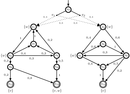
Figure 3: Markov Decision Process

Figure 3 shows a $\operatorname{MDP}$. Absorbing states (i.e., states $s$ with $\tau(s)=\{1_{s}\}$) are represented by double lines. This $\operatorname{MDP}$ features a single nondeterministic decision, to be made in state $s_{0}$, namely $\pi_{1}$ and $\pi_{2}$.

Definition 2.4.

Let $\operatorname{{\cal D}}=(S,s_{0},\tau,L)$ be a $\operatorname{MDP}$ and ${\cal A}\subseteq S$. We define the sets of paths and finite paths reaching ${\cal A}$ as

$$\operatorname{Reach}(\operatorname{{\cal D}},s,{\cal A})\triangleq\{\omega\in\operatorname{Paths}(\operatorname{{\cal D}},s)\mid\exists_{i\geq 0}.\omega_{i}\in{\cal A}\}\mbox{ and}$$

$$\operatorname{Reach}^{\star}(\operatorname{{\cal D}},s,{\cal A})\triangleq\{\sigma\in\operatorname{Paths}^{\star}(\operatorname{{\cal D}},s)\mid\operatorname{last}(\sigma)\in{\cal A}\land\forall_{i\leq|\sigma|-1}.\sigma_{i}\not\in{\cal A}\}$$

respectively. Note that $\operatorname{Reach}^{\star}(\operatorname{{\cal D}},s,{\cal A})$ consists of those finite paths $\sigma$ reaching ${\cal A}$ exactly once, at the end of the execution. It is easy to check that these sets are prefix free, i.e. contain finite paths such that none of them is a prefix of another one.

2.2 Schedulers

Schedulers (also called strategies, adversaries, or policies) resolve the nondeterministic choices in a $\operatorname{MDP}$ [PZ93, Var85, BdA95].

Definition 2.5.

Let $\operatorname{{\cal D}}=(S,s_{0},\tau,L)$ be a $\operatorname{MDP}$. A scheduler $\eta$ on $\operatorname{{\cal D}}$ is a function from $\operatorname{Paths}^{\star}(\operatorname{{\cal D}})$ to $\operatorname{Distr}(\wp(\operatorname{Distr}(S)))$ such that for all $\sigma\in\operatorname{Paths}^{\star}(\operatorname{{\cal D}})$ we have $\eta(\sigma)\in\operatorname{Distr}(\tau(\operatorname{last}(\sigma)))$. We denote the set of all schedulers on $\operatorname{{\cal D}}$ by $\operatorname{Sch}(\operatorname{{\cal D}})$.

Note that our schedulers are randomized, i.e., in a finite path $\sigma$ a scheduler chooses an element of $\tau(\operatorname{last}(\sigma))$ probabilistically. Under a scheduler $\eta$, the probability that the next state reached after the path $\sigma$ is $t$, equals $\sum_{\pi\in\tau(\operatorname{last}(\sigma))}\eta(\sigma)(\pi)\cdot\pi(t)$. In this way, a scheduler induces a probability measure on ${\cal B}_{s}$ as usual.

Definition 2.6.

Let $\operatorname{{\cal D}}$ be a $\operatorname{MDP}$, $s\in S$, and $\eta$ an $s$-scheduler on $\operatorname{{\cal D}}$. We define the probability measure $\mu_{s,\eta}$ as the unique measure on ${\cal B}_{s}$ such that for all $s_{0}s_{1}\ldots s_{n}\in\operatorname{Paths}^{\star}(s)$

$${\mathbf{Pr}}_{s,\eta}({\langle{s_{0}s_{1}\ldots s_{n}}\rangle})=\prod_{i=0}^{n-1}\sum_{\pi\in\tau(s_{i})}\eta(s_{0}s_{1}\ldots s_{i})(\pi)\cdot\pi(s_{i+1}).$$

We now recall the notions of deterministic and memoryless schedulers.

Definition 2.7.

Let $\operatorname{{\cal D}}$ be a $\operatorname{MDP}$, $s\in S$, and $\eta$ an scheduler of $\operatorname{{\cal D}}$. We say that $\eta$ is deterministic if $\eta(\sigma)(\pi_{i})$ is either $0$ or $1$ for all $\pi_{i}\in\tau(\operatorname{last}(\sigma))$ and all $\sigma\in\operatorname{Paths}^{\star}(\operatorname{{\cal D}})$. We say that a scheduler is memoryless if for all finite paths $\sigma_{1},\sigma_{2}$ of $\operatorname{{\cal D}}$ with $\operatorname{last}(\sigma_{1})=\operatorname{last}(\sigma_{2})$ we have $\eta(\sigma_{1})=\eta(\sigma_{2})$

Definition 2.8.

Let $\operatorname{{\cal D}}$ be a $\operatorname{MDP}$, $s\in S$, and $\Delta\in{\cal B}_{s}$. Then the maximal and minimal probabilities of $\Delta$, ${\mathbf{Pr}}^{+}_{s}({\Delta}),{\mathbf{Pr}}^{-}_{s}({\Delta})$, are defined by

$${\mathbf{Pr}}^{+}_{s}({\Delta})\triangleq\sup_{\eta\in\operatorname{Sch}_{s}(\operatorname{{\cal D}})}{\mathbf{Pr}}_{s,\eta}({\Delta})\hskip 14.22636pt\text{and}\hskip 14.22636pt{\mathbf{Pr}}^{-}_{s}({\Delta})\triangleq\inf_{\eta\in\operatorname{Sch}_{s}(\operatorname{{\cal D}})}{\mathbf{Pr}}_{s,\eta}({\Delta}).$$

A scheduler that attains ${\mathbf{Pr}}^{+}_{s}({\Delta})$ or ${\mathbf{Pr}}^{-}_{s}({\Delta})$ is called a maximizing or minimizing scheduler respectively.

A Markov chain ($\operatorname{MC}$) is a $\operatorname{MDP}$ associating exactly one probability distribution to each state. In this way nondeterministic choices are not longer allowed.

Definition 2.9 (Markov chain).

Let $\operatorname{{\cal D}}=(S,s_{0},\tau,L)$ be a $\operatorname{MDP}$. If $|\tau(s)|=1$ for all $s\in S$, then we say that $\operatorname{{\cal D}}$ is a Markov chain ($\operatorname{MC}$).

2.3 Linear Temporal Logic

Linear temporal logic (LTL) [MP91] is a modal temporal logic with modalities referring to time. In LTL is possible to encode formulas about the future of paths: a condition will eventually be true, a condition will be true until another fact becomes true, etc.

Definition 2.10.

LTL is built up from the set of propositional variables ${\cal V}$, the logical connectives $\lnot$, $\land$, and a temporal modal operator by the following grammar:

$$\phi::={\cal V}\mid\lnot\phi\mid\phi\land\phi\mid{\phi}{\cal U}{\phi}.$$

Using these operators we define $\lor,\rightarrow,\lozenge{},$ and $\square{}$ in the standard way.

Definition 2.11.

Let $\operatorname{{\cal D}}=(S,s_{0},\tau,L)$ be a $\operatorname{MDP}$. We define satisfiability for paths $\omega$ in $\operatorname{{\cal D}}$ and LTL formulas $\phi,\psi$ inductively by

$$\begin{array}[]{lcl}\smash{{\omega}\models_{{}_{{}_{{\!\!\operatorname{{\cal D}}}}}}{v}}&\Leftrightarrow&v\in L(\omega_{0})\\ \smash{{\omega}\models_{{}_{{}_{{\!\!\operatorname{{\cal D}}}}}}{\lnot\phi}}&\Leftrightarrow&\mbox{not}(\smash{{\omega}\models_{{}_{{}_{{\!\!\operatorname{{\cal D}}}}}}{\phi}})\\ \smash{{\omega}\models_{{}_{{}_{{\!\!\operatorname{{\cal D}}}}}}{\phi\land\psi}}&\Leftrightarrow&\smash{{\omega}\models_{{}_{{}_{{\!\!\operatorname{{\cal D}}}}}}{\phi}}\mbox{ and }\smash{{\omega}\models_{{}_{{}_{{\!\!\operatorname{{\cal D}}}}}}{\psi}}\\ \smash{{\omega}\models_{{}_{{}_{{\!\!\operatorname{{\cal D}}}}}}{{\phi}{\cal U}{\psi}}}&\Leftrightarrow&\exists_{i\geq 0}.\smash{{\omega_{\downarrow i}}\models_{{}_{{}_{{\!\!\operatorname{{\cal D}}}}}}{\psi}}\mbox{ and }\forall_{0\leq j<i}.\smash{{\omega_{\downarrow j}}\models_{{}_{{}_{{\!\!\operatorname{{\cal D}}}}}}{\phi}}\end{array}$$

where $\omega_{\downarrow i}$ is the $i$-th suffix of $\omega$. When confusion is unlikely, we omit the subscript $\operatorname{{\cal D}}$ on the satisfiability relation.

Definition 2.12.

Let $\operatorname{{\cal D}}$ be a $\operatorname{MDP}$. We define the language $\text{Sat}_{{}_{\operatorname{{\cal D}}}}(\phi)$ associated to an LTL formula $\phi$ as the set of paths satisfying $\phi$, i.e. $\text{Sat}_{{}_{\operatorname{{\cal D}}}}(\phi)\triangleq\{\omega\in\operatorname{Paths}(\operatorname{{\cal D}})\mid\omega\models\phi\}.$ Here we also generally omit the subscript $\operatorname{{\cal D}}$.

We now define satisfiability of an LTL formula $\phi$ on a $\operatorname{MDP}$ $\operatorname{{\cal D}}$. We say that $\operatorname{{\cal D}}$ satisfies $\phi$ with probability at most $p$ ($\smash{{\operatorname{{\cal D}}}\models_{{}_{{}_{{\!\!\leq p}}}}{\phi}}$) if the probability of getting an execution satisfying $\phi$ is at most $p$.

Definition 2.13.

Let $\operatorname{{\cal D}}$ be a $\operatorname{MDP}$, $\phi$ an LTL formula and $p\in[0,1]$. We define $\smash{{}\models_{{}_{{}_{{\!\!\leq p}}}}{}}$ and $\smash{{}\models_{{}_{{}_{{\!\!\geq p}}}}{}}$by

$$\smash{{\operatorname{{\cal D}}}\models_{{}_{{}_{{\!\!\leq p}}}}{\phi}}\Leftrightarrow{\mathbf{Pr}}^{+}_{{}_{\operatorname{{\cal D}}}}({\operatorname{Sat}(\phi)})\leq p,$$

$$\smash{{\operatorname{{\cal D}}}\models_{{}_{{}_{{\!\!\geq p}}}}{\phi}}\Leftrightarrow{\mathbf{Pr}}^{-}_{{}_{\operatorname{{\cal D}}}}({\operatorname{Sat}(\phi)})\geq p.$$

We define $\smash{{\operatorname{{\cal D}}}\models_{{}_{{}_{{\!\!<p}}}}{\phi}}$ and $\smash{{\operatorname{{\cal D}}}\models_{{}_{{}_{{\!\!>p}}}}{\phi}}$ in a similar way.

In case the $\operatorname{MDP}$ is fully probabilistic, i.e., a $\operatorname{MC}$, the satisfiability problem is reduced to $\smash{{\operatorname{{\cal D}}}\models_{{}_{{}_{{\!\!\bowtie p}}}}{\phi}}\Leftrightarrow{\mathbf{Pr}}_{{}_{\operatorname{{\cal D}}}}({\operatorname{Sat}(\phi)})\bowtie p$, where $\bowtie\in\{<,\leq,>,\geq\}$.

3 Counterexamples

In this section, we define what counterexamples are and how the problem of finding counterexamples for a general LTL property over Markov Decision Processes reduces to finding counterexamples to reachability problems over Markov chains.

Definition 3.1 (Counterexamples).

Let $\operatorname{{\cal D}}$ be a $\operatorname{MDP}$ and $\phi$ an LTL formula. A counterexample to $\smash{{\operatorname{{\cal D}}}\models_{{}_{{}_{{\!\!\leq p}}}}{\phi}}$ is a measurable set ${\cal C}\subseteq\operatorname{Sat}(\phi)$ such that ${\mathbf{Pr}}^{+}_{\operatorname{{\cal D}}}({{\cal C}})>p$. Counterexamples to $\smash{{\operatorname{{\cal D}}}\models_{{}_{{}_{{\!\!<p}}}}{\phi}}$ are defined similarly.

Counterexamples to $\smash{{\operatorname{{\cal D}}}\models_{{}_{{}_{{\!\!>p}}}}{\phi}}$ and $\smash{{\operatorname{{\cal D}}}\models_{{}_{{}_{{\!\!\geq p}}}}{\phi}}$ cannot be defined straightforwardly as it is always possible to find a set ${\cal C}\subseteq\operatorname{Sat}(\phi)$ such that ${\mathbf{Pr}}^{-}_{\operatorname{{\cal D}}}({{\cal C}})\leq p$ or ${\mathbf{Pr}}^{-}_{\operatorname{{\cal D}}}({{\cal C}})<p$, note that the empty set trivially satisfies it. Therefore, the best way to find counterexamples to lower bounded probabilities is to find counterexamples to the dual properties $\smash{{\operatorname{{\cal D}}}\models_{{}_{{}_{{\!\!<1-p}}}}{\!\!\!\neg\phi}}$ and $\smash{{\operatorname{{\cal D}}}\models_{{}_{{}_{{\!\!\leq 1-p}}}}{\!\!\!\neg\phi}}$. That is, while for upper bounded probabilities, a counterexample is a set of paths satisfying the property beyond the bound, for lower bounded probabilities the counterexample is a set of paths that does not satisfy the property with sufficient probability.

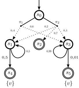
Figure 4:

Example 3. Consider the $\operatorname{MDP}$ $\operatorname{{\cal D}}$ of Figure 4 and the LTL formula $\lozenge{v}$. it is easy to check that $\smash{{\operatorname{{\cal D}}}\not\models_{{}_{{}_{\!\!{<1}}}}{\lozenge{v}}}$. The set ${\cal C}=\operatorname{Sat}(\lozenge{v})=\{\gamma\!\in\!\operatorname{Paths}(s_{0})|\exists_{i\geq 0}.\gamma\!=\!s_{0}(s_{1})^{i}(s_{4})^{\omega}\}\cup\{\gamma\!\in\!\operatorname{Paths}(s_{0})|\exists_{i\geq 0}.\gamma\!=\!s_{0}(s_{3})^{i}(s_{5})^{\omega}\}$ is a counterexample. Note that ${\mathbf{Pr}}^{+}_{s_{0},\eta}({{\cal C}})\!=\!1$ where $\eta$ is any deterministic scheduler of $\operatorname{{\cal M}}$ satisfying $\eta(s_{0})=\pi_{1}$.

LTL formulas are actually checked by reducing the model checking problem to a reachability problem [dAKM97]. For checking upper bounded probabilities, the LTL formula is translated into an equivalent deterministic Rabin automaton and composed with the $\operatorname{MDP}$ under verification. On the obtained $\operatorname{MDP}$, the set of states forming accepting end components (maximal components that traps accepting conditions with probability 1) are identified. The maximum probability of the LTL property on the original $\operatorname{MDP}$ is the same as the maximum probability of reaching a state of an accepting end component in the final $\operatorname{MDP}$. Hence, from now on we will focus on counterexamples to properties of the form $\smash{{\operatorname{{\cal D}}}\models_{{}_{{}_{{\!\!\leq p}}}}{\lozenge{\psi}}}$ or $\smash{{\operatorname{{\cal D}}}\models_{{}_{{}_{{\!\!<p}}}}{\lozenge{\psi}}}$, where $\psi$ is a propositional formula, i.e., a formula without temporal operators.

In the following, it will be useful to identify the set of states in which a propositional property is valid.

Definition 3.2.

Let $\operatorname{{\cal D}}$ be a $\operatorname{MDP}$. We define the state language $\text{Sat}_{\operatorname{{\cal D}}}(\psi)$ associated to a propositional formula $\psi$ as the set of states satisfying $\psi$, i.e., $\text{Sat}_{\operatorname{{\cal D}}}(\psi)\triangleq\{s\in S\mid s\models\psi\}$, where $\models$ has the obvious satisfaction meaning for states. As usual, we generally omit the subscript $\operatorname{{\cal D}}$.

To find a counterexample to a property in a $\operatorname{MDP}$ with respect to a upper bound, it suffices to find a counterexample for the maximizing scheduler. A scheduler defines a Markov chain, and hence finding a counterexample on a $\operatorname{MDP}$ amounts to finding a counterexample in the Markov chain induced by the maximizing scheduler. The maximizing scheduler turns out to be deterministic and memoryless [BdA95]; consequently the induced Markov chain can be easily extracted from the $\operatorname{MDP}$ as follows.

Definition 3.3.

Let $\operatorname{{\cal D}}=(S,s_{0},\tau,L)$ be a $\operatorname{MDP}$ and $\eta$ a deterministic memoryless scheduler. Then we define the $\operatorname{MC}$ $\eta$-associated to $\operatorname{{\cal D}}$ as $\operatorname{{\cal D}}_{\eta}=(S,s_{0},{\cal P}_{\eta},L)$ where ${\cal P}_{\eta}(s,t)=(\eta(s))(t)$ for all $s,t\in S$.

Now we state that finding counterexamples for upper bounded probabilistic reachability LTL properties on $\operatorname{MDPs}$ can be reduced to finding counterexamples for upper bounded probabilistic reachability LTL properties on $\operatorname{MCs}$.

Theorem 3.4.

Let $\operatorname{{\cal D}}$ be a $\operatorname{MDP}$, $\psi$ a propositional formula and $p\in[0,1]$. Then, there is a maximizing (deterministic memoryless) scheduler $\eta$ such that $\smash{{\operatorname{{\cal D}}}\models_{{}_{{}_{{\!\!\leq p}}}}{\lozenge{\psi}}}\Leftrightarrow\smash{{\operatorname{{\cal D}}_{\eta}}\models_{{}_{{}_{{\!\!\leq p}}}}{\lozenge{\psi}}}$. Moreover, ${\cal C}$ is a counterexample to $\smash{{\operatorname{{\cal D}}_{\eta}}\models_{{}_{{}_{{\!\!\leq p}}}}{\lozenge{\psi}}}$ if and only if ${\cal C}$ is also a counterexample to $\smash{{\operatorname{{\cal D}}}\models_{{}_{{}_{{\!\!\leq p}}}}{\lozenge{\psi}}}$.

4 Representative Counterexamples, Partitions and Witnesses

The notion of counterexample from Definition 3.1 is very broad: just an arbitrary (measurable) set of paths with high enough probability. To be useful as a debugging tool (and in fact to be able to present the counterexample to a user), we need counterexamples with specific properties. We will partition counterexamples (or rather, representative counterexamples) in witnesses and list five properties that witnesses should satisfy.

The first point to stress is that for reachability properties it is sufficient to consider counterexamples that consist of finite paths.

Definition 4.1 (Representative counterexamples).

Let $\operatorname{{\cal D}}$ be a $\operatorname{MDP}$, $\psi$ a propositional formula and $p\in[0,1]$. A representative counterexample to $\smash{{\operatorname{{\cal D}}}\models_{{}_{{}_{{\!\!\leq p}}}}{\lozenge{\psi}}}$ is a set ${\cal C}\subseteq\operatorname{Reach}^{\star}(\operatorname{{\cal D}},\operatorname{Sat}(\psi))$ such that ${\mathbf{Pr}}^{+}_{\operatorname{{\cal D}}}({\langle{{\cal C}}\rangle})>p$. We denote the set of all representative counterexamples to $\smash{{\operatorname{{\cal M}}}\models_{{}_{{}_{{\!\!\leq p}}}}{\lozenge{\psi}}}$ by ${\cal R}({\operatorname{{\cal M}},p,\psi})$.

Theorem 4.2.

Let $\operatorname{{\cal D}}$ be a $\operatorname{MDP}$, $\psi$ a propositional formula and $p\in[0,1]$. If ${\cal C}$ is a representative counterexample to $\smash{{\operatorname{{\cal D}}}\models_{{}_{{}_{{\!\!\leq p}}}}{\lozenge{\psi}}}$, then $\langle{{\cal C}}\rangle$ is a counterexample to $\smash{{\operatorname{{\cal D}}}\models_{{}_{{}_{{\!\!\leq p}}}}{\lozenge{\psi}}}$. Furthermore, there exists a counterexample to $\smash{{\operatorname{{\cal D}}}\models_{{}_{{}_{{\!\!\leq p}}}}{\lozenge{\psi}}}$ if and only if there exists a representative counterexample to $\smash{{\operatorname{{\cal D}}}\models_{{}_{{}_{{\!\!\leq p}}}}{\psi}}$.

Following [HK07a], we present the notions of minimum counterexample, strongest evidence and most indicative counterexamples.

Definition 4.3 (Minimum counterexample).

Let $\operatorname{{\cal M}}$ be a $\operatorname{MC}$, $\psi$ a propositional formula and $p\in[0,1]$. We say that ${\cal C}\in{\cal R}({\operatorname{{\cal M}},p,\psi})$ is a minimum counterexample if $|{\cal C}|\leq|{\cal C}^{\prime}|$, for all ${\cal C}^{\prime}\in{\cal R}({\operatorname{{\cal M}},p,\psi})$.

Definition 4.4 (Strongest evidence).

Let $\operatorname{{\cal M}}$ be a $\operatorname{MC}$, $\psi$ a propositional formula and $p\in[0,1]$. A strongest evidence to $\smash{\smash{{\operatorname{{\cal M}}}\not\models_{{}_{{}_{\!\!{\leq p}}}}{\lozenge{\psi}}}}$ is a finite path $\sigma\in\operatorname{Reach}^{\star}(\operatorname{{\cal M}},\operatorname{Sat}(\psi))$ such that ${\mathbf{Pr}}_{\operatorname{{\cal M}}}({\langle{\sigma}\rangle})\geq{\mathbf{Pr}}_{\operatorname{{\cal M}}}({\langle{\rho}\rangle})$, for all $\rho\in\operatorname{Reach}^{\star}(\operatorname{{\cal M}},\operatorname{Sat}(\psi))$.

Definition 4.5 (Most indicative counterexample).

Let $\operatorname{{\cal M}}$ be a $\operatorname{MC}$, $\psi$ a propositional formula and $p\in[0,1]$. We call ${\cal C}\in{\cal R}({\operatorname{{\cal M}},p,\psi})$ a most indicative counterexample if it is minimum and ${\mathbf{Pr}}({\langle{{\cal C}}\rangle})\geq{\mathbf{Pr}}({\langle{{\cal C}^{\prime}}\rangle})$, for all minimum counterexamples ${\cal C}^{\prime}\in{\cal R}({\operatorname{{\cal M}},p,\psi})$.

Unfortunately, very often most indicative counterexamples are very large (even infinite), many of its elements have insignificant measure and elements can be extremely similar to each other (consequently providing the same diagnostic information). Even worse, sometimes the finite paths with highest probability do not exhibit the way in which the system accumulates higher probability to reach the undesired property (and consequently where an error occurs with higher probability). For these reasons, we are of the opinion that representative counterexamples are still too general in order to be useful as feedback information. We approach this problem by splitting out the representative counterexample into sets of finite paths following a “similarity” criteria (introduced in Section 5). These sets are called witnesses of the counterexample.

Recall that a set $Y$ of nonempty sets is a partition of $X$ if the elements of $Y$ cover $X$ and the elements of $Y$ are pairwise disjoint. We define counterexample partitions in the following way.

Definition 4.6 (Counterexample partitions and witnesses).

Let $\operatorname{{\cal D}}$ be a $\operatorname{MDP}$, $\psi$ a propositional formula, $p\in[0,1]$, and ${\cal C}$ a representative counterexample to $\smash{{\operatorname{{\cal D}}}\models_{{}_{{}_{{\!\!\leq p}}}}{\lozenge{\psi}}}$. A counterexample partition $W_{\cal C}$ is a partition of ${\cal C}$. We call the elements of $W_{\cal C}$ witnesses.

Since not every partition generates useful witnesses (from the debugging perspective), we now state properties that witnesses must satisfy in order to be valuable as diagnostic information. In Section 7 we show how to partition the detailed counterexample in order to obtain useful witnesses.

• Elements of a witness should provide similar debugging information.

• Witnesses with higher probability should show evolution of the system with higher probability of containing errors.

• Different witnesses should provide different debugging information.

• The probability of a witnesses should be close to the probability bound $p$.

• The number of witnesses of a counterexamples partition should be finite.

5 Rails and Torrents

As argued before we consider that representative counterexamples are excessively general to be useful as feedback information. Therefore, we group finite paths of a representative counterexample in witnesses if they are “similar enough”. We will consider finite paths that behave the same outside $\operatorname{SCCs}$ of the system as providing similar feedback information.

In order to formalize this idea, we first reduce the original Markov chain to an acyclic one that preserves reachability probabilities. We do so by removing all $\operatorname{SCCs}$ $\operatorname{K}$ of $\operatorname{{\cal M}}$ keeping just input states of $\operatorname{K}$. In this way, we get a new acyclic $\operatorname{MC}$ denoted by $\operatorname{Ac}(\operatorname{{\cal M}})$. The probability matrix of the Markov chain relates input states of each $\operatorname{SCC}$ with its output states with the reachability probability between these states in $\operatorname{{\cal M}}$. Secondly, we establish a map between finite paths $\sigma$ in $\operatorname{Ac}(\operatorname{{\cal M}})$ (rails) and sets of finite paths $W_{\sigma}$ in $\operatorname{{\cal M}}$ (torrents). Each torrent contains finite paths that are similar, i.e., behave the same outside $\operatorname{SCCs}$. Additionally we show that the probability of $\sigma$ is equal to the probability of $W_{\sigma}$.

Reduction to Acyclic Markov Chains

Consider a $\operatorname{MC}$ $\operatorname{{\cal M}}=(S,s_{0},{\cal P},L)$. Recall that a subset $\operatorname{K}\subseteq S$ is called strongly connected if for every $s,t\in\operatorname{K}$ there is a finite path from $s$ to $t$. Additionally $\operatorname{K}$ is called a strongly connected component ($\operatorname{SCC}$) if it is a maximally (with respect to $\subseteq$) strongly connected subset of $S$.

Note that every state is a member of exactly one $\operatorname{SCC}$ of $\operatorname{{\cal M}}$ (even those states that are not involved in cycles, since the trivial finite path $s$ connects $s$ to itself). From now on we let $\operatorname{SCC}^{\star}$ be the set of non trivial strongly connected components of a $\operatorname{MC}$, i.e., those composed of more than one state.

A Markov chain is called acyclic if it does not have non trivial $\operatorname{SCCs}$. Note that an acyclic Markov chain still has absorbing states.

Definition 5.1.

Let $\operatorname{{\cal M}}=(S,s_{0},{\cal P},L)$ be a $\operatorname{MC}$. Then, for each $\operatorname{SCC}^{\star}$ $\operatorname{K}$ of $\operatorname{{\cal M}}$, we define the sets $\operatorname{Inp}_{\operatorname{K}}\subseteq S$ of all states in $\operatorname{K}$ that have an incoming transition from a state outside of $\operatorname{K}$ and $\operatorname{Out}_{\operatorname{K}}\subseteq S$ of all states outside of $\operatorname{K}$ that have an incoming transition from a state of $\operatorname{K}$ in the following way

$$\operatorname{Inp}_{\operatorname{K}}\triangleq\{u\in\operatorname{K}\mid\exists\,s\in S\setminus\operatorname{K}.{\cal P}(s,u)>0\},$$

$$\operatorname{Out}_{\operatorname{K}}\triangleq\{s\in S\setminus\operatorname{K}\mid\exists\,u\in\operatorname{K}.{\cal P}(u,s)>0\}.$$

We also define for each $\operatorname{SCC}^{\star}$ $\operatorname{K}$ a $\operatorname{MC}$ related to $\operatorname{K}$ as $\operatorname{{\cal M}}_{\operatorname{K}}\triangleq(\operatorname{K}\cup\operatorname{Out}_{\operatorname{K}},s_{\operatorname{K}},{\cal P}_{\operatorname{K}},L_{\operatorname{K}})$ where $s_{\operatorname{K}}$ is any state in $\operatorname{Inp}_{\operatorname{K}}$, $L_{\operatorname{K}}(s)\triangleq L(s)$, and ${\cal P}_{\operatorname{K}}(s,t)$ is equal to ${\cal P}(s,t)$ if $s\in\operatorname{K}$ and equal to $1_{s}$ otherwise. Additionally, for every state $s$ involved in non trivial $\operatorname{SCCs}$ we define $\operatorname{SCC}^{+}_{s}$ as $\operatorname{{\cal M}}_{\operatorname{K}}$, where $\operatorname{K}$ is the $\operatorname{SCC}^{\star}$ of $\operatorname{{\cal M}}$ such that $s\in\operatorname{K}$.

Now we are able to define an acyclic $\operatorname{MC}$ $\operatorname{Ac}(\operatorname{{\cal M}})$ related to $\operatorname{{\cal M}}$.

Definition 5.2.

Let $\operatorname{{\cal M}}=(S,s_{0},{\cal P},L)$ be a $\operatorname{MC}$. We define $\operatorname{Ac}(\operatorname{{\cal M}}){}\triangleq(S^{\prime},s_{0},{\cal P}^{\prime}{},L^{\prime})$ where

• $S^{\prime}\triangleq\stackrel{{\scriptstyle S_{\text{com}}}}{{\overbrace{S\setminus\bigcup_{\operatorname{K}\in\operatorname{SCC}^{\star}}\operatorname{K}}}}\bigcup\stackrel{{\scriptstyle S_{\text{inp}}}}{{\overbrace{\bigcup_{\operatorname{K}\in\operatorname{SCC}^{\star}}\operatorname{Inp}_{\operatorname{K}}}}}$

• $L^{\prime}\triangleq L_{|_{S^{\prime}}}$,

• ${\cal P}^{\prime}(s,t)\triangleq\left\{\begin{array}[]{ll}{\cal P}(s,t)&\mbox{if }s\in S_{com},\\ {\mathbf{Pr}}_{{}_{\operatorname{{\cal M}},s}}({\operatorname{Reach}(\operatorname{SCC}^{+}_{s},s,\{t\})})&\mbox{if }s\in S_{inp}\land t\in\operatorname{Out}_{\operatorname{SCC}^{+}_{s}},\\ 1_{s}&\mbox{if }s\in S_{inp}\land\operatorname{Out}_{\operatorname{SCC}^{+}_{s}}=\emptyset,\\ 0&\mbox{otherwise.}\end{array}\right.$

Note that $\operatorname{Ac}(\operatorname{{\cal M}})$ is indeed acyclic.

Example 2.

Consider the $\operatorname{MC}$ $\operatorname{{\cal M}}$ of Figure 5(a). The strongly connected components of $\operatorname{{\cal M}}$ are $\operatorname{K}_{1}\triangleq\{s_{1},s_{3},s_{4},s_{7}\}$, $\operatorname{K}_{2}\triangleq\{s_{5},s_{6},s_{8}\}$ and the singletons $\{s_{0}\}$, $\{s_{2}\}$, $\{s_{9}\}$, $\{s_{10}\}$, $\{s_{11}\}$, $\{s_{12}\}$, $\{s_{13}\}$, and $\{s_{14}\}$. The input states of $\operatorname{K}_{1}$ are $\operatorname{Inp}_{\operatorname{K}_{1}}=\{s_{1}\}$ and its output states are $\operatorname{Out}_{\operatorname{K}_{1}}=\{s_{9},s_{10}\}$. For $\operatorname{K}_{2}$, $\operatorname{Inp}_{\operatorname{K}_{2}}=\{s_{5},s_{6}\}$ and $\operatorname{Out}_{\operatorname{K}_{2}}=\{s_{11},s_{14}\}$. The reduced acyclic $\operatorname{MC}$ of $\operatorname{{\cal M}}$ is shown in Figure 5(b).

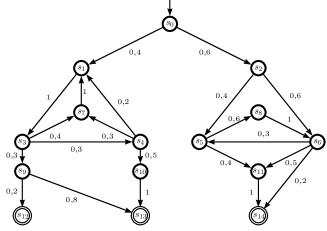
(a) Original $\operatorname{MC}$

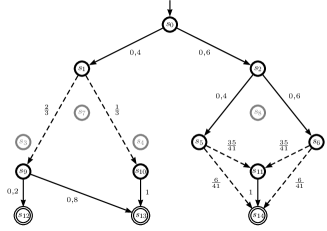
(b) Derived Acyclic $\operatorname{MC}$

Figure 5:

Rails and Torrents

We now relate (finite) paths in $\operatorname{Ac}(\operatorname{{\cal M}})$ (rails) to sets of (finite) paths in $\operatorname{{\cal M}}$ (torrents).

Definition 5.3 (Rails).

Let $\operatorname{{\cal M}}$ be a $\operatorname{MC}$. A finite path $\sigma\in\operatorname{Paths}^{\star}(\operatorname{Ac}(\operatorname{{\cal M}}))$ will be called a rail of $\operatorname{{\cal M}}$.

Consider a rail $\sigma$, i.e., a finite path of $\operatorname{Ac}(\operatorname{{\cal M}})$. We will use $\sigma$ to represent those paths $\omega$ of $\operatorname{{\cal M}}$ that behave “similar to” $\sigma$ outside $\operatorname{SCCs}$ of $\operatorname{{\cal M}}$. Naively, this means that $\sigma$ is a subsequence of $\omega$. There are two technical subtleties to deal with: every input state in $\sigma$ must be the first state in its $\operatorname{SCC}$ in $\omega$ (freshness) and every $\operatorname{SCC}$ visited by $\omega$ must be also visited by $\sigma$ (inertia) (see Definition 5.5). We need these extra conditions to make sure that no path $\omega$ behaves “similar to” two distinct rails (see Lemma 5.7).

Recall that given a finite sequence $\sigma$ and a (possible infinite) sequence $\omega$, we say that $\sigma$ is a subsequence of $\omega$, denoted by $\sigma\sqsubseteq\omega$, if and only if there exists a strictly increasing function $f:\{0,1,\ldots,|\sigma|-1\}\rightarrow\{0,1,\ldots,|\omega|-1\}$ such that $\forall_{0\leq i<|\sigma|}.\sigma_{i}=\omega_{f(i)}$. If $\omega$ is an infinite sequence, we interpret the codomain of $f$ as $\mathbb{N}$. In case $f$ is such a function we write $\sigma\sqsubseteq_{f}\omega$. Note that finite paths and paths are sequences.

Definition 5.4.

Let $\operatorname{{\cal M}}=(S,s_{0},{\cal P},L)$ be a $\operatorname{MC}$. On $S$ we consider the equivalence relation $\sim_{\!\!\!\!\!\!{}_{\operatorname{{\cal M}}}}$ satisfying $s\sim_{\!\!\!\!\!\!{}_{\operatorname{{\cal M}}}}t$ if and only if $s$ and $t$ are in the same strongly connected component. Again, we usually omit the subscript $\operatorname{{\cal M}}$ from the notation.

The following definition refines the notion of subsequence, taking care of the two technical subtleties noted above.

Definition 5.5.

Let $\operatorname{{\cal M}}=(S,s_{0},{\cal P},L)$ be a $\operatorname{MC}$, $\omega$ a (finite) path of $\operatorname{{\cal M}}$, and $\sigma\in\operatorname{Paths}^{\star}(\operatorname{Ac}(\operatorname{{\cal M}}))$ a finite path of $\operatorname{Ac}(\operatorname{{\cal M}})$. Then we write $\sigma\preceq\omega$ if there exists $f:\{0,1,\ldots,|\sigma|-1\}\rightarrow\mathbb{N}$ such that $\sigma\sqsubseteq_{f}\omega$ and for all $0\leq i<|\sigma|$ we have

$$\forall_{0\leq j<f(i)}:\omega_{f(i)}\not\sim\omega_{j} \mbox{; for all }i=0,1,\ldots|\sigma|-1, [\mbox{\emph{Freshness property}}]$$

$$\forall_{f(i)<j<f(i+1)}:\omega_{f(i)}\sim\omega_{j} \mbox{; for all }i=0,1,\ldots|\sigma|-2. [\mbox{\emph{Inertia property}}]$$

In case $f$ is such a function we write $\sigma\preceq_{f}\omega$.

Example 3.

Let $\operatorname{{\cal M}}=(S,s_{0},{\cal P},L)$ be the $\operatorname{MC}$ of Figure 5(a) and take $\sigma=s_{0}s_{2}s_{6}s_{14}$. Then for all $i\in\mathbb{N}$ we have $\sigma\preceq_{f_{i}}\omega_{i}$ where $\omega_{i}=s_{0}s_{2}s_{6}(s_{5}s_{8}s_{6})^{i}s_{14}$ and $f_{i}(0)\triangleq 0$, $f_{i}(1)\triangleq 1$, $f_{i}(2)\triangleq 2$, and $f_{i}(3)\triangleq 3+3i$. Additionally, $\sigma\not\preceq s_{0}s_{2}s_{5}s_{8}s_{6}s_{14}$ since for all $f$ satisfying $\sigma\sqsubseteq_{f}s_{0}s_{2}s_{5}s_{8}s_{6}s_{14}$ we must have $f(2)=5$; this implies that $f$ does not satisfy the freshness property. Finally, note that $\sigma\not\preceq s_{0}s_{2}s_{6}s_{11}s_{14}$ since for all $f$ satisfying $\sigma\sqsubseteq_{f}s_{0}s_{2}s_{6}s_{11}s_{14}$ we must have $f(2)=2$; this implies that $f$ does not satisfy the inertia property.

We now give the formal definition of torrents.

Definition 5.6 (Torrents).

Let $\operatorname{{\cal M}}=(S,s_{0},{\cal P},L)$ be a $\operatorname{MC}$ and $\sigma$ a sequence of states in $S$. We define the function Torr by

$$\operatorname{Torr}({\operatorname{{\cal M}},\sigma})\triangleq\{\omega\in\operatorname{Paths}(\operatorname{{\cal M}})\mid\sigma\preceq\omega\}.$$

We call $\operatorname{Torr}({\operatorname{{\cal M}},\sigma})$ the torrent associated to $\sigma$.

We now show that torrents are disjoint (Lemma 5.7) and that the probability of a rail is equal to the probability of its associated torrent (Theorem 5.10). For this last result, we first show that torrents can be represented as the disjoint union of cones of finite paths. We call these finite paths generators of the torrent (Definition 5.8).

Lemma 5.7.

Let $\operatorname{{\cal M}}$ be a $\operatorname{MC}$. For every $\sigma,\rho\in\operatorname{Paths}^{\star}(\operatorname{Ac}(\operatorname{{\cal M}}))$ we have

$$\sigma\not=\rho\Rightarrow\operatorname{Torr}({\operatorname{{\cal M}},\sigma})\cap\operatorname{Torr}({\operatorname{{\cal M}},\rho})=\emptyset$$

Definition 5.8 (Torrent Generators).

Let $\operatorname{{\cal M}}$ be a $\operatorname{MC}$. Then we define for every rail $\sigma\in\operatorname{Paths}^{\star}(\operatorname{Ac}(\operatorname{{\cal M}}))$ the set

$$\operatorname{GenTorr}(\operatorname{{\cal M}},\sigma)\triangleq\{\rho\in\operatorname{Paths}^{\star}(\operatorname{{\cal M}})\mid\exists f:\sigma\preceq_{f}\rho\land f(|\sigma|-1)=|\rho|-1\}.$$

In the example from the Introduction (see Figure 2), $s_{0}s_{1}s_{3}$ and $s_{0}s_{2}s_{4}$ are rails. The associated torrents are, respectively, $\{s_{0}s_{1}^{n}s_{3}^{\omega}\;|\;n\in{\mathbb{N}}^{*}\}$ and $\{s_{0}s_{2}^{n}s_{4}^{\omega}\;|\;n\in{\mathbb{N}}^{*}\}$ (note that $s_{3}$ and $s_{4}$ are absorbing states), i.e. the paths going left and the paths going right. The generators of the first torrent are $\{s_{0}s_{1}^{n}s_{3}\;|\;n\in{\mathbb{N}}^{*}\}$ and similarly for the second torrent.

Lemma 5.9.

Let $\operatorname{{\cal M}}$ be a $\operatorname{MC}$ and $\sigma\in\operatorname{Paths}^{\star}(\operatorname{Ac}(\operatorname{{\cal M}}))$ a rail of $\operatorname{{\cal M}}$. Then we have

$$\operatorname{Torr}({\operatorname{{\cal M}},\sigma})=\biguplus_{\rho\in\operatorname{GenTorr}(\operatorname{{\cal M}},\sigma)}\langle{\rho}\rangle.$$

Theorem 5.10.

Let $\operatorname{{\cal M}}$ be a $\operatorname{MC}$. Then for every rail $\sigma\in\operatorname{Paths}^{\star}(\operatorname{Ac}(\operatorname{{\cal M}}))$ we have

$${\mathbf{Pr}}_{{}_{\operatorname{Ac}(\operatorname{{\cal M}})}}({\langle{\sigma}\rangle})={\mathbf{Pr}}_{{}_{\operatorname{{\cal M}}}}({\operatorname{Torr}({\operatorname{{\cal M}},\sigma})}).$$

6 Significant Diagnostic Counterexamples

So far we have formalized the notion of paths behaving similarly (i.e., behaving the same outside $\operatorname{SCCs}$) in a $\operatorname{MC}$ $\operatorname{{\cal M}}$ by removing all $\operatorname{SCC}$ of $\operatorname{{\cal M}}$, obtaining $\operatorname{Ac}(\operatorname{{\cal M}})$. A representative counterexample to $\smash{{\operatorname{Ac}(\operatorname{{\cal M}})}\models_{{}_{{}_{{\!\!\leq p}}}}{\lozenge{\psi}}}$ will give rise to a representative counterexample to $\smash{{\operatorname{{\cal M}}}\models_{{}_{{}_{{\!\!\leq p}}}}{\lozenge{\psi}}}$. For every finite path $\sigma$ in the counterexample to $\smash{{\operatorname{Ac}(\operatorname{{\cal M}})}\models_{{}_{{}_{{\!\!\leq p}}}}{\lozenge{\psi}}}$, the set $\operatorname{GenTorr}(\operatorname{{\cal M}},\sigma)$ will be a witness. The union of these is the representative counterexample to $\smash{{\operatorname{{\cal M}}}\models_{{}_{{}_{{\!\!\leq p}}}}{\lozenge{\psi}}}$.

Before giving a formal definition, there is still one technical issue to resolve: we need to be sure that by removing $\operatorname{SCCs}$ we are not discarding useful information. Because torrents are built from rails, we need to make sure that when we discard $\operatorname{SCCs}$, we do not discard rails that reach $\psi$.

We achieve this by first making states satisfying $\psi$ absorbing. Additionally, we make absorbing states from which it is not possible to reach $\psi$. Note that this does not affect counterexamples.

Definition 6.1.

Let $\operatorname{{\cal M}}=(S,s_{0},{\cal P},L)$ be a $\operatorname{MC}$ and $\psi$ a propositional formula. We define the $\operatorname{MC}$ $\operatorname{{\cal M}}_{\psi}\triangleq(S,s_{0},{\cal P}_{\psi},L)$, with

$${\cal P}_{\psi}(s,t)\triangleq\left\{\begin{array}[]{ll}1&\mbox{if }s\not\in\operatorname{Sat}_{\!{}_{\lozenge}}({\psi})\land s=t,\\ 1&\mbox{if }s\in\operatorname{Sat}(\psi)\land s=t,\\ {\cal P}(s,t)&\mbox{if }s\in\operatorname{Sat}_{\!{}_{\lozenge}}({\psi})-\operatorname{Sat}(\psi),\\ 0&\mbox{otherwise,}\\ \end{array}\right.$$

where $\operatorname{Sat}_{\!{}_{\lozenge}}({\psi})\triangleq\{\allowbreak s\in S\mid\allowbreak\allowbreak{\mathbf{Pr}}_{s}({\operatorname{Reach}(\operatorname{{\cal M}},s,\allowbreak\operatorname{Sat}(\psi))})\allowbreak>0\}$ is the set of states reaching $\psi$ in $\operatorname{{\cal M}}$.

The following theorem shows the relation between paths, finite paths, and probabilities of $\operatorname{{\cal M}}$, $\operatorname{{\cal M}}_{\psi}$, and $\operatorname{Ac}(\operatorname{{\cal M}}_{\psi})$. Most importantly, the probability of a rail $\sigma$ (in $\operatorname{Ac}(\operatorname{{\cal M}}_{\psi})$) is equal to the probability of its associated torrent (in $\operatorname{{\cal M}}$) (item 5 below) and the probability of $\lozenge{\psi}$ is not affected by reducing $\operatorname{{\cal M}}$ to $\operatorname{Ac}(\operatorname{{\cal M}}_{\psi})$ (item 6 below).

Note that a rail $\sigma$ is always a finite path in $\operatorname{Ac}(\operatorname{{\cal M}}_{\psi})$, but that we can talk about its associated torrent $\operatorname{Torr}({\operatorname{{\cal M}}_{\psi},\sigma})$ in $\operatorname{{\cal M}}_{\psi}$ and about its associated torrent $\operatorname{Torr}({\operatorname{{\cal M}},\sigma})$ in $\operatorname{{\cal M}}$. The former exists for technical convenience; it is the latter that we are ultimately interested in. The following theorem also shows that for our purposes, viz. the definition of the generators of the torrent and the probability of the torrent, there is no difference (items 3 and 4 below).

Theorem 6.2.

Let $\operatorname{{\cal M}}=(S,s_{0},{\cal P},L)$ be a $\operatorname{MC}$ and $\psi$ a propositional formula. Then for every $\sigma\in\operatorname{Paths}^{\star}(\operatorname{{\cal M}}_{\psi})$

1. $\operatorname{Reach}^{\star}(\operatorname{{\cal M}}_{\psi},s_{0},\operatorname{Sat}(\psi))=\operatorname{Reach}^{\star}(\operatorname{{\cal M}},s_{0},\operatorname{Sat}(\psi))$,

2. ${\mathbf{Pr}}_{{}_{\operatorname{{\cal M}}_{\psi}}}({\langle{\sigma}\rangle})={\mathbf{Pr}}_{{}_{\operatorname{{\cal M}}}}({\langle{\sigma}\rangle})$,

3. $\operatorname{GenTorr}(\operatorname{{\cal M}}_{\psi},\sigma)=\operatorname{GenTorr}(\operatorname{{\cal M}},\sigma)$,

4. ${\mathbf{Pr}}_{{}_{\operatorname{{\cal M}}_{\psi}}}({\operatorname{Torr}({\operatorname{{\cal M}}_{\psi},\sigma})})={\mathbf{Pr}}_{{}_{\operatorname{{\cal M}}}}({\operatorname{Torr}({\operatorname{{\cal M}},\sigma})})$,

5. ${\mathbf{Pr}}_{\!{}_{\operatorname{Ac}(\operatorname{{\cal M}}_{\psi})}\!}({\langle{\sigma}\rangle})={\mathbf{Pr}}_{{}_{\operatorname{{\cal M}}}}({\operatorname{Torr}({\operatorname{{\cal M}},\sigma})})$,

6. $\smash{{\operatorname{Ac}(\operatorname{{\cal M}}_{\psi})}\models_{{}_{{}_{{\!\!\leq p}}}}{\lozenge{\psi}}}$ if and only if $\smash{{\operatorname{{\cal M}}}\models_{{}_{{}_{{\!\!\leq p}}}}{\lozenge{\psi}}}$, for any $p\in[0,1]$.

Definition 6.3 (Torrent-Counterexamples).

Let $\operatorname{{\cal M}}=(S,s_{0},{\cal P},L)$ be a $\operatorname{MC}$, $\psi$ a propositional formula, and $p\in[0,1]$ such that $\smash{{\operatorname{{\cal M}}}\not\models_{{}_{{}_{\!\!{\leq p}}}}{\lozenge{\psi}}}$. Let ${\cal C}$ be a representative counterexample to $\smash{{\operatorname{Ac}(\operatorname{{\cal M}}_{\psi})}\models_{{}_{{}_{{\!\!\leq p}}}}{\lozenge{\psi}}}$. We define the set

$$\operatorname{TorRepCount}({\cal C})\triangleq\{\operatorname{GenTorr}(\operatorname{{\cal M}},\sigma)\mid\sigma\in{\cal C}\}.$$

We call the set $\operatorname{TorRepCount}({\cal C})$ a torrent-counterexample of ${\cal C}$. Note that this set is a partition of a counterexample to $\smash{{\operatorname{{\cal M}}}\models_{{}_{{}_{{\!\!\leq p}}}}{\lozenge{\psi}}}$. Additionally, we denote by ${\cal R}_{t}({\operatorname{{\cal M}},p,\psi})$ to the set of all torrent-counterexamples to $\smash{{\operatorname{{\cal M}}}\models_{{}_{{}_{{\!\!\leq p}}}}{\lozenge{\psi}}}$, i.e., $\{\operatorname{TorRepCount}({\cal C})\mid{\cal C}\in{\cal R}({\operatorname{{\cal M}},p,\psi})\}$.

Theorem 6.4.

Let $\operatorname{{\cal M}}=(S,s_{0},{\cal P},L)$ be a $\operatorname{MC}$, $\psi$ a propositional formula, and $p\in[0,1]$ such that $\smash{{\operatorname{{\cal M}}}\not\models_{{}_{{}_{\!\!{\leq p}}}}{\lozenge{\psi}}}$. Take ${\cal C}$ a representative counterexample to $\smash{{\operatorname{Ac}(\operatorname{{\cal M}}_{\psi})}\models_{{}_{{}_{{\!\!\leq p}}}}{\lozenge{\psi}}}$. Then the set of finite paths $\biguplus_{W\in\operatorname{TorRepCount}({\cal C})}W$ is a representative counterexample to $\smash{{\operatorname{{\cal M}}}\models_{{}_{{}_{{\!\!\leq p}}}}{\lozenge{\psi}}}$.

Note that for each $\sigma\in{\cal C}$ we get a witness $\operatorname{GenTorr}(\operatorname{{\cal M}},\sigma)$. Also note that the number of rails is finite, so there are also only finitely many witnesses.

Following [HK07a], we extend the notions of minimum counterexamples, strongest evidence and smallest counterexample to torrents.

Definition 6.5 (Minimum torrent-counterexample).

Let $\operatorname{{\cal M}}$ be a $\operatorname{MC}$, $\psi$ a propositional formula and $p\in[0,1]$. We say that ${\cal C}_{t}\in{\cal R}_{t}({\operatorname{{\cal M}},p,\psi})$ is a minimum torrent-counterexample if $|{\cal C}_{t}|\leq|{\cal C}_{t}^{\prime}|$, for all ${\cal C}^{\prime}_{t}\in{\cal R}_{t}({\operatorname{{\cal M}},p,\psi})$.

Definition 6.6 (Strongest torrent-evidence).

Let $\operatorname{{\cal M}}$ be a $\operatorname{MC}$, $\psi$ a propositional formula and $p\in[0,1]$. A strongest torrent-evidence to $\smash{\smash{{\operatorname{{\cal M}}}\not\models_{{}_{{}_{\!\!{\leq p}}}}{\lozenge{\psi}}}}$ is a torrent $W_{\sigma}\in\operatorname{Torr}({\operatorname{{\cal M}},\operatorname{Sat}(\psi)})$ such that ${\mathbf{Pr}}_{\operatorname{{\cal M}}}({W_{\sigma}})\geq{\mathbf{Pr}}_{\operatorname{{\cal M}}}({W_{\rho}})$ for all $W_{\rho}\in\operatorname{Torr}({\operatorname{{\cal M}},\operatorname{Sat}(\psi)})$.

Now we define our notion of significant diagnostic counterexamples. It is the generalization of most indicative counterexample from [HK07a] to our setting.

Definition 6.7 (Most indicative torrent-counterexample).

Let $\operatorname{{\cal M}}$ be a $\operatorname{MC}$, $\psi$ a propositional formula and $p\in[0,1]$. We call ${\cal C}_{t}\in{\cal R}_{t}({\operatorname{{\cal M}},p,\psi})$ a most indicative torrent-counterexample if it is a minimum torrent-counterexample and ${\mathbf{Pr}}({\bigcup_{W\in{\cal C}_{t}}\langle{W}\rangle})\geq{\mathbf{Pr}}({\bigcup_{W\in{\cal C}^{\prime}_{t}}\langle{W}\rangle})$ for all minimum torrent counterexamples ${\cal C}^{\prime}_{t}\in{\cal R}_{t}({\operatorname{{\cal M}},p,\psi})$.

By Theorem 6.4 it is possible to obtain strongest torrent-evidence and most indicative torrent-counterexamples of a $\operatorname{MC}$ $\operatorname{{\cal M}}$ by obtaining strongest evidence and most indicative counterexamples of $\operatorname{Ac}(\operatorname{{\cal M}}_{\psi})$ respectively.

7 Computing Counterexamples

In this section we show how to compute most indicative torrent-counterexamples. We also discuss what information to present to the user: how to present witnesses and how to deal with overly large strongly connected components.

7.1 Maximizing Schedulers

The calculation of a maximal probability on a reachability problem can be performed by solving a linear minimization problem [BdA95, dA97]. This minimization problem is defined on a system of inequalities that has a variable $x_{i}$ for each different state $s_{i}$ and an inequality $\sum_{j}\pi(s_{j})\cdot x_{j}\leq x_{i}$ for each distribution $\pi\in\tau(s_{i})$. The maximizing (deterministic memoryless) scheduler $\eta$ can be easily extracted out of such system of inequalities after obtaining the solution. If $p_{0},\dots,p_{n}$ are the values that minimize $\sum_{i}x_{i}$ in the previous system, then $\eta$ is such that, for all $s_{i}$, $\eta(s_{i})=\pi$ whenever $\sum_{j}\pi(s_{j})\cdot p_{j}=p_{i}$. In the following we denote ${\mathbf{P}}_{s_{i}}[{\lozenge{\psi}}]\triangleq x_{i}$.

7.2 Computing most indicative torrent-counterexamples

We divide the computation of most indicative torrent-counterexamples to $\smash{{\operatorname{{\cal D}}}\models_{{}_{{}_{{\!\!\leq p}}}}{\lozenge{\psi}}}$ in three stages: pre-processing, $\operatorname{SCC}$ analysis, and searching.

Pre-processing stage.

We first modify the original $\operatorname{MC}$ $\operatorname{{\cal M}}$ by making all states in $\operatorname{Sat}(\psi)\cup S\setminus\operatorname{Sat}_{\!{}_{\lozenge}}({\psi})$ absorbing. In this way we obtain the $\operatorname{MC}$ $\operatorname{{\cal M}}_{\psi}$ from Definition 6.1. Note that we do not have to spend additional computational resources to compute this set, since $\operatorname{Sat}_{\!{}_{\lozenge}}({\psi})=\{s\in S\mid{\mathbf{P}}_{s}[{\psi}]>0\}$ and hence all required data is already available from the LTL model checking phase.

$\operatorname{SCC}$ analysis stage.

We remove all $\operatorname{SCCs}$ $\operatorname{K}$ of $\operatorname{{\cal M}}_{\psi}$ keeping just input states of $\operatorname{K}$, getting the acyclic $\operatorname{MC}$ $\operatorname{Ac}(\operatorname{{\cal M}}_{\psi})$ according to Definition 5.2.

To compute this, we first need to find the $\operatorname{SCCs}$ of $\operatorname{{\cal M}}_{\psi}$. There exists well known algorithms to achieve this: Kosaraju’s, Tarjan’s, Gabow’s algorithms (among others). We also have to compute the reachability probability from input states to output states of every $\operatorname{SCC}$. This can be done by using steady state analysis techniques [Cas93].

Searching stage.

To find most indicative torrent-counterexamples in $\operatorname{{\cal M}}$, we find most indicative counterexamples in $\operatorname{Ac}(\operatorname{{\cal M}}_{\psi})$. For this we use the same approach as [HK07a], turning the MC into a weighted digraph to exchange the problem of finding the finite path with highest probability by a shortest path problem. The nodes of the digraph are the states of the $\operatorname{MC}$ and there is an edge between $s$ and $t$ if ${\cal P}(s,t)>0$. The weight of such an edge is $-\log{\cal P}(s,t)$.

Finding the most indicative counterexample in $\operatorname{Ac}(\operatorname{{\cal M}}_{\psi})$ is now reduced to finding $k$ shortest paths. As explained in [HK07a], our algorithm has to compute $k$ on the fly. Eppstein’s algorithm [Epp98] produces the $k$ shortest paths in general in $O(m+n\log n+k)$, where $m$ is the number of nodes and $n$ the number of edges. In our case, since $\operatorname{Ac}(\operatorname{{\cal M}}_{\psi})$ is acyclic, the complexity decreases to $O(m+k)$.

7.3 Debugging issues

Representative finite paths.

What we have computed so far is a most indicative counterexample to $\smash{{\operatorname{Ac}(\operatorname{{\cal M}}_{\psi})}\models_{{}_{{}_{{\!\!\leq p}}}}{\lozenge{\psi}}}$. This is a finite set of rails, i.e., a finite set of paths in $\operatorname{Ac}(\operatorname{{\cal M}}_{\psi})$. Each of these paths $\sigma$ represents a witness $\operatorname{GenTorr}(\operatorname{{\cal M}},\sigma)$. Note that this witness itself has usually infinitely many elements.

In practice, one somehow has to display a witness to the user. The obvious way would be to show the user the rail $\sigma$. This, however, may be confusing to the user as $\sigma$ is not a finite path of the original Markov Decision Process. Instead of presenting the user with $\sigma$, we therefore show the user the element of $\operatorname{GenTorr}(\operatorname{{\cal M}},\sigma)$ with highest probability.

Definition 7.1.

Let $\operatorname{{\cal M}}$ be a $\operatorname{MC}$, and $\sigma\in\operatorname{Paths}^{\star}(\operatorname{Ac}(\operatorname{{\cal M}}_{\psi}))$ a rail of $\operatorname{{\cal M}}$. We define the representant of $\operatorname{Torr}({\operatorname{{\cal M}},\sigma})$ as

$$\operatorname{repTorr}\left(\operatorname{{\cal M}},\sigma\right)=\operatorname{repTorr}\left(\biguplus_{\rho\in\operatorname{GenTorr}(\operatorname{{\cal M}},\sigma)}\langle{\rho}\rangle\right)\triangleq\arg\max_{\rho\in\operatorname{GenTorr}(\operatorname{{\cal M}},\sigma)}{\mathbf{Pr}}({\langle{\rho}\rangle})$$

Note that given $\operatorname{repTorr}\left(\operatorname{{\cal M}},\sigma\right)$, one can easily recover $\sigma$. Therefore, no information is lost by presenting torrents as a single element of the torrent instead of as a rail.

Expanding $\operatorname{SCC}$.

It is possible that the system contains some very large strongly connected components. In that case, a single witness could have a very large probability mass and one could argue that the information presented to the user is not detailed enough. For instance, consider the Markov chain of Figure 6 in which there is a single large $\operatorname{SCC}$ with input state $t$ and output state $u$.

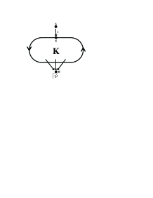
Figure 6:

The most-indicative torrent counterexample to the property $\smash{{\operatorname{{\cal M}}}\models_{{}_{{}_{{\!\!\leq 0.9}}}}{\lozenge{\psi}}}$ is simply $\{\operatorname{GenTorr}(stu)\}$, i.e., a single witness with probability mass 1 associated to the rail $stu$. Although this may seem uninformative, we argue that it is more informative than listing several paths of the form $st\cdots u$ with probability summing up to, say, $0.91$. Our single witness counterexample suggests that the outgoing edge to a state not reaching $\psi$ was simply forgotten; the listing of paths still allows the possibility that one of the probabilities in the whole system is simply wrong.

Nevertheless, if the user needs more information to tackle bugs inside strongly connected components, note that there is more information available at this point. In particular, for every strongly connected component $\operatorname{K}$, every input state $s$ of $\operatorname{K}$ (even for every state in $\operatorname{K}$), and every output state $t$ of $\operatorname{K}$, the probability of reaching $t$ from $s$ is already available from the computation of $\operatorname{Ac}(\operatorname{{\cal M}}_{\psi})$ during the $\operatorname{SCC}$ analysis stage of Section 7.2.

8 Final Discussion

We have presented a novel technique for representing and computing counterexamples for nondeterministic and probabilistic systems. We partition a counterexample in witnesses and state five properties that we believe good witnesses should satisfy in order to be useful as debugging tool: (similarity) elements of a witness should provide similar debugging information; (originality) different witnesses should provide different debugging information; (accuracy) witnesses with higher probability should indicate system behavior more likely to contain errors; (significance) probability of a witness should be relatively high; (finiteness) there should be finitely many witnesses. We achieve this by grouping finite paths in a counterexample together in a witness if they behave the same outside the strongly connected components.

Presently, some work has been done on counterexample generation techniques for different variants of probabilistic models (Discrete Markov chains and Continues Markov chains) [AHL05, AL06, HK07a, HK07b]. In our terminology, these works consider witnesses consisting of a single finite path. We have already discussed in the Introduction that the single path approach does not meet the properties of accuracy, originality, significance, and finiteness.

Instead, our witness/torrent approach provides a high level of abstraction of a counterexample. By grouping together finite paths that behave the same outside strongly connected components in a single witness, we can achieve these properties to a higher extent. Behaving the same outside strongly connected components is a reasonable way of formalizing the concept of providing similar debugging information. This grouping also makes witnesses significantly different form each other: each witness comes form a different rail and each rail provides a different way to reach the undesired property. Then each witness provides original information. Of course, our witnesses are more significant than single finite paths, because they are sets of finite paths. This also gives us more accuracy than the approach with single finite paths, as a collection of finite paths behaving the same and reaching an undesired condition with high probability is more likely to show how the system reaches this condition than just a single path. Finally, because there is a finite number of rails, there is also a finite number of witnesses.

Another key difference of our work to previous ones is that our technique allows us to generate counterexamples for probabilistic systems with nondeterminism. However, a recent report [AL07] also considers counterexample generation for $\operatorname{MDPs}$. This work is limited to upper bounded pCTL formulas without nested temporal operators. Besides, their technique significantly differs from ours.

Finally, among the related work, we would like to stress the result of [HK07a], which provides a systematic characterization of counterexample generation in terms of shortest paths problems. We use this result to generate counterexamples for the acyclic Markov Chains.

In the future we intend to implement a tool to generate our significant diagnostic counterexamples; a very preliminary version has already been implemented. There is still work to be done on improving the visualization of the witnesses, in particular, when a witness captures a large strongly connected component. Another direction is to investigate how this work can be extended to timed systems, either modeled with continuous time Markov chains or with probabilistic timed automata.

Appendix: Proofs

In this appendix we give proofs of the results that were omitted from the paper for space reasons.

Observation 8.1.

Let $\operatorname{{\cal M}}$ be a $\operatorname{MC}$. Since $\operatorname{Ac}(\operatorname{{\cal M}})$ is acyclic we have $\sigma_{i}\not\sim\sigma_{j}$ for every $\sigma\in\operatorname{Paths}^{\star}(\operatorname{Ac}(\operatorname{{\cal M}}))$ and $i\not=j$ (with the exception of absorbing states).

Observation 8.2.

Let $\sigma,\omega$ and $f$ be such that $\sigma\preceq_{f}\omega$. Then $\forall i:\exists j:\omega_{i}\sim\sigma_{j}$. This follows from $\sigma\sqsubseteq_{f}\omega$ and the inertia property.

Lemma 8.3.

Let $\operatorname{{\cal M}}$ be a $\operatorname{MC}$, and $\sigma ts\in\operatorname{Paths}^{\star}(\operatorname{Ac}(\operatorname{{\cal M}}))$. Additionally let $\Delta_{\sigma ts}\triangleq\{\rho\operatorname{tail}(\pi)|\rho\in\operatorname{GenTorr}(\sigma t),\pi\in\operatorname{Paths}^{\star}(\operatorname{SCC}^{+}_{t},t,\{s\})\}$. Then $\Delta_{\sigma ts}=\operatorname{GenTorr}(\sigma ts)$.

Proof.

.

$(\ \supseteq\ )$ Let $\rho_{0}\rho_{1}\cdots\rho_{k}\in\operatorname{GenTorr}(\sigma ts)$ and $n_{t}$ the lowest subindex of $\rho$ such that $\rho_{n_{t}}=t$. Take $\rho\triangleq\rho_{0}\rho_{1}\cdots\rho_{n_{t}}$ and $\pi\triangleq\rho_{n_{t}}\cdots\rho_{k}$ (Note that $\rho_{0}\rho_{1}\cdots\rho_{k}=\rho\operatorname{tail}(\pi)$). In order to prove that $\rho_{0}\rho_{1}\cdots\rho_{k}\in\Delta_{\sigma ts}$ we need to prove that

1. $\rho\in\operatorname{GenTorr}(\sigma t)$, and

2. $\pi\in\operatorname{Paths}^{\star}(\operatorname{SCC}^{+}_{t},t,\{s\})$.

• Let $f$ be such that $\sigma ts\preceq_{f}\rho_{0}\rho_{1}\cdots\rho_{k}$ and $f(|\sigma ts|-1)=k$. Take $g:\{0,1,\ldots,|\sigma t|-1\}\rightarrow\mathbb{N}$ be the restriction of $f$ . It is easy to check that $\sigma t\preceq_{g}\rho$. Additionally $f(|\sigma t|-1)=n_{t}$ (otherwise $f$ would not satisfy the freshness property for $i=|\sigma t|-1$). Then, by definition of $g$, we have $g(|\sigma t|-1)=n_{t}$.

• It is clear that $\pi$ is a path from $t$ to $s$. Therefore we only have to show that every state of $\pi$ is in $\operatorname{SCC}^{+}_{t}$. By definition of $\operatorname{SCC}^{+}_{t}$, $\pi_{0}=t\in\operatorname{SCC}^{+}_{t}$ and $s\in\operatorname{SCC}^{+}_{t}$ since $s\in\operatorname{Out}_{\operatorname{SCC}^{+}_{t}}$. Additionally, since $f$ satisfies inertia property we have that $\forall_{f(|\sigma t|-1)<j<f(|\sigma ts|-1)}:\rho_{f(|\sigma t|-1)}\sim\rho_{j}$, since $f(|\sigma t|-1)=n_{t}$ and $\pi\triangleq\rho_{n_{t}}\cdots\rho_{k}$ we have $\forall_{0<j<|\pi|-1}:t\sim\pi_{j}$ proving that $\pi_{j}\in\operatorname{SCC}^{+}_{t}$ for $j\in\{1,\cdots,|\pi|-2\}$.

$(\ \subseteq\ )$ Take $\rho\in\operatorname{GenTorr}(\sigma t)$ and $\operatorname{tail}(\pi)\in\operatorname{Paths}^{\star}(\operatorname{SCC}^{+}_{t},t,\{s\})$. In order to prove that $\rho\operatorname{tail}(\pi)\in\operatorname{GenTorr}(\sigma ts)$ we need to show that there exists a function $g$ such that:

1. $\sigma ts\preceq_{g}\rho\operatorname{tail}(\pi)$,

2. $g(|\sigma ts|-1)=|\rho\operatorname{tail}(\pi)|-1$.

Since $\rho\in\operatorname{GenTorr}(\sigma t)$ we know that there exists $f$ be such that $\sigma t\preceq_{f}\rho$ and $f(|\sigma t|-1)=|\rho|-1$. We define $g:\{0,1,\ldots,|\sigma ts|-1\}\rightarrow\{0,1,\ldots,|\rho\operatorname{tail}(\pi)|-1\}$ by

$$g(i) \triangleq\left\{\begin{array}[]{ll}f(i)&\mbox{ if }i<|\sigma ts|-1,\\ |\rho\operatorname{tail}(\pi)|-1&\mbox{ if }i=|\sigma ts|-1.\\ \end{array}\right.$$

• It is easy to check that $\sigma ts\sqsubseteq_{g}\rho\operatorname{tail}(\pi)$. Now we will show that $g$ satisfies Freshness and Inertia properties.

  Freshness property: We need to show that for all $0\leq i<|\sigma ts|$ we have $\forall_{0\leq j<g(i)}:\rho\operatorname{tail}(\pi)_{g(i)}\not\sim\rho\operatorname{tail}(\pi)_{j}$. For the cases $i\in\{0,\ldots,|\sigma t|-1\}$ this holds since $\sigma t\preceq_{f}\rho$ and definition of $g$.

  Consider $i=|\sigma ts|-1$, in this case we have to prove $\forall_{0\leq j<|\rho\operatorname{tail}(\pi)|-1}:\rho\operatorname{tail}(\pi)_{|\rho\operatorname{tail}(\pi)|-1)}\not\sim\rho\operatorname{tail}(\pi)_{j}$ or equivalently $\forall_{0\leq j<|\rho\operatorname{tail}(\pi)|-1}:s\not\sim\rho\operatorname{tail}(\pi)_{j}$.

  • Since $\pi\in\operatorname{Paths}^{\star}(\operatorname{SCC}^{+}_{t},t,\{s\})$ and $s\in\operatorname{Out}^{+}_{\operatorname{SCC}^{+}_{t}}$ we have $\forall_{0\leq j<|\operatorname{tail}(\pi)|-1}:s\not\sim\operatorname{tail}(\pi)_{j}$

  • Since $\sigma ts\in\operatorname{Paths}^{\star}(\operatorname{Ac}(\operatorname{{\cal M}}))$ and Observation 8.1 we have $\forall_{0\leq j<|\sigma t|-1}:s\not\sim\sigma t_{j}$. Additionally, $\sigma t\preceq_{f}\rho$, def. $g$, and Observation 8.2 imply $\forall_{0\leq j<|\rho|}:s\not\sim\rho_{j}$ or equivalently $\forall_{0\leq j<|\rho|}:s\not\sim\rho\operatorname{tail}(\pi)_{j}$.

  Inertia property: Since $\pi\in\operatorname{Paths}^{\star}(SCC^{+}_{t},t,\{s\})$ we know that $\forall_{0\leq j<|\pi|-1}:t\sim\pi_{j}$ which implies that $\forall_{|\rho|-1<j<|\rho\operatorname{tail}(\pi)|-1}:\rho\operatorname{tail}(\pi)_{|\rho|-1}\sim\rho\operatorname{tail}(\pi)_{j}$ or equivalently $\forall_{g(|\sigma|-1)<\allowbreak j<\allowbreak g(|\sigma s|-1)}:\rho\operatorname{tail}(\pi)_{g(|\rho|-1)}\sim\rho\operatorname{tail}(\pi)_{j}$ showing that $g$ satisfies the inertia property.

• Follows from the definition of $g$.

∎

Theorem 5.10. Let $\operatorname{{\cal M}}=(S,s_{0},{\cal P},L)$ be a $\operatorname{MC}$. Then for every rail $\sigma\in\operatorname{Paths}^{\star}(\operatorname{Ac}(\operatorname{{\cal M}}))$ we have

$${\mathbf{Pr}}_{{}_{\operatorname{Ac}(\operatorname{{\cal M}})}}({\langle{\sigma}\rangle})={\mathbf{Pr}}_{{}_{\operatorname{{\cal M}}}}({\operatorname{Torr}({\sigma})}).$$

Proof.

By induction on the structure of $\sigma$.

• ${\mathbf{Pr}}_{\operatorname{Ac}(\operatorname{{\cal M}})}({\langle{s_{0}}\rangle})={\mathbf{Pr}}_{\operatorname{Ac}(\operatorname{{\cal M}})}({\operatorname{Paths}(\operatorname{Ac}(\operatorname{{\cal M}}),s_{0})})=1={\mathbf{Pr}}_{\operatorname{{\cal M}}}({\operatorname{Paths}(\operatorname{{\cal M}},s_{0})})={\mathbf{Pr}}_{\operatorname{{\cal M}}}({\operatorname{Torr}({s_{0}})}).$

• Let $t$ be such that $\operatorname{last}(\sigma)=t$. Suppose that $t\in S_{\operatorname{Com}}$. Then

  $$\begin{array}[]{rclr}\hbox to0.0pt{${\mathbf{Pr}}_{\operatorname{Ac}(\operatorname{{\cal M}})}({\langle{\sigma s}\rangle})$\hss}\\ &=&{\mathbf{Pr}}_{\operatorname{Ac}(\operatorname{{\cal M}})}({\langle{\sigma}\rangle})\cdot\operatorname{Ac}({\cal P})(t,s)\\ &=&{\mathbf{Pr}}_{\operatorname{{\cal M}}}({\operatorname{Torr}({\sigma})})\cdot{\cal P}(t,s)&\\ &&&\hbox to0.0pt{\hss$\{\text{Inductive Hypothesis and definition of }{\cal P}\}$}\\ &=&{\mathbf{Pr}}_{\operatorname{{\cal M}}}({\biguplus_{\rho\in\operatorname{GenTorr}(\sigma)}\langle{\rho}\rangle})\cdot{\cal P}(t,s)&\{\text{Lem.~{}}\ref{lem:generators}\}\\ &=&\sum_{\rho\in\operatorname{GenTorr}(\sigma)}{\mathbf{Pr}}_{\operatorname{{\cal M}}}({\langle{\rho}\rangle})\cdot{\mathbf{Pr}}_{\operatorname{{\cal M}}}({\langle{ts}\rangle})\\ &=&\sum_{\rho\in\operatorname{GenTorr}(\sigma)}{\mathbf{Pr}}_{\operatorname{{\cal M}}}({\langle{\rho\operatorname{tail}(ts)}\rangle})&\\ &&&\hbox to0.0pt{\hss$\{\text{Distributivity and }\operatorname{last}(\rho)=t\text{ for all }\rho\in\operatorname{GenTorr}(\sigma)\}$}\\ &=&\sum_{\rho\in\operatorname{GenTorr}(\sigma),\pi\in\operatorname{Paths}(\operatorname{SCC}^{+}_{t},t,\{s\})}{\mathbf{Pr}}_{\operatorname{{\cal M}}}({\langle{\rho\operatorname{tail}(\pi)}\rangle})\\ &=&\sum_{\rho\in\Delta_{\sigma s}}\mu_{{}_{\operatorname{{\cal M}}}}(\langle{\rho}\rangle)&\{\text{Dfn.~{}}\Delta\}\\ &=&\sum_{\rho\in\operatorname{GenTorr}(\sigma s)}\mu_{{}_{\operatorname{{\cal M}}}}(\langle{\rho}\rangle)&\{\text{Lem.~{}}\ref{lem:torrents}\}\\ &=&{\mathbf{Pr}}_{{}_{\operatorname{{\cal M}}}}({\biguplus_{\rho\in\operatorname{GenTorr}(\sigma s)}\langle{\rho}\rangle})\\ &=&{\mathbf{Pr}}_{{}_{\operatorname{{\cal M}}}}({\operatorname{Torr}({\sigma s})})&\{\text{Lem.~{}}\ref{lem:generators}\}\\ \end{array}$$

  Now suppose that $t\in S_{\operatorname{Inp}}$. We denote by $\operatorname{Ac}({\cal P})$ to the probability matrix of $\operatorname{Ac}(\operatorname{{\cal M}})$, then

  $$\begin{array}[]{rclr}\hbox to0.0pt{${\mathbf{Pr}}_{{}_{\operatorname{Ac}(\operatorname{{\cal M}})}}({\langle{\sigma s}\rangle})$\hss}\\ &=&{\mathbf{Pr}}_{{}_{\operatorname{Ac}(\operatorname{{\cal M}})}}({\langle{\sigma}\rangle})\cdot\operatorname{Ac}({\cal P})(t,s)\\ &=&{\mathbf{Pr}}_{{}_{\operatorname{{\cal M}}}}({\operatorname{Torr}({\sigma})})\cdot\operatorname{Ac}({\cal P})(t,s)&\{\text{HI}\}\\ &=&{\mathbf{Pr}}_{{}_{\operatorname{{\cal M}}}}({\biguplus_{\rho\in\operatorname{GenTorr}(\sigma)}\langle{\rho}\rangle})\cdot\operatorname{Ac}({\cal P})(t,s)&\{\text{Lem.~{}\ref{lem:generators}}\}\\ &=&\left(\sum_{\rho\in\operatorname{GenTorr}(\sigma)}{\mathbf{Pr}}_{{}_{\operatorname{{\cal M}}}}({\langle{\rho}\rangle})\right)\cdot\operatorname{Ac}({\cal P})(t,s)\\ &=&\sum_{\rho\in\operatorname{GenTorr}(\sigma)}{\mathbf{Pr}}_{{}_{\operatorname{{\cal M}}}}({\langle{\rho}\rangle})\cdot{\mathbf{Pr}}_{{}_{\operatorname{{\cal M}},t}}({\operatorname{Paths}(\operatorname{SCC}^{+}_{t},t,\{s\})})&\\ &&&\hbox to0.0pt{\hss$\{\text{By definition of }\operatorname{Ac}({\cal P})\text{ and distributivity}\}$}\\ &=&\sum_{\rho\in\operatorname{GenTorr}(\sigma)}{\mathbf{Pr}}_{{}_{\operatorname{{\cal M}}}}({\langle{\rho}\rangle})\cdot\sum_{\pi\in\operatorname{Paths}^{\star}(\operatorname{SCC}^{+}_{t},t,\{s\})}{\mathbf{Pr}}_{{}_{\operatorname{{\cal M}},t}}({\langle{\pi}\rangle})\\ &=&\sum_{\rho\in\operatorname{GenTorr}(\sigma),\pi\in\operatorname{Paths}^{\star}(\operatorname{SCC}^{+}_{t},t,\{s\})}{\mathbf{Pr}}_{{}_{\operatorname{{\cal M}}}}({\langle{\rho\operatorname{tail}(\pi)}\rangle})&\{\text{Dfn.~{}}\mu\}\\ &=&\sum_{\rho\in\Delta_{\sigma s}}{\mathbf{Pr}}_{{}_{\operatorname{{\cal M}}}}({\langle{\rho}\rangle})&\{\text{Dfn.~{}}\Delta\}\\ &=&\sum_{\rho\in\operatorname{GenTorr}(\sigma s)}{\mathbf{Pr}}_{{}_{\operatorname{{\cal M}}}}({\langle{\rho}\rangle})&\{\text{Lem.~{}\ref{lem:torrents}}\}\\ &=&{\mathbf{Pr}}_{{}_{\operatorname{{\cal M}}}}({\biguplus_{\rho\in\operatorname{GenTorr}(\sigma s)}\langle{\rho}\rangle})\\ &=&{\mathbf{Pr}}_{{}_{\operatorname{{\cal M}}}}({\operatorname{Torr}({\sigma s})})&\{\text{Lem.~{}\ref{lem:generators}}\}\\ \end{array}$$

∎

References

- [AHL05] Husain Aljazzar, Holger Hermanns, and Stefan Leue. Counterexamples for timed probabilistic reachability. In Formal Modeling and Analysis of Timed Systems (FORMATS ’05), volume 3829, pages 177–195, 2005.
- [AL06] Husain Aljazzar and Stefan Leue. Extended directed search for probabilistic timed reachability. In Formal Modeling and Analysis of Timed Systems (FORMATS ’06), pages 33–51, 2006.
- [AL07] Husain Aljazzar and Stefan Leue. Counterexamples for model checking of markov decision processes. Computer Science Technical Report soft-08-01, University of Konstanz, December 2007.
- [BdA95] Andrea Bianco and Luca de Alfaro. Model checking of probabilistic and nondeterministic systems. In G. Goos, J. Hartmanis, and J. van Leeuwen, editors, Foundations of Software Technology and Theoretical Computer Science (FSTTCS ’95), volume 1026, pages 499–513, 1995.
- [Bel57] Richard E. Bellman. A Markovian decision process. J. Math. Mech., 6:679–684, 1957.
- [BLR05] Gerd Behrmann, Kim G. Larsen, and Jacob I. Rasmussen. Optimal scheduling using priced timed automata. SIGMETRICS Perform. Eval. Rev., 32(4):34–40, 2005.
- [Cas93] Christos G. Cassandras. Discrete Event Systems: Modeling and Performance Analysis. Richard D. Irwin, Inc., and Aksen Associates, Inc., 1993.
- [CGJ+00] Edmund M. Clarke, Orna Grumberg, Somesh Jha, Yuan Lu, and Helmut Veith. Counterexample-guided abstraction refinement. In Computer Aided Verification, pages 154–169, 2000.
- [dA97] Luca de Alfaro. Formal Verification of Probabilistic Systems. PhD thesis, Stanford University, 1997.
- [dAKM97] Luca de Alfaro, Arjun Kapur, and Zohar Manna. Hybrid diagrams: A deductive-algorithmic approach to hybrid system verification. In Symposium on Theoretical Aspects of Computer Science, pages 153–164, 1997.
- [Epp98] David Eppstein. Finding the k shortest paths. In SIAM Journal of Computing, pages 652–673, 1998.
- [FV97] J. Filar and K. Vrieze. Competitive Markov Decision Processes. 1997.
- [HK07a] Tingting Han and Joost-Pieter Katoen. Counterexamples in probabilistic model checking. In Tools and Algorithms for the Construction and Analysis of Systems: 13th International Conference (TACAS ’07), volume 4424, pages 60–75, 2007.
- [HK07b] Tingting Han and Joost-Pieter Katoen. Providing evidence of likely being on time counterexample generation for ctmc model checking. In International Symposium on Automated Technology for Verification and Analysis (ATVA ’07), volume 4762, pages 331–346, 2007.
- [MP91] Z. Manna and A. Pnueli. The Temporal Logic of Reactive and Concurrent Systems: Specification. Springer, 1991.
- [PZ93] Amir Pnueli and Lenore D. Zuck. Probabilistic verification. Information and Computation, 103(1):1–29, 1993.
- [SdV04] Ana Sokolova and Erik P. de Vink. Probabilistic automata: System types, parallel composition and comparison. In Christel Baier, Boudewijn R. Haverkort, Holger Hermans, Joost-Pieter Katoen, and Markus Siegle, editors, Validation of Stochastic Systems: A Guide to Current Research, volume 2925, pages 1–43. 2004.
- [SL95] Roberto Segala and Nancy Lynch. Probabilistic simulations for probabilistic processes. Nordic Journal of Computing, 2(2):250–273, 1995.
- [Var85] M.Y. Vardi. Automatic verification of probabilistic concurrent finite-state systems. In Proc. 26th IEEE Symp. Found. Comp. Sci., pages 327–338, 1985.