Limit theorems for sample eigenvalues in a generalized spiked population model

Abstract.

In the spiked population model introduced by Johnstone [10], the population covariance matrix has all its eigenvalues equal to unit except for a few fixed eigenvalues (spikes). The question is to quantify the effect of the perturbation caused by the spike eigenvalues. Baik and Silverstein [6] establishes the almost sure limits of the extreme sample eigenvalues associated to the spike eigenvalues when the population and the sample sizes become large. In a recent work [5], we have provided the limiting distributions for these extreme sample eigenvalues. In this paper, we extend this theory to a generalized spiked population model where the base population covariance matrix is arbitrary, instead of the identity matrix as in Johnstone’s case. New mathematical tools are introduced for establishing the almost sure convergence of the sample eigenvalues generated by the spikes.

1. Introduction

Let $(T_{p})$ be a sequence of $p\times p$ non-random and nonnegative definite Hermitian matrices and let $(w_{ij})$, $i,j\geq 1$ be a doubly infinite array of i.i.d. complex-valued random variables satisfying

$$\;\mathbb{E}(w_{11})=0,\leavevmode\nobreak\ \leavevmode\nobreak\ \;\mathbb{E}(|w_{11}|^{2})=1,\leavevmode\nobreak\ \leavevmode\nobreak\ \;\mathbb{E}(|w_{11}|^{4})<\infty.$$

Write $Z_{n}=(w_{ij})_{1\leq i\leq p,1\leq j\leq n}$, the upper-left $p\times n$ bloc, where $p=p(n)$ is related to $n$ such that when $n\rightarrow\infty$, $p/n\rightarrow y>0$. Then the matrix $S_{n}=\frac{1}{n}T_{p}^{1/2}Z_{n}Z_{n}^{*}T_{p}^{1/2}$ can be considered as the sample covariance matrix of an i.i.d. sample $({\bf x}_{1},\ldots,{\bf x}_{n})$ of $p$-dimensional observation vectors ${\bf x}_{j}=T_{p}^{1/2}{{\bf u}_{j}}$ where ${{\bf u}_{j}}=(w_{ij})_{1\leq i\leq p}$ denotes the $j$-th column of $Z_{n}$. Throughout the paper, $A^{1/2}$ stands for any Hermitian square root of an nonnegative definite (n.n.d.) Hermitian matrix $A$.

Assume that the empirical spectral distribution (ESD) of $T_{p}$ converges weakly to a nonrandom probability distribution $H$ on $[0,\infty)$. It is then well-known that the ESD of $S_{n}$ converges to a nonrandom limiting spectral distribution (LSD) $G$ [11, 13].

Let $\lambda_{n,1}\geq\cdots\geq\lambda_{n,p}$ be the set of sample eigenvalues, i.e. the eigenvalues of the sample covariance matrix $S_{n}$. The so-called null case corresponds to the situation $T_{p}\equiv I_{p}$, so that, assuming $y\leq 1$, the LSD $G$ reduces to the Marčenko-Pastur law with support $\Gamma_{G}=[a_{y},b_{y}]$ where $a_{y}=(1-\sqrt{y})^{2}$ and $b_{y}=(1+\sqrt{y})^{2}$. Furthermore, the extreme sample eigenvalues $\lambda_{n,1}$ and $\lambda_{n,p}$ almost surely tend to $b_{y}$ and $a_{y}$, respectively, and the sample eigenvalues $(\lambda_{n,j})$ fill completely the interval $[a_{y},b_{y}]$. However, as pointed out by Johnstone [10], many empirical data sets demonstrate a significant deviation from this null case since some of sample extreme eigenvalues are well separated from an inner bulk interval. As a way for possible explanation of such phenomenon, Johnstone proposes a spiked population model where all eigenvalues of $T_{p}$ are unit except a fixed and relatively small number among them (spikes). In other words, the population eigenvalues $\{\beta_{n,j}\}$ of $T_{p}$ are

$$\underbrace{\alpha_{1},\ldots,\alpha_{1}}_{n_{1}},\ldots,\underbrace{\alpha_{K},\ldots,\alpha_{K}}_{n_{K}},\underbrace{1,\ldots,1}_{p-M},$$

where $M$ is fixed as well as the multiplicity numbers $(n_{k})$ which satisfy $n_{1}+\cdots+n_{K}=M$. Clearly, this spiked population model can be viewed as a finite-rank perturbation of the null case.

Obviously, the LSD $G$ of $S_{n}$ is not affected by this small perturbation, still equals to the Marčenko-Pastur law. However, the asymptotic behavior of the extreme eigenvalues of $S_{n}$ is significantly different from the null case. The fluctuation of the largest eigenvalue $\lambda_{n,1}$ in case of complex Gaussian variables has been recently studied in Baik et al. [7]. These authors prove a transition phenomenon: the weak limit as well as the scaling of $\lambda_{n,1}$ is different according to its location with respect to a critical value $1+\sqrt{y}$. In Baik and Silverstein [6], the authors consider the spiked population model with general random variables: complex or real and not necessarily Gaussian. For the almost sure limits of the extreme sample eigenvalues, they also find that these limits depend on the critical values $1+\sqrt{y}$ for largest sample eigenvalues, and on $1-\sqrt{y}$ for smallest ones. For example, if there are $m$ eigenvalues in the population covariance matrix larger than $1+\sqrt{y}$, then the $m$ largest sample eigenvalues $\lambda_{n,1},\ldots,\lambda_{n,m}$ will converge to a limit above the right edge $b_{y}$ of the limiting Marčenko-Pastur law, see §4.1 for more details. In a recent work Bai and Yao [5], considering general random matrices as in [6], we have established central limit theorems for these extreme sample eigenvalues generated by spike eigenvalues which are outside the critical interval $[1-\sqrt{y},1+\sqrt{y}]$.

The spiked population model has also an extension to other random matrices ensembles through the general concept of small-rank perturbations. The goal is again to examine the effect caused on the sample extreme eigenvalues by such perturbations. In a series of recent papers [12, 9, 8], these authors establish several results in this vein for ensembles of form $M_{n}=W_{n}+n^{-1/2}V$ where $W_{n}$ is a standard Wigner matrix and $V$ a small-rank matrix.

The present work is motivated by a generalization of Johnstone’s spike population model defined as follows. The population covariance matrix $T_{p}$ posses two sets of eigenvalues: a small number of them, say $(\alpha_{k})$, called generalized spikes, are well separated - in a sense to be defined later-, from a base set $(\beta_{n,i})$. In other words, the spectrum of $T_{p}$ reads as

$$\underbrace{\alpha_{1},\ldots,\alpha_{1}}_{n_{1}},\ldots,\underbrace{\alpha_{K},\ldots,\alpha_{K}}_{n_{K}},\beta_{n,1},\ldots,\beta_{n,p-M}.$$

Therefore, this scheme can be viewed as a finite-rank perturbation of a general population covariance matrix with eigenvalues $\{\beta_{n,j}\}$.

The empirical distributions generated by the eigenvalues $(\beta_{n,i})$ will be assumed to have a limit distribution $H$. Note that $H$ is also the LSD of $T_{p}$ since the perturbation is of finite rank. Analogous to Johnstone’s spiked population model, the LSD $G$ of the sample covariance matrix $S_{n}$ is still not affected by the spikes. The aim of this work is to identify the effect caused by the spikes $(\alpha_{k})$ on a particular subset of sample eigenvalues. The results obtained here extend those of [6, 5] to the present generalized scheme.

The remaining sections of the paper are organized as following. §2 gives the precise definition of the generalized spiked population model. Next, we use §3 to recall several useful results on the convergence of the E.S.D. from general sample covariance matrices. In §4, we examine the strong point-wise convergence of sample eigenvalues associated to spikes. We then establish CLT for these sample eigenvalues in §5 using the methodology developed in [5]. Preliminary lemmas and their proofs are gathered in the last section.

2. Generalized spiked population model

In a generalized spiked population model, the population covariance matrix $T_{p}$ takes the form

$$T_{p}=\begin{pmatrix}\Sigma&0\\ 0&V_{p}\end{pmatrix},$$

where $\Sigma$ and $V_{p}$ are nonnegative and nonrandom Hermitian matrices of dimension $M\times M$ and $p^{\prime}\times p^{\prime}$, respectively, where $p^{\prime}=p-M$. The submatrix $\Sigma$ has $K$ eigenvalues $\alpha_{1}>\cdots>\alpha_{K}>0$ of respective multiplicity $(n_{k})$, and $V_{p}$ has $p^{\prime}$ eigenvalues $\beta_{n,1}\geq\cdots\geq\beta_{n,p^{\prime}}$.

Throughout the paper, we assume that the following assumptions hold.

1. $w_{ij}$, $i,j=1,2,...$ are i.i.d. complex random variables with $Ew_{11}=0$, $E|w_{11}|^{2}=1$, and $E|w_{11}|^{4}<\infty$.

2. $n=n(p)$ with $y_{n}=p^{\prime}/n\to y>0$ as $n\to\infty$.

3. The sequence of ESD $H_{n}$ of $(T_{p})$, i.e. generated by the population eigenvalues $\{\alpha_{k},\beta_{n,j}\}$, weakly converges to a probability distribution $H$ as $n\to\infty$.

4. The sequence $(\|T_{p}\|)$ of spectral norms of $(T_{p})$ is bounded.

For any measure $\mu$ on $\mathbb{R}$, we denote by $\Gamma_{\mu}$ the support of $\mu$, a close set.

Definition 2.1.

An eigenvalue $\alpha$ of the matrix $\Sigma$ is called a generalized spike eigenvalue if $\alpha\notin\Gamma_{H}$.

To avoid confusion between spikes and non-spike eigenvalues, we further assume that

1. $\max\limits_{1\leq j\leq p^{\prime}}d(\beta_{nj},\Gamma_{H})=\varepsilon_{n}\to 0$,

where $d(x,A)$ denotes the distance of a point $x$ to a set $A$. Note that there is a positive constant $\delta$ such that $d(\alpha_{k},\Gamma_{H})>\delta$, for all $k\leq K$.

The above definition for generalized spikes is consistent with Johnstone’s original one of (ordinary) spikes, since in that case we have $H_{n}\equiv H=\delta_{\{1\}}$ and $\alpha\notin\Gamma_{H}$ simply means $\alpha\neq 1$.

Let us decompose the observation vectors ${\bf x}_{j}=T_{p}^{1/2}{{\bf u}_{j}}$, $j=1,\ldots,n$, where ${{\bf u}_{j}}=(w_{ij})_{1\leq i\leq p}$ by blocs,

$${\bf x}_{j}=\begin{pmatrix}{\mbox{\boldmath$\xi$}}_{j}\\ {\mbox{\boldmath$\eta$}}_{j}\end{pmatrix},\quad\textrm{with}\quad{\mbox{\boldmath$\xi$}}_{j}=\Sigma^{1/2}(w_{ij})_{1\leq i\leq M},\quad{\mbox{\boldmath$\eta$}}_{j}=V_{p}^{1/2}(w_{ij})_{M<i\leq p}.$$

Note that both sequences $\{{\mbox{\boldmath$\xi$}}_{1},\ldots,{\mbox{\boldmath$\xi$}}_{n}\}$ and $\{{\mbox{\boldmath$\eta$}}_{1},\ldots,{\mbox{\boldmath$\eta$}}_{n}\}$ are i.i.d. sequences. We also denote the coordinates of ${\mbox{\boldmath$\xi$}}_{1}$ by ${\mbox{\boldmath$\xi$}}_{1}=(\xi(1),\ldots,\xi(M))^{T}$.

Similarly, the sample covariance matrix $S_{n}=\frac{1}{n}T_{p}^{1/2}Z_{n}Z_{n}^{*}T_{p}^{1/2}$ is decomposed as

$$S_{n}=\begin{pmatrix}S_{11}&S_{12}\\ S_{21}&S_{22}\end{pmatrix}=\begin{pmatrix}X_{1}X_{1}^{*}&X_{1}X_{2}^{*}\\ X_{2}X_{1}^{*}&X_{2}X_{2}^{*}\end{pmatrix}\leavevmode\nobreak\ ,$$

with

$$X_{1}=\frac{1}{\sqrt{n}}({\mbox{\boldmath$\xi$}}_{1},\cdots,{\mbox{\boldmath$\xi$}}_{n})_{M\times n}=\frac{1}{\sqrt{n}}{\mbox{\boldmath$\xi$}}_{1:n},\ X_{2}=\frac{1}{\sqrt{n}}({\mbox{\boldmath$\eta$}}_{1},\cdots,{\mbox{\boldmath$\eta$}}_{n})_{p^{\prime}\times n}=\frac{1}{\sqrt{n}}{\mbox{\boldmath$\eta$}}_{1:n}\leavevmode\nobreak\ .$$

Throughout the paper and for any Hermitian matrix $A$, we order its eigenvalues in an descending order as $\lambda_{1}^{A}\geq\lambda_{2}^{A}\geq\cdots.$ By definition, the sample eigenvalues $\{\lambda^{S_{n}}_{j},1\leq j\leq p\}$ are solutions to the equation

(2.1) $$0=|\lambda I-S_{n}|=|\lambda I-S_{22}|\leavevmode\nobreak\ |\lambda I-K_{n}(\lambda)|\leavevmode\nobreak\ ,$$

with a random sesquilinear form

(2.2) $$K_{n}(\lambda)=S_{11}+S_{12}(\lambda I-S_{22})^{-1}S_{21}.$$

Note that the factorization (2.1) holds for any $\lambda\notin\mathop{\textrm{spec}}(S_{22})$. This identity will play a central role in our analysis.

3. Known results on the spectrum of large sample covariance matrices

3.1. Marčenko-Pastur distributions

In this section $y$ is an arbitrary positive constant and $H$ an arbitrary probability measure on $\mathbb{R}^{+}$. Define on the set

$$\mathbb{C}^{+}:=\{z\in\mathbb{C}\leavevmode\nobreak\ :\leavevmode\nobreak\ \Im(z)>0\leavevmode\nobreak\ \}\leavevmode\nobreak\ ,$$

the map

(3.1) $$g(s)=g_{y,H}(s)=-\frac{1}{s}+y\int\!\frac{t}{1+ts}dH(t)\leavevmode\nobreak\ ,\quad s\in\mathbb{C}^{+}.$$

It is well-known ([4, Chap. 5]) that $g$ is a one-to-one map from $\mathbb{C}^{+}$ onto itself, and the inverse map $m=g^{-1}$ corresponds to the Stieltjies transform of a probability measure $F_{y,H}$ on $[0,\infty)$. Throughout the paper and with a small abuse of language, we refer $F_{y,H}$ as the Marčenko-Pastur (M.P.) distribution with indexes $(y,H)$.

This family of distributions arises naturally as follows. Consider a companion matrix ${\underline{S}}_{n}=\frac{1}{n}Z_{n}^{*}T_{p}Z_{n}$ of the sample covariance matrix $S_{n}$. The spectra of $S_{n}$ and ${\underline{S}}_{n}$ are identical except $|n-p|$ zeros. It is then well-known ([11],[4, Chap. 5]) that under Conditions (a)-(d), the E.S.D. of ${\underline{S}}_{n}$ converges to the M.P. distribution $F_{y,H}$. The terminology is slightly ambiguous since the classical M.P. distribution refers to the limit of the E.S.D. of $S_{n}$ when $T_{p}=I_{p}$.

Note that we shall always extend a function $h$ defined on $\mathbb{C}^{+}$ to the real axis $\mathbb{R}$ by taking the limits $\lim_{\varepsilon\to 0_{+}}h(x+i\varepsilon)$ for real $x$’s whenever these limits exist. For $\alpha\notin\Gamma_{H}$ and $\alpha\neq 0$ define

(3.2) $$\psi(\alpha)=\psi_{y,H}(\alpha):=g(-1/\alpha)=\alpha+y\alpha\int\!\frac{t}{\alpha-t}dH(t)\leavevmode\nobreak\ .$$

Note that even though this formula could be extended to $\alpha=0$ when $0\notin\Gamma_{H}$, as we will see below that $\alpha$ is related to the $-1/m$ where $m$ is a Stieltjies transform, so that there is no much meaning for $\alpha=0$. Therefore, the point 0 will always be excluded from the domain of definition of $\psi$.

Analytical properties of $F_{y,H}$ can be derived from the fundamental equation (3.2). The following lemma, due to Silverstein and Choi [14], characterizes the close relationship between the supports of the generating measure $H$ and the generated M.P. distribution $F_{y,H}$.

Lemma 3.1.

If $\lambda\notin\Gamma_{F_{y,H}}$, then $m(\lambda)\neq 0$ and $\alpha=-1/m(\lambda)$ satisfies

1. $\alpha\notin\Gamma_{H}$ and $\alpha\neq 0$ (so that $\psi(\alpha)$ is well-defined);

2. $\psi^{\prime}(\alpha)>0$.

Conversely, if $\alpha$ satisfies (i)-(ii), then $\lambda=\psi(\alpha)\notin\Gamma_{F_{y,H}}$.

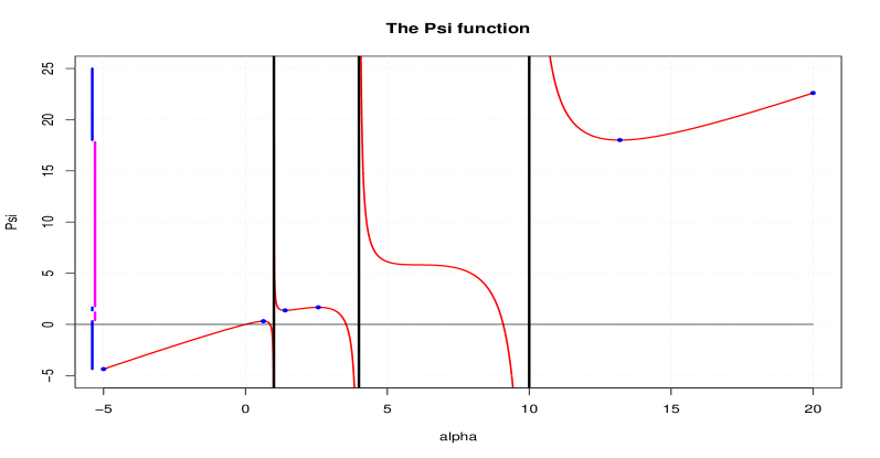
Figure 1. The $\psi$ function for the Marčenko-Pastur distribution $F_{0.3,H}$ with $H$ the uniform distribution on the set $\{1,4,10\}$. Blue points indicate intervals where $\psi^{\prime}>0$. Singular points of $\psi$ are indicated as vertical lines corresponding to the support of $H$. On the left, the support set of $F_{0.3,H}$ (except the point 0) and its complementary set are indicated as magenta and blue segments respectively.

It is then possible to determine the support of $F_{y,H}$ by looking at intervals where $\psi^{\prime}>0$. As an example, Figure 1 displays the function $\psi$ for the M.P. distribution with indexes $y=0.3$ and $H$ the uniform distribution on the set $\{1,4,10\}$. The function $\psi$ is strictly increasing on the following intervals: ($-\infty$, 0), (0, 0.63), (1.40, 2.57) and (13.19, $\infty$). According to Lemma 3.1, we get

$$\Gamma_{F_{y,H}}\cap\mathbb{R}^{*}=(0,\leavevmode\nobreak\ 0.32)\cup(1.37,\leavevmode\nobreak\ 1.67)\cup(18.00,\leavevmode\nobreak\ \infty).$$

Hence, taking into account that 0 belongs to the support of $F_{y,H}$, we have

$$\Gamma_{F_{y,H}}=\{0\}\cup[0.32,\leavevmode\nobreak\ 1.37]\cup[1.67,\leavevmode\nobreak\ 18.00].$$

We refer to Bai and Silverstein [3] for a complete account of analytical properties of the family of M.P. distributions $\{F_{y,H}\}$ and the maps $\{\psi_{y,H}\}$. In particular, the following conclusions will be useful:

• when restricted to $\Gamma^{c}_{F_{y,H}}$, $\psi_{y,H}$ has a well-defined inverse function $\psi^{-1}_{y,H}$: $\Gamma^{c}_{F_{y,H}}\to\Gamma^{c}_{H}$ which is strictly increasing;

• the family $\{F_{y,H}\}$ is continuous in its index parameters $(y,H)$ in a wide sense. For example, $\{\psi_{y,H}\}$ tends to the identity function as $y\to 0$.

3.2. Exact separation of sample eigenvalues

We need first quote two results of Bai and Silverstein [2, 3] on exact separation of sample eigenvalues. Recall the ESD’s $(H_{n})$ of $(T_{p})$, $y_{n}=p/n$, and let $\{F_{y_{n},H_{n}}\}$ be the sequence of associated M.P. distributions. One should not confuse the M.P. distribution $\{F_{y_{n},H_{n}}\}$ with the E.S.D. of ${\underline{S}}_{n}$ although both converge to the M.P. distribution $F_{y,H}$ as $n\rightarrow\infty$.

Proposition 3.1.

Assume hold Conditions (a)-(d) and the following

1. The interval $[a,b]$ with $a>0$ lies in an open interval $(c,d)$ outside the support of $F_{y_{n},H_{n}}$ for all large $n$.

Then

$$P(\mbox{ no eigenvalue of $S_{n}$ appears in $[a,b]$ for all large $n$ })=1.$$

Roughly speaking, Proposition 3.1 states that a gap in the spectra of the $F_{y_{n},H_{n}}$’s is also a gap in the spectrum of $S_{n}$ for large $n$. Moreover, under Condition (f), we know by Lemma 3.1, that for large $n$,

$$\psi_{y_{n},H_{n}}^{-1}\{[a,b]\}\subset\psi_{y_{n},H_{n}}^{-1}\{(c,d)\}\subset\Gamma^{c}_{H_{n}}\leavevmode\nobreak\ .$$

By continuity of $F_{y_{n},H_{n}}$ in its indexes, it follows that we have for large $n$

$$\psi^{-1}\{[a,b]\}=\psi_{y,H}^{-1}\{[a,b]\}\subset\Gamma^{c}_{H_{n}}\leavevmode\nobreak\ .$$

In other words, it holds almost surely and for large $n$ that, $\psi^{-1}\{[a,b]\}$ contains no eigenvalue of $T_{p}$. Let for these $n$, the integer $i_{n}\geq 0$ be such that

(3.3) $$\textrm{$T_{p}$ has exactly $i_{n}$ eigenvalues larger than }\psi^{-1}(b)\leavevmode\nobreak\ .$$

Proposition 3.2.

Assume Conditions (a)-(d) and (f) hold. If $y[1-H(0)]\leq 1$, or $y[1-H(0)]>1$ but $[a,b]$ is not contained in $[0,x_{0}]$ where $x_{0}>0$ is the smallest value of the support of $F_{y,H}$, then with $i_{n}$ defined in (3.3) we have

$$P(\lambda_{i_{n}+1}^{S_{n}}\leq a<b\leq\lambda_{i_{n}}^{S_{n}}\quad\mbox{for all large $n$})=1.$$

In other words, under these conditions, it happens eventually that the numbers of sample eigenvalues $\{\lambda_{i}^{S_{n}}\}$ in both sides of $[a,b]$ match exactly the numbers of populations eigenvalues $\{\alpha_{k},\beta_{n,j}\}$ in both sides of the interval $\psi^{-1}\{[a,b]\}$.

4. Almost sure convergence of sample eigenvalues from generalized spikes

From (3.2), we have

$$\psi^{\prime}(\alpha)=1-y\int\!\frac{t^{2}}{(\alpha-t)^{2}}dH(t)\leavevmode\nobreak\ ,\qquad\psi^{\prime\prime\prime}(\alpha)=-6y\int\!\frac{t^{2}}{(\alpha-t)^{4}}dH(t)\leavevmode\nobreak\ .$$

Therefore, when $\alpha$ approaches the boundary of the support of $H$, $\psi^{\prime}(\alpha)$ tends to $-\infty$, see also Figure 1. Moreover, $\psi^{\prime}$ is concave on any interval outside $\Gamma_{H}$.

As we will see, the asymptotic behavior of the sample eigenvalues generated by a generalized spike eigenvalue $\alpha$ depends on the sign of $\psi^{\prime}(\alpha)$.

Definition 4.1.

We call a generalized spike eigenvalue $\alpha$, a distant spike for the M.P. law $F_{y,H}$ if $\psi^{\prime}(\alpha)>0$, and a close spike if $\psi^{\prime}(\alpha)\leq 0$.

Recall that $\psi$ depend on the parameters $(y,H)$. When $H$ is fixed, and since $\psi$ tends to the identity function as $y\to 0$, a close spike for a given M.P. law $F_{y,H}$ becomes a distant spike for M.P. law $F_{y,H}$ for small enough $y$.

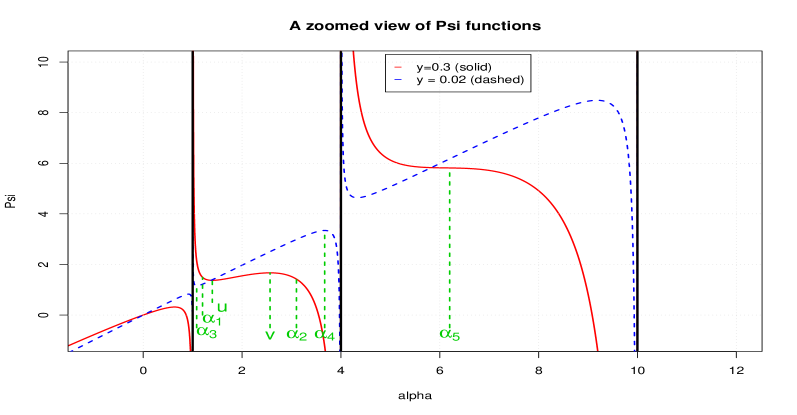
Figure 2. A zoomed view of the $\psi$ functions for the Marčenko-Pastur distribution $F_{0.3,H}$ (solid curve) and $F_{0.02,H}$ (dashed curve) with $H$ the uniform distribution on the set $\{1,4,10\}$. The three points $\alpha_{1}$, $\alpha_{2}$ and $\alpha_{5}$ are close spikes for $F_{0.3,H}$ where $\psi_{0.3,H}^{\prime}\leq 0$. They become all distant spikes for $F_{0.02,H}$ as $\psi_{0.02,H}^{\prime}>0$.

As an example, different types of spikes are displayed in Figure 2. The solid curve corresponds to a zoomed view of $\psi_{0.3,H}$ of Figure 1. For $F_{0.3,H}$, the three values $\alpha_{1}$, $\alpha_{2}$ and $\alpha_{5}$ are close spikes; each small enough $\alpha$ (close to zero), or large enough $\alpha$ (not displayed), or a value between $u$ and $v$ (see the figure) is a distant spike. Furthermore, as $y$ decreases from $0.3$ to $0.02$ (dashed curve), $\alpha_{1}$, $\alpha_{2}$ and $\alpha_{5}$ become all distant spikes.

Throughout this section, for each spike eigenvalue $\alpha_{k}$, we denote by $\nu_{k}+1,\ldots,\nu_{k}+n_{k}$ the descending ranks of $\alpha_{k}$ among the eigenvalues of $T_{p}$ (multiplicities of eigenvalues are counted): in other words, there are $\nu_{k}$ eigenvalues of $T_{p}$ larger than $\alpha_{k}$ and $p-\nu_{k}-n_{k}$ less.

Theorem 4.1.

Assume that the conditions (a)-(e) hold. Let $\alpha_{k}$ be a generalized spike eigenvalue of multiplicity $n_{k}$ satisfying $\psi^{\prime}(\alpha_{k})>0$ (distant spike) with descending ranks $\nu_{k}+1,\cdots,\nu_{k}+n_{k}$. Then, the $n_{k}$ consecutive sample eigenvalues $\{\lambda^{S_{n}}_{i}\}$, $i=\nu_{k}+1,\ldots,\nu_{k}+n_{k}$ converge almost surely to $\psi(\alpha_{k})$.

Proof.

Recall Figure 2 of the $\psi$ function, for each distant spike $\alpha_{k}$, there is an interval $(u_{k},v_{k})$ such that

• $u_{k}<\alpha_{k}<v_{k}$;

• $\psi^{\prime}(u_{k})=\psi^{\prime}(v_{k})=0$;

• $\psi^{\prime}(\alpha)>0$ for all $\alpha\in(u_{k},v_{k})$.

Here we make the convention that $v_{k}=\infty$ if $\psi^{\prime}(\alpha)>0$ for all $\alpha>\alpha_{k}$ and $u_{k}=0$ if $\psi^{\prime}(\alpha)>0$ for all $\alpha\in(0,\alpha_{k})$.

Recall that the support of $F_{y_{n},H_{n}}$ is determined by

(4.1) $$\psi_{n}^{\prime}(\alpha)=\psi_{y_{n},H_{n}}^{\prime}(\alpha)=1-y_{n}\bigg{[}\frac{p^{\prime}}{p}\int\!\frac{t^{2}}{(\alpha-t)^{2}}dH_{n}^{v}(t)\leavevmode\nobreak\ +\frac{1}{p}\sum_{j=1}^{K}\frac{n_{j}\alpha_{j}^{2}}{(\alpha-\alpha_{j})^{2}}\bigg{]},$$

where $H_{n}^{v}=\frac{1}{p^{\prime}}\sum_{j}\delta_{\beta_{n,j}}$ is the ESD of $V_{p}$.

Let $\tilde{v}_{k}=\min(v_{k},\alpha_{k-1})$ if $k>1$ and $\tilde{v}_{k}=v_{k}$ otherwise. Choose $v,v^{\prime}$ and $\alpha^{\prime}_{u},\alpha_{u}$ such that $\alpha_{k}<\alpha^{\prime}_{u}<\alpha_{u}<v<v^{\prime}<\tilde{v}_{k}$. By condition (e), all eigenvalues of $T_{p}$ will keep away from the interval $(\alpha_{u}^{\prime},v^{\prime})$ for all large $n$. Thus, $\psi_{n}^{\prime}(\alpha)\to\psi^{\prime}(\alpha)>0$ uniformly on the interval $[\alpha_{u}^{\prime},v^{\prime}]$. Hence, the interval $(\psi(\alpha_{u}^{\prime}),\psi(v^{\prime}))$ will be out of the support of $F_{y_{n},H_{n}}$ for all large $n$. Consequently, the interval $[\psi(\alpha_{u}),\psi(v)]$ satisfies the conditions of Proposition 3.2 with $i_{n}=\nu_{k}$. Therefore, by Proposition 3.2, we have

$$\begin{cases}P(\lambda_{\nu_{k}+1}^{S_{n}}\leq\psi(\alpha_{u})<\psi(v)\leq\lambda_{\nu_{k}}^{S_{n}},\leavevmode\nobreak\ \mbox{ for all large $n$})=1&\mbox{ if }\nu_{k}>0;\cr P(\lambda_{\nu_{k}+1}^{S_{n}}\leq\psi(\alpha_{u}),\ \mbox{ for all large $n$})=1&\mbox{ otherwise. }\cr\end{cases}$$

Therefore, it holds almost surely

$$\limsup_{n}\lambda_{\nu_{k}+1}^{S_{n}}\leq\psi(\alpha_{u}),$$

and finally, letting $\alpha_{u}\rightarrow\alpha_{k}$,

(4.2) $$\limsup_{n}\lambda_{\nu_{k}+1}^{S_{n}}\leq\psi(\alpha_{k}).$$

Similarly, one can prove that for any $\tilde{u}_{k}<u<\alpha_{l}<\alpha_{k}$,

$$\begin{cases}P(\lambda_{\nu_{k}+n_{k}+1}^{S_{n}}\leq\psi(u)<\psi(\alpha_{l})\leq\lambda_{\nu_{k}+n_{k}}^{S_{n}},\ \mbox{ for all large $n$})=1&\mbox{ if }\nu_{k}+n_{k}<p,\cr P(\lambda_{\nu_{k}+n_{k}}^{S_{n}}\geq\psi(\alpha_{l}),\ \mbox{ for all large $n$})=1&\mbox{ otherwise,}\end{cases}$$

where $\tilde{u}_{k}=\max(u_{k},\alpha_{k+1})$ if $k<K$ and $\tilde{u}_{k}=u_{k}$ otherwise.

Consequently,

(4.3) $$\liminf_{n}\lambda_{\nu_{k}+n_{k}}^{S_{n}}\geq\psi(\alpha_{k}).$$

Thus, we proved that almost surely,

$$\lim_{n}\lambda_{\nu_{k}+j}^{S_{n}}=\psi(\alpha_{k}),\mbox{ for }j=1,\cdots,n_{k}.$$

The proof of Theorem 4.1 is complete. ∎

Next we consider close spikes.

Theorem 4.2.

Assume that the conditions (a)-(e) hold. Let $\alpha_{k}$ be a generalized spike eigenvalue of multiplicity $n_{k}$ satisfying $\psi^{\prime}(\alpha_{k})\leq 0$ (close spike) with descending ranks $\nu_{k}+1,\ldots,\nu_{k}+n_{k}$. Let $I$ be the maximal interval in $\Gamma^{c}_{H}$ containing $\alpha_{k}$.

1. If $I$ has a sub-interval $(u_{k},v_{k})$ on which $\psi^{\prime}>0$ (then we take this interval to be maximal), then the $n_{k}$ sample eigenvalues $\{\lambda^{S_{n}}_{j}\}$, $j=\nu_{k}+1,\ldots,\nu_{k}+n_{k}$ converge almost surely to the number $\psi(w)$ where $w$ is one of the endpoints $\{u_{k},v_{k}\}$ nearest to $\alpha_{k}$ ;

2. If for all $\alpha\in I$, $\psi^{\prime}(\alpha)\leq 0$, then the $n_{k}$ sample eigenvalues $\{\lambda^{S_{n}}_{j}\}$, $j=\nu_{k}+1,\ldots,\nu_{k}+n_{k}$ converge almost surely to the $\gamma$-th quantile of $G$, the L.S.D. of $S_{n}$, where $\gamma=H(0,\alpha_{k})$.

Proof.

The proof refers to the curves of Figure 2.

(i). Suppose $\alpha_{k}$ is a spike eigenvalue satisfying $\psi^{\prime}(\alpha_{k})\leq 0$ and there is an interval $(u_{k},v_{k})\subset I$ on which $\psi^{\prime}>0$ ($\alpha_{k}$ is like the $\alpha_{1}$ on the figure). According to Lemma 3.1, $\psi\{(u_{k},v_{k})\}\subset\Gamma^{c}_{F_{y,H}}$ and $\psi(u_{k})$ is a boundary point of the support of $G$, the L.S.D. of $S_{n}$. Without loss of generality, we can assume $\alpha_{k}\leq u_{k}$, the argument of the other situation where $\alpha_{k}>v_{k}$ being similar.

Choose $u_{k}<\alpha_{u}<v<\tilde{v}$ ($\tilde{v}=\min(v_{k},\alpha_{k-1})$ or $v_{k}$ in accordance with $k>1$ or not) such that $(\alpha_{u},v)\subset I$, by the argument used in the proof of Theorem 4.1, one can prove that

$$\begin{cases}P(\lambda_{\nu_{k}+1}^{S_{n}}\leq\psi(\alpha_{u})<\psi(v)\leq\lambda_{\nu_{k}}^{S_{n}},\leavevmode\nobreak\ \mbox{ for all large $n$})=1&\mbox{ if }\nu_{k}>0;\cr P(\lambda_{\nu_{k}+1}^{S_{n}}\leq\psi(\alpha_{u}),\ \mbox{ for all large $n$})=1&\mbox{ otherwise. }\cr\end{cases}$$

This proves that almost surely,

$$\limsup\lambda_{\nu_{k}+1}^{S_{n}}\leq\psi(u_{k})\leq\liminf\lambda_{\nu_{k}}^{S_{n}}\leavevmode\nobreak\ .$$

On the other hand, since $\psi(u_{k})$ is a boundary point of the support of $G$, we know that for any $\varepsilon>0$, almost surely, the number of $\lambda_{i}^{S_{n}}$’s falling into $[\psi(u_{k})-\varepsilon,\psi(u_{k})]$ tends to infinity. Therefore,

$$\liminf\lambda_{\nu_{k}+n_{k}+1}^{S_{n}}\geq\psi(u_{k})-\varepsilon,\quad\textrm{a.s.}.$$

Since $\varepsilon$ is arbitrary, we have finally proved that almost surely,

$$\lim\lambda_{\nu_{k}+j}^{S_{n}}=\psi(u_{k}),\quad j=1,\cdots,n_{k}.$$

Thus, the proof of Conclusion (i) of Theorem 4.2 is complete.

Similarly, if the spiked eigenvalue $\alpha_{k}$ is like $\alpha_{2}$, we can show that the $n_{k}$ corresponding eigenvalues of $S_{n}$ goes to $\psi(v_{k})$.

(ii)  If the spiked eigenvalues is like $\alpha_{5}$, where the gap of support of LSD disappeared, clearly the corresponding sample eigenvalues $\lambda_{\nu_{k}+1},\ldots,\lambda_{\nu_{k}+n_{k}}$ tend to the $\gamma$-th quantile of the LSD of $S_{n}$ where

$$\gamma=1-\lim\frac{i_{n}}{\nu_{k}}=H(0,\alpha_{k}).$$

∎

4.1. Case of Johnstone’s spiked population model

In the case of Johnstone’s model, $H$ reduces to the Dirac mass $\delta_{1}$ and the LSD $G$ equals the Marčenko-Pastur law with $\Gamma_{G}=[a_{y},b_{y}]$. Each $\alpha>0$, $\alpha\neq 1$ is then a spike eigenvalue. The associated function $\psi$ in (3.2) becomes

(4.4) $$\psi(\alpha_{k})=\alpha_{k}+\frac{y\alpha_{k}}{\alpha_{k}-1}.$$

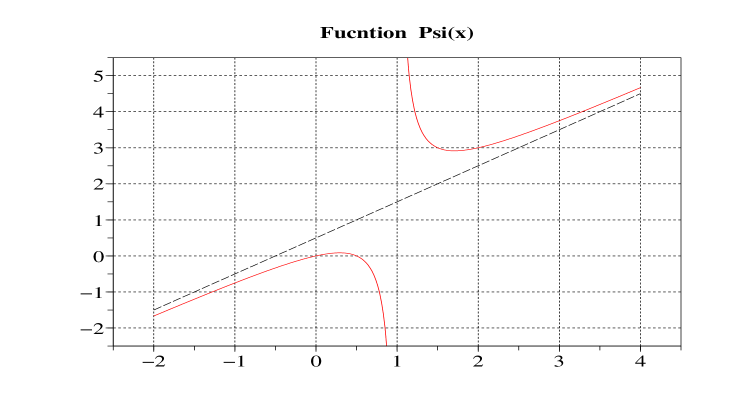
Figure 3. The function $\alpha\mapsto\psi(\alpha)=\alpha+y\alpha/(\alpha-1)$ which maps a spike eigenvalue $\alpha$ to the limit of an associated sample eigenvalue in Johnstone’s spiked population model. Figure with $y=\frac{1}{2}$;  $[1\mp\sqrt{y}]=[0.293,\leavevmode\nobreak\ 1.707]$; $[(1\mp\sqrt{y})^{2}]=[0.086,\leavevmode\nobreak\ 2.914]$ .

The function $\psi$ has the following properties, see Figure 3:

• its range equals $(-\infty,a_{y}]\cup[b_{y},\infty)$ ;

• $\psi(1-\sqrt{y})=a_{y}$ ,  $\psi(1+\sqrt{y})=b_{y}$;

• $\psi^{\prime}(\alpha)>0\Leftrightarrow|\alpha-1|>\sqrt{y}$.

Therefore, by Theorem 4.1, for any spike eigenvalue satisfying $\alpha_{k}>1+\sqrt{y}$ (large enough) or $\alpha_{k}<1-\sqrt{y}$ (small enough), there is a packet of $n_{k}$ consecutive eigenvalues $\{\lambda_{n,j}\}$ converging almost surely to $\psi(\alpha_{k})\notin[a_{y},b_{y}]$. In other words, assume there are exactly $K_{1}$ spikes greater than $1+\sqrt{y}$ and $K_{2}$ spikes smaller than $1-\sqrt{y}$. By Theorems 4.1 and 4.2 we conclude that

1. the $N_{1}:=n_{1}+\ldots+n_{K_{1}}$ largest eigenvalues $\{\lambda_{j}^{S_{n}}\}$, $j=1,\ldots,N_{1}$ tend to their respective limits $\{\psi(\alpha_{k})\}$, $k=1,\ldots,K_{1}$ ;

2. the immediately following largest eigenvalue $\lambda_{N_{1}+1}^{S_{n}}$ tends to the right edge $b_{y}$;

3. the $N_{2}:=n_{K}+\cdots+n_{K-K_{2}+1}$ smallest sample eigenvalues $\{\lambda_{n,p-j}^{S_{n}}\}$, $j=0,\ldots,N_{2}-1$ tend to their respective limits $\{\psi(\alpha_{k})\}$, $k=K,\ldots,K-K_{2}+1$ ;

4. the immediately following smallest eigenvalue $\lambda_{p-N_{2}}^{S_{n}}$ tends to the left edge $a_{y}$.

Hence we have recovered the content of Theorem 1.1 of [6].

4.2. An example of generalized spike eigenvalues

Assume that $T_{p}$ is diagonal with three base eigenvalues $\{1,4,10\}$, nearly $p/3$ times for each of them, and there are four spike eigenvalues $(\alpha_{1},\alpha_{2},\alpha_{3},\alpha_{4})=(15,\leavevmode\nobreak\ 6,\leavevmode\nobreak\ 2,\leavevmode\nobreak\ 0.5)$, with respective multiplicities $(n_{k})=(3,2,2,2)$. The limiting population-sample ratio is taken to be $y=0.3$. The limiting population spectrum $H$ is then the uniform distribution on $\{1,4,10\}$. The support of the limiting Marčenko-Pastur distribution $F_{0.3,H}$ contains two intervals [0.32, 1.37] and [1.67, 18], see §3.1. The $\psi$-function of (3.2) for the current case is displayed in Figure 1. For simulation, we use $p^{\prime}=600$ so that $T_{p}$ has the following 609 eigenvalues:

$$15,\leavevmode\nobreak\ 15,\leavevmode\nobreak\ 15,\leavevmode\nobreak\ \underbrace{10,\ldots,10}_{200},\leavevmode\nobreak\ 6,\leavevmode\nobreak\ 6,\leavevmode\nobreak\ \underbrace{4,\ldots,4}_{200},\leavevmode\nobreak\ 2,\leavevmode\nobreak\ 2,\underbrace{1,\ldots,1}_{200},\leavevmode\nobreak\ 0.5,\leavevmode\nobreak\ 0.5\leavevmode\nobreak\ .$$

From the table

spike $\alpha_{k}$	15	6	2	0.5
multiplicity $n_{k}$	3	2	2	2
$\psi^{\prime}(\alpha_{k})$	$+$	$-$	$+$	$-$
$\psi(\alpha_{k})$	18.65	5.82	1.55	0.29
descending ranks	1, 2, 3	204, 205	406, 407	608, 609

we see that 6 is a close spike for $H$ while the three others are distant ones. By Theorems 4.1 and 4.2, we know that

• the 7 sample eigenvalues $\lambda_{j}^{S_{n}}$ with $j\in\{1,\leavevmode\nobreak\ 2,\leavevmode\nobreak\ 3,\leavevmode\nobreak\ 406,\leavevmode\nobreak\ 407,\leavevmode\nobreak\ 608,\leavevmode\nobreak\ 609\}$ associated to distant spikes tend to 18.65, 1.55 and 0.29, respectively, which are located outside the support of limiting distribution $F_{0.3,H}$ (or $G$);

• the two sample eigenvalues $\lambda_{j}^{S_{n}}$ with $j=204,205$ associated to the close spike $6$ tend to a limit located inside the support, the $\gamma$-th quantile of the limiting distribution $G$ where $\gamma=H(0,6)=2/3$.

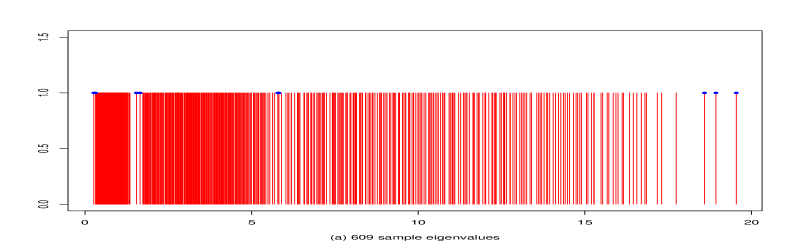
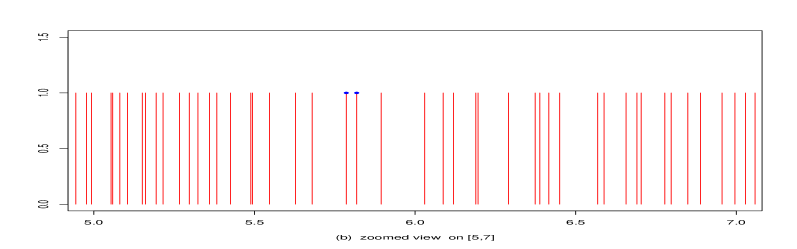
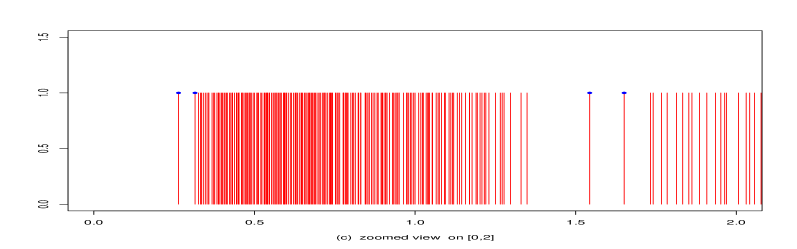
Figure 4. An example of $p=609$ sample eigenvalues (a), and two zoomed views (b) and (c) on [5,7] and [0,2] respectively. The limiting distribution of the E.S.D has support $[0.32,1.37]\cup[1.67,18.00]$. The 9 sample eigenvalues $\{\lambda_{j}^{S_{n}},\leavevmode\nobreak\ j=1,2,3,204,205,406,407,608,609\leavevmode\nobreak\ \}$ associated to the spikes are marked with a blue point. Gaussian entries.

There facts are illustrated by a simulation sample displayed in Figure 4.

5. CLT for sample eigenvalues from distant generalized spikes

Following Theorem 4.1, to any distant generalized spike eigenvalue $\alpha_{k}$, there is a packet of $n_{k}$ consecutive sample eigenvalues $\{\lambda_{j}^{S_{n}}:\leavevmode\nobreak\ j\in J_{k}\}$ converging to $\psi(\alpha_{k})\notin\Gamma_{G}$ where $J_{k}$ are the descending ranks of $\alpha_{k}$ among the eigenvalues of $T_{p}$ (counting multiplicities). The aim of this section is to derive a CLT for $n_{k}$-dimensional vector

$$\sqrt{n}\{\lambda_{j}^{S_{n}}-\psi(\alpha_{k})\}\leavevmode\nobreak\ ,\quad j\in J_{k}.$$

The method follows Bai and Yao [5] which considers Johnstone’s spiked population model. Consider the random form $K_{n}$ introduced in (2.2) and let

(5.1) $$A_{n}=(a_{ij})=A_{n}(\lambda)=X_{2}^{*}(\lambda I-X_{2}X_{2}^{*})^{-1}X_{2},\quad\lambda\notin\Gamma_{G}.$$

By Lemma 6.2, detailed in §6, we know that $n^{-1}trA_{n}$, $n^{-1}trA_{n}A_{n}^{*}$ and $n^{-1}\sum_{i=1}^{n}a_{ii}^{2}$ converge, almost surely or in probability, to $ym_{1}(\lambda)$, $ym_{2}(\lambda)$ and $\left({y[1+m_{1}(\lambda)]}/\{\lambda-y[1+m_{1}(\lambda)]\}\right)^{2}$, respectively. Here, the $m_{j}(\lambda)$ are some specific transforms of the LSD $G$ (see §6).

Therefore, the random form $K_{n}$ in (2.2) can be decomposed as follows

$$K_{n}(\lambda) = S_{11}+X_{1}A_{n}X_{1}^{*}=\frac{1}{n}\xi_{1:n}(I+A_{n})\xi_{1:n}^{*}$$

$$= \frac{1}{n}\left\{\xi_{1:n}(I+A_{n})\xi_{1:n}^{*}-\Sigma\mathrm{tr}(I+A_{n})\right\}+\frac{1}{n}\Sigma\mathrm{tr}(I+A_{n})$$

$$= \frac{1}{\sqrt{n}}R_{n}+\left[1+ym_{1}(\lambda)\right]\Sigma+o_{P}(\frac{1}{\sqrt{n}}),$$

with

(5.2) $$R_{n}=R_{n}(\lambda)=\frac{1}{\sqrt{n}}\left\{\xi_{1:n}(I+A_{n})\xi_{1:n}^{*}-\Sigma\mathrm{tr}(I+A_{n})\right\}.$$

In the last derivation, we have used the fact

$$\frac{1}{n}tr(I+A_{n})=1+ym_{1}(\lambda)+o_{P}(\frac{1}{\sqrt{n}}),$$

which follows from a CLT for $\mathrm{tr}(A_{n})$ [see 1].

For the statement of our result, we first need to find the limit distribution of the sequence of random matrices $\{R_{n}(\lambda)\}$. The situation is different for the real and complex cases. By applications of Propositions 3.1 and 3.2 in [5], we have for $\lambda\notin\Gamma_{G}$,

1. if the variables $(w_{ij})$ are real-valued, the random matrix $R_{n}(\lambda)$ converges weakly to a symmetric random matrix $R(\lambda)=(R_{ij}(\lambda))$ with zero-mean Gaussian entries having an explicitly known covariance function ;

2. if the variables $(w_{ij})$ are complex-valued, the random matrix $R_{n}$ converges weakly to a zero-mean Hermitian random matrix $R(\lambda)=(R_{ij}(\lambda))$. Moreover, the real and imaginary parts of its upper-triangular bloc $\{R_{ij}(\lambda),\leavevmode\nobreak\ 1\leq i\leq j\leq M\}$ form a $2K$-dimensional Gaussian vector with an explicitly known covariance matrix.

We are in order to introduce our CLT. Let the spectral decomposition of $\Sigma$,

(5.3) $$\Sigma=U\begin{pmatrix}\alpha_{1}I_{n_{1}}&\cdots&0\\ 0&\ddots&0\\ \cdots&0&\alpha_{K}I_{n_{K}}\end{pmatrix}U^{*}\leavevmode\nobreak\ ,$$

where $U$ is an unitary matrix. Let $\psi_{k}=\psi(\alpha_{k})$ and $R(\psi_{k})$ be the weak Gaussian limit of the sequence of matrices of random forms $[R_{n}(\psi_{k})]_{n}$ recalled above (in both real and complex variables case). Let

(5.4) $$\widetilde{R}(\psi_{k})=U^{*}R(\psi_{k})U\leavevmode\nobreak\ .$$

Theorem 5.3.

For each distant generalize spike eigenvalue, the $n_{k}$-dimensional real vector

$$\sqrt{n}\{\lambda_{j}^{S_{n}}-\psi_{k},\leavevmode\nobreak\ j\in J_{k}\}\leavevmode\nobreak\ ,$$

converges weakly to the distribution of the $n_{k}$ eigenvalues of the Gaussian random matrix

$$\frac{1}{1+ym_{3}(\psi_{k})\alpha_{k}}\widetilde{R}_{kk}(\psi_{k}).$$

where $\widetilde{R}_{kk}(\psi_{k})$ is the $k$-th diagonal block of $\widetilde{R}(\psi_{k})$ corresponding to the indexes $\{u,v\in J_{k}\}$.

It is worth noticing that the limiting distribution of such $n_{k}$ packed sample extreme eigenvalues are generally non Gaussian and asymptotically dependent. Indeed, the limiting distribution of a single sample extreme eigenvalue $\lambda_{j}^{S_{n}}$ is Gaussian if and only if the corresponding generalized spike eigenvalue is simple. We refer the reader to [5] for detailed examples illustrating these same facts but for Johnstone’s model.

6. Lemmas

For $\lambda\notin\Gamma_{G}$, we define

$$m_{1}(\lambda) = \int\frac{x}{\lambda-x}dG(x),$$

$$m_{2}(\lambda) = \int\frac{x^{2}}{(\lambda-x)^{2}}dG(x)\leavevmode\nobreak\ ,$$

$$m_{3}(\lambda) = \int\frac{x}{(\lambda-x)^{2}}dG(x)\leavevmode\nobreak\ .$$

The following lemma gives the law of large numbers for some useful statistics of $A_{n}$ defined in (5.1). We omit its proof because it is a straightforward extension of Lemma 6.1 of [5], related to Johnstone’s spiked population model, to the present generalized spiked population model.

Lemma 6.2.

Under the assumptions of Theorem 4.1, for all $\lambda\in[a,b]$, we have

(6.1) $$\frac{1}{n}trA_{n} \stackrel{{\scriptstyle a.s.}}{{\longrightarrow}} ym_{1}(\lambda)\leavevmode\nobreak\ ,$$

(6.2) $$\frac{1}{n}trA_{n}A_{n}^{*} \stackrel{{\scriptstyle a.s.}}{{\longrightarrow}} ym_{2}(\lambda)\leavevmode\nobreak\ ,$$

(6.3) $$\frac{1}{n}\sum\limits_{i=1}^{n}a_{ii}^{2} \stackrel{{\scriptstyle a.s.}}{{\longrightarrow}} \left(\frac{y[1+m_{1}(\lambda)]}{\lambda-y[1+m_{1}(\lambda)]}\right)^{2}.$$

Lemma 6.3.

For all $\lambda\in[a,b]$, $K_{n}(\lambda)$ converges almost surely to the constant matrix $[1+ym_{1}(\lambda)]\Sigma$.

Proof.

The random form $K_{n}$ in (2.2) can be decomposed as follows

$$K_{n}(\lambda)=S_{11}+X_{1}A_{n}X_{1}^{*}=\frac{1}{n}(\xi_{1},\ldots,\xi_{n})(I+A_{n})(\xi_{1},\ldots,\xi_{n})^{*}.$$

Define $M$ be the event that $S_{22}$ has no eigenvalues in the interval $[a^{\prime},b^{\prime}]$ which satisfies $[a,b]\subset(a^{\prime},b^{\prime})$ and $[a^{\prime},b^{\prime}]\subset(c,d)$. On the event $M$, the norm of $A_{n}$ is bounded by $\max\{\frac{1}{a-a^{\prime}},\frac{1}{b^{\prime}-b}\}$. By independence, it is easy to show that

$$\frac{1}{n}\left\{(u_{1},\ldots,u_{n})(I+A_{n})(u_{1},\ldots,u_{n})^{*}I_{M}-[\mathrm{tr}(I+A_{n})]I_{M}\right\}\stackrel{{\scriptstyle a.s.}}{{\to}}0.$$

By proposition 3.1, $I_{m}\to 1,a.s.$. Thus

(6.4) $$D_{n}(\lambda) = o_{a.s.}(1)++[\frac{1}{n}\mathrm{tr}(I+A_{n})]\Sigma I_{M}\stackrel{{\scriptstyle a.s.}}{{\to}}(1+ym_{1}(\lambda))\Sigma,$$

where the last step follows from (6.1). The conclusion follows. ∎

References

- Bai and Silverstein [2004] Z.D. Bai and J.W. Silverstein. CLT for linear spectral statistics of large-dimensional sample covariance matrices. Ann. Probab., 32:553–605, 2004.
- Bai and Silverstein [1998] Z.D. Bai and J.W. Silverstein. No eigenvalues outside the support of the limiting spectral distribution of large dimensional sample covariance matrices. Ann. Probab., 26:316–345, 1998.
- Bai and Silverstein [1999] Z.D. Bai and J.W. Silverstein. Exact separation of eigenvalues of large dimensional sample covariance matrices. Ann. Probab., 27(3):1536–1555, 1999.
- Bai and Silverstein [2006] Z.D. Bai and J.W. Silverstein. Spectral Analysis of Large Dimensional Random Matrices. Science Press, Beijing, 2006.
- Bai and Yao [2008] Z.D. Bai and J.-F. Yao. Central limit theorems for eigenvalues in a spiked population model. Ann. Inst. Henri Poincaré, 44(3):447–474, 2008.
- Baik and Silverstein [2006] J. Baik and J.W. Silverstein. Eigenvalues of large sample covariance matrices of spiked population models. J. Multivariate. Anal., 97:1382–1408, 2006.
- Baik et al. [2005] J. Baik, G. Ben Arous, and S. Péché. Phase transition of the largest eigenvalue for nonnull complex sample covariance matrices. Ann. Probab., 33(5):1643–1697, 2005.
- Capitaine et al. [2007] M. Capitaine, C. Donati-Martin, and D. Féral. The largest eigenvalue of finite rank deformation of large wigner matrices: convergence and non-universality of the fluctuations. Technical report, arXiv:math/0605624, 2007.
- Féral and Péché [2007] D. Féral and S. Péché. The largest eigenvalue of rank one deformation of large Wigner matrices. Comm. Math. Phys., 272(1):185–228, 2007.
- Johnstone [2001] I. Johnstone. On the distribution of the largest eigenvalue in principal components analysis. Ann. Statistics, 29(2):295–327, 2001.
- Marčenko and Pastur [1967] V.A. Marčenko and L.A. Pastur. Distribution of eigenvalues for some sets of random matrices. Math. USSR-Sb, 1:457–483, 1967.
- Péché [2006] S. Péché. The largest eigenvalue of small rank perturbations of Hermitian random matrices. Probab. Theory Related Fields, 134(1):127–173, 2006.
- Silverstein [1995] Jack W. Silverstein. Strong convergence of the empirical distribution of eigenvalues of large-dimensional random matrices. J. Multivariate Anal., 55(2):331–339, 1995.
- Silverstein and Choi [1995] Jack W. Silverstein and Sang-Il Choi. Analysis of the limiting spectral distribution of large-dimensional random matrices. J. Multivariate Anal., 54(2):295–309, 1995.