Making Sense of the Legendre Transform

Abstract

The Legendre transform is an important tool in theoretical physics, playing a critical role in classical mechanics, statistical mechanics, and thermodynamics. Yet, in typical undergraduate or graduate courses, the power of motivation and elegance of the method are often missing, unlike the treatments frequently enjoyed by Fourier transforms. We review and modify the presentation of Legendre transforms in a way that explicates the formal mathematics, resulting in manifestly symmetric equations, thereby clarifying the structure of the transform algebraically and geometrically. Then we bring in the physics to motivate the transform as a way of choosing independent variables that are more easily controlled. We demonstrate how the Legendre transform arises naturally from statistical mechanics and show how the use of dimensionless thermodynamic potentials leads to more natural and symmetric relations.

I Introduction

The Legendre transform is commonly used in upper division and graduate physics courses, especially in classical mechanics,CCC statistical mechanics, and thermodynamics.SM ; JWC Most physics majors are first exposed to the Legendre transform in classical mechanics, where it provides the connection between the Lagrangian $\mathcal{L}(\dot{q})$ and the Hamiltonian $\mathcal{H}(p)$, and then in statistical mechanics where it yields relations between the internal energy $E$ and the various thermodynamic potentials. Despite its common use, the Legendre transform often appears in an ad hoc fashion, without being presented as a general and powerful mathematical tool in the way the Fourier transform is.

In this paper we present a pedagogical introduction to the Legendre transform, discuss it as a mathematical process, and display some of its general properties. Since some students prefer algebraic approaches and some prefer geometric ones, we discuss the transform from both points of view and relate them. We then motivate the transform in terms related to physical conditions and constraints. We emphasize some of the symmetries and structures of the transform and present a series of increasingly complex examples beginning with classical mechanics and going through examples in statistical mechanics. We end with some remarks on more general versions of the Legendre transform, as well as other areas in which it is widely used.

II The Legendre transform as an alternative way to display information

In our experience, many students can manage the rules for generating a Hamiltonian from a Lagrangian or switching between thermodynamic potentials quite well, but express discomfort when asked about the Legendre transform as a general mathematical tool. One possible reason is that in introductory physics we often treat a function as a relation between physical rather than mathematical quantities. Thus, when we are thinking about physical functions we tend not to pay attention to the particular functional form the mathematical function uses to encode physical information.EFR For example, if we are describing a position as a function of time, we might write it as $x(t)$. We do not bother to change the symbol $x$ if we decide to give $t$ in milliseconds instead of in seconds. If we write the temperature as a function of position as $T(\vec{r})$, we do not change the symbol if we switch to a different coordinate system or measuring scale. In contrast, the Legendre transform is explicitly about how information is coded in the functional form.

In addition, students are usually first introduced to the Legendre transform as the transformation in classical mechanics from the Lagrangian to the Hamiltonian. This transformation involves the switch from the velocity to the momentum variable in the non-relativistic kinetic energy. In the context of non-relativistic particle motion with velocity independent potentials, the transform involves the kinetic energy, the most trivial function to which the Legendre transform can be applied. The result looks like a shift in units (from $v$ to $mv$ as an independent variable) so that it seems pointless. Because the position variable $q$ plays no role in the transform and typically appears only in $V$, the result is often regarded as a mysterious change of the sign of $V$: $\mathcal{L}=T-V$ vs. $\mathcal{H}=T+V$.

In the rest of this section we motivate the Legendre transform as a general mathematical transformation and describe a method that displays its general properties and symmetries.

For clarity, we begin with a single variable $x$ and consider multivariate functions later. Generally, a function expresses a relation between two parameters: an independent variable or control parameter $x$ and a dependent value $F$. This information is encoded in the functional form of $F(x)$. For later convenience, we will also denote such a relationship or “encoding” as $\left\{F,x\right\}$.

In some circumstances it is useful to encode the information contained in a function $F(x)$ in a different way. Two common examples are the Fourier transform and the Laplace transform. These transforms express the function $F$ as sums of (complex or real) exponentials, and display the information in $F$ in terms of the amount of each component contained in the function rather than in terms of the value of the function. In the notation introduced above, $\left\{\tilde{F},k\right\}$ encodes the same information as $\left\{F,x\right\}$. For the Fourier transform, $\tilde{F}\left(k\right)\equiv\int e^{ikx}F\left(x\right)dx$ is an explicit “transformation” between the two encodings.

Given an $F(x)$, the Legendre transform provides a more convenient way of encoding the information in the function when two conditions are met: (1) The function (or its negative) is strictly convex (second derivative always positive) and smooth (existence of “enough” continuous derivatives). (2) It is easier to measure, control, or think about the derivative of $F$ with respect to $x$ than it is to measure or think about $x$ itself.

Because of condition (1), the derivative of $F(x)$ with respect to $x$ can serve as a stand in for $x$; that is, there is a one-to-one mapping between $x$ and $dF/dx$. (We remark on relaxing this condition in the last section.) The Legendre transform shows how to create a function that contains the same information as $F(x)$ but as a function of $dF/dx$.

III The mathematics of the Legendre transform

We first consider a single, smooth convex function of a single variable. There are many equivalent ways to characterize convex functions. The most convenient one is that the second derivative $d^{2}F(x)/dx^{2}$ is always positive. A second characterization of our condition is that the slope function

$$s(x)\equiv\frac{dF(x)}{dx}$$ (1)

is a strictly monotonic function of $x$ (since this also permits us to treat functions whose negative is convex).

A graphical way to see how the value of $x$ and the slope of a convex function can stand in for each other can be seen by considering the example in Fig. 1, where the curve drawn to represent $F$ is convex. As we move along the curve to the right (as $x$ increases), the slope of the tangent to the curve continually increases. In other words, if we were to graph the slope as a function of $x$, it would be a smoothly increasing curve, such as the example in Fig. 2. If the second derivative $\frac{d^{2}F(x)}{dx^{2}}$ exists (everywhere within the range of $x$ in which $F$ is defined; part of the condition for a smooth $F$), there is a unique value of the slope for each value of $x$, and vice versa. The corresponding mathematical language is that there is a 1 to 1 relation between $s$ and $x$; that is, the function $s(x)$ is single-valued and can be inverted to give a single-valued function $x(s)$.

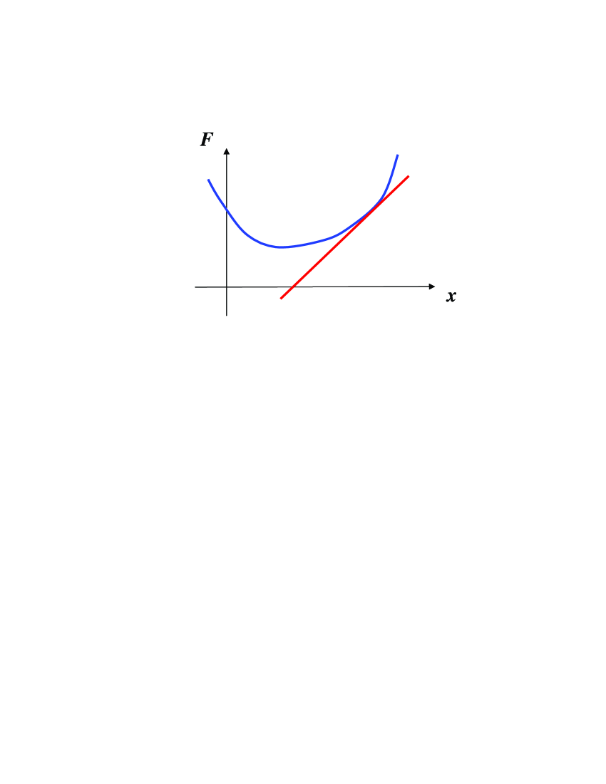
Figure 1: The graph (blue online) of a convex function$F\left(x\right)$. The tangent line at one point is illustrated (red online).

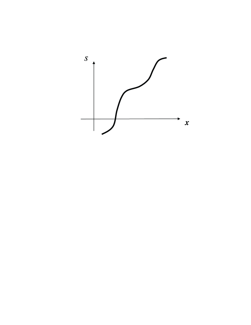
Figure 2: The graph of $s\left(x\right)$, the slope of a convex function.

In this way, we could then start with $s$ as the independent variable, use the inverse function to get an unique value of $x$, and then insert that into $F(x)$ to access $F$ as a function of $s$. The standard notation for such a function is $F(x(s))$. If we insist on a new encoding of the information in $F$ (in terms of $s$ instead of $x$), this straightforward “function of a function approach” would appear to be the most natural way.

Instead, the Legendre transform of $F(x)$ is defined quite differently, and seemingly quite unnatural:

$$G(s)=sx(s)-F(x(s))\,\,.$$ (2)

Typically, this formula is presented with little motivation or explanation, and leaves the students to ponder: Why? Why the extra $sx$? Why the minus sign? Frequently, the instructor or the author (of a textbook) invokes another magical relation to answer such queries. Only with this peculiar definition can we have the property that “the slope of $G(s)$ is just $x$”:

$$x(s)=\frac{dG}{ds}\,\,.$$ (3)

This result also requires a careful calculation.

III.1 A graphic-geometric approach

Before providing ways to appreciate this definition of the Legendre transform, as well as how never to forget “which sign goes where,” we present a graphical route to the transform. Consider the plot of $F$ versus $x$ in Fig. 3. Choose a value of $x$, which is represented by the length of the horizontal line labeled by $x$. Go up to the value on the function curve, $F(x)$. This value corresponds to the length of the vertical line labeled by $F$. Next, draw the tangent to the curve at that point. The slope here is labeled $s$, as emphasized by the call out bubble. Extend this tangent until it hits the ordinate (the “$F$ axis”). In this example, the intercept is negative and is labeled as $-G$, with a positive $G$. This value corresponds to the length of the thick vertical line labeled by $G$. This length is reproduced (thin line) just below the line labeled $F$. Because the slope of the tangent is $s$, the length of the dotted vertical line is $sx$. From this picture, it is quite clear that $sx=F+G$. In this light, the peculiar definition of the Legendre transform in Eq. (2) appears natural. The minus sign in the definition is seen as a way of retaining the symmetry and simplicity of the geometrical statement: “In the triangle, the slope (tangent) times the adjacent side equals the opposite side, which is the sum of $F$ and $G$.”

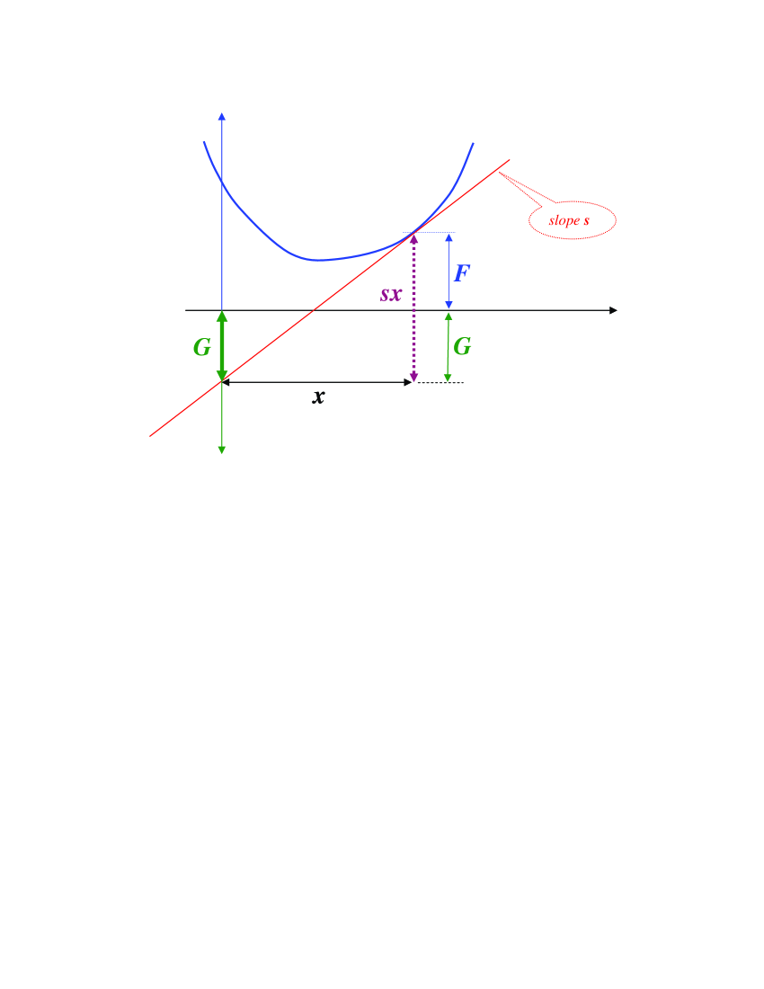
Figure 3: Graphic representation of the Legendre transform, $G\left(s\right)$, of $F\left(x\right)$. See text for an explanation of various quantities (color online).

III.2 Symmetric representation of the Legendre transform

This symmetric, geometrical construction allow us to display a number of useful and elegant relations that shed light on the workings of the Legendre transform. In particular, we consider the symmetries associated with the inverse Legendre transform, extreme values, and derivative relations.

Ordinarily, the inverse of a transformation is distinct from the transform itself. For example, an inverse Laplace transform is not given by the same formula. The Legendre transform distinguishes itself in that it is its own inverse. In this sense, it resembles (geometric) duality transformations. Symbolically, we may denote this relationship as:

$$\left\{F,x\right\}\Leftrightarrow\left\{G,s\right\}\,\,.$$ (4)

Specifically, if we perform the Legendre transform a second time, we recover the original function. (If the restriction of convexity is relaxed, this statement must be revised, as remarked in the final section.) In other words, suppose we start with the function $G(s)$ and calculate its Legendre transform. Of course, as we will see, $G(s)$ satisfies our conditions: convex and smooth. So, we start with

$$y(s)=\frac{dG}{ds}$$ (5)

and invert the monotonic function $y(s)$ to $s(y)$. Next, we construct

$$H(y)=ys(y)-G(s(y))\,\,,$$ (6)

which can be rewritten as

$$G=sy-H\,\,.$$ (7)

If we compare this equation and Eqs. (2), we see that we can identify $\{H,y\}$ with $\{F,x\}$. Thus, the Legendre transform of $G$ is the original function $F$, leading to the statement: the Legendre transform is its own inverse. This “duality” of the Legendre transform, shown symbolically in Eq. (4), is best displayed by the symmetric form

$$G(s)+F(x)=sx\,\,.$$ (8)

This equation should be read carefully. Despite its appearance, there is only one independent variable: either $s$ or $x$. Referred to as a conjugate pair, these two variables are related to each other, through either $x(s)=dG(s)/ds$ or $s(x)=dF(x)/dx$. A careful writing of Eq. (11) would read either $G(s)+F(x(s))=sx(s)$ or $G(s(x))+F(x)=s(x)x$. To double check the consistency with Eqs. (1) and (3), we can start with, say, the first of these equations and differentiate with respect to $s$. Applying the chain rule for $dF/ds=(dF/dx)(dx/ds)$, we recover $dG/ds=x$.

III.3 Properties of the extrema

The example in Fig. 3 shows a convex function $F(x)$ with a unique minimum. Let us denote this point by $F_{\min}=F(x_{\min})$. The slope of the tangent vanishes here, that is, $s(x_{\min})=0$. If we substitute this point into Eq. (2), we find that the minimum value of $F$ is

$$F_{\min}=-G(0)\,\,.$$ (9)

It is straightforward to show that a “dual” relation exists, namely, the minimum value of $G$ is $G_{\min}=-F(0).$ To appreciate the geometric meaning of this equation, we need only to inspect Fig. 3 and see that $-G$, the $y$-intercept of the tangent to the curve $F(x)$, never reaches beyond $F(0)$.

Exploiting Eq. (11), both this special example and the case of general extrema can be cast in an “easy-to-remember” symmetric form. Suppose $F$ takes on its extremal value at $x_{\mathrm{ext}}$, then we have a horizontal tangent line and by definition, $s(x_{\mathrm{ext}})=0$. Similarly, if $G$ is at its extremum at $s_{\mathrm{ext}}$, we have $x(s_{\mathrm{ext}})=0$ due to Eq. (3). In either case, the right hand side of Eq. (11) vanishes and we have

$$G(0)+F(x_{\mathrm{ext}})=0\quad\ \text{and}\ \quad G(s_{\mathrm{ext}})+F(0)=0\,\,.$$ (10)

III.4 Symmetric representation of the higher derivatives

Since the Legendre transform is a “dual” relationship, we can expect manifestly symmetric relations beyond the ones we have seen so far:

$$G(s)+F(x)=sx$$ (11)

and

$$\frac{dG}{ds}=x\quad\ \text{and}\ \quad\frac{dF}{dx}=s\,\,.$$ (12)

From these, we can obtain an infinite set of relations linking $G$ and $F$ by taking derivatives of $G+F=sx$ with respect to $s$ or $x$. Because each function depends on only one variable, the differentials can be easily identified. Thus, differentiating the equations in (12) with respect to $s$ or $x$ as appropriate, we find

$$\frac{d^{2}G}{ds^{2}}=\frac{dx}{ds}\quad\ \text{and}\ \quad\frac{d^{2}F}{dx^{2}}=\frac{ds}{dx}\,\,.$$ (13)

But $\left(dx/ds\right)(ds/dx)=1$, so we have

$$\left(\frac{d^{2}G}{ds^{2}}\right)\left(\frac{d^{2}F}{dx^{2}}\right)=1\,\,.$$ (14)

Let us emphasize once more that the variable $s$ in the first factor and the $x$ in the second are not independent, but linked through Eqs. (12)!

Equation (14) illustrates the importance of (strict) convexity so that neither derivative ever vanishes. An interesting result is that the local curvatures of the Legendre transforms are inverses of each other in a manner reminiscent of the uncertainty relation $\Delta x\Delta k\approx 1$. For simplicity, suppose $F$ is dimensionless but $x$ is not,note4 so that $s$ has the dimension of $1/x$. With this convention it is easy to check the units of Eqs. (11, 12, and 14).

If we differentiate Eq. (14) again, we can write a symmetric relation for the third derivative:

$$\frac{d^{3}G}{ds^{3}}\left[\frac{d^{2}G}{ds^{2}}\right]^{-3/2}+\frac{d^{3}F}{dx^{3}}\left[\frac{d^{2}F}{dx^{2}}\right]^{-3/2}=0\,\,.$$ (15)

Notice that each term is again dimensionless, since the units of the various derivatives precisely cancel.

It is possible to derive an infinite set of such relations for higher derivatives by differentiating further. Such an exercise also shows that if $F$ is smooth (with a well defined $n^{th}$ derivative), then so is $G$. The relations for higher derivatives do not have forms as simple as Eqs. (11), (12), (14) and (15), but become more and more complex.

IV Examples of the Legendre transform in single-particle mechanics

It is useful to provide some physical examples to illustrate these relations. The simplest is a quadratic function $F(x)=\alpha x^{2}/2$. For this function we easily find that $s=\alpha x$ and $x=s/\alpha$, leading to $G(s)=s^{2}/2\alpha$. The curvatures in $F$ and $G$ ($\alpha$ and $1/\alpha$, respectively) are inverses of each other as required by Eq. (14). All derivative relations beyond this level are trivial, i.e., $0=0$.

This example corresponds to a single non-relativistic particle with mass $m$ moving in an external potential $V(q)$. The Legendre transform connects the Lagrangian $\mathcal{L}(\dot{q})$ to the Hamiltonian $\mathcal{H}(p)$. Only the kinetic term, which depends on $\dot{q}$ or $p$ is affected by the transform, as the potential depends on an entirely different variable: $q$. There, $x\to\dot{q}$, $F\to\mathcal{L}$, $\alpha\to m$, $s\to p$, and $G\to\mathcal{H}$, so that $\mathcal{L}=m\dot{q}^{2}/2\Leftrightarrow\mathcal{H}=p^{2}/2m$. However, since $V(q)$ is just a “spectator” in the Legendre transform, it must appear with opposite signs in $F$ and $G$ (i.e., $\mathcal{L}$ and $\mathcal{H}$), in order to satisfy $F+G=sx$ (i.e., $\mathcal{L}+\mathcal{H}=p\dot{q}$, with no $q$ anywhere). Thus, we see the origin of the mysterious sign change in $V$ when we go from the Hamiltonian to the Lagrangian.

Relativistic kinetic energy is a more interesting case. Here, we go the other way and start with momentum and generate a velocity as the slope of the function. The relativistic kinetic energy as a function of momentum is $\mathcal{H}(p)=\sqrt{p^{2}+m^{2}}$ (with $c\equiv 1$). $\mathcal{H}(p)$ is convex and its slope at a point $p$ is

$$v\equiv\frac{d\mathcal{H}}{dp}=\frac{p}{\sqrt{p^{2}+m^{2}}}\,\,,$$ (16)

giving the familiar result

$$p=mv/\sqrt{1-v^{2}}\,\,.$$ (17)

Creating the Legendre transform using this pair of variables leads to the LagrangianJDJ

$$\mathcal{L}(v)=pv-\mathcal{H}(p(v))=-m\sqrt{1-v^{2}}\,\,.$$ (18)

This example can also be written in terms of the function $F(x)=\cosh\lambda x$. The demonstration is left to the reader. (Hint: see Ref. TW, .)

Let us turn to a less familiar example, one that is so trivial that it does not appear in typical textbooks. Yet it sets the stage for examining the role of the Legendre transform in equilibrium statistical mechanics.

Consider a particle in a one-dimensional convex potential well, $U(x)$, which has a unique minimum at $x_{\min}$. An example would be a particle attached to a wall by a non-ideal spring, with $x$ being the distance from the point where the coils of the spring are fully compressed. The potential is effectively infinite at $x=0$, decreases to a minimum at its natural extension, and then increases for larger $x$. (We restrict our attention to positive values of $x$, but less than the breaking point of the spring.) Another example of $U$ is the potential that binds two atoms into a molecule (though such $U$’s are rarely convex for all separations).

The particle is stationary only if it is at $x_{\min}$ for all time. If it is subjected to an additional external applied force $f$, then it will reach a new stationary point $x_{0}$, which is the solution to the equation

$$\left.\frac{dU}{dx}\right|_{x_{0}}=f\,\,.$$ (19)

To emphasize the dependence of this point on $f$, we write $x_{0}(f)$. We can ask the inverse question: If we want the particle to settle at $x_{1}\neq x_{\min}$, what force do we need to apply? The answer is $f(x_{1})$, a force that depends on which $x$ we choose. A little thought leads us to the explicit functional form: $f(x_{1})=dU/dx|_{x_{1}}$. There is nothing special about the subscripts here and we may just as well write

$$f(x)=\frac{dU}{dx}\,\,,$$ (20)

and $x(f)$ instead of $x_{0}(f)$.

Although Eq. (20) gives $f(x)$ explicitly, we may ask if there is a counterpart to $U$ which provides the inverse, $x(f)$, explicitly. If so, we can simply plug $f$ into the expression and arrive at the new equilibrium position. The answer is the Legendre transform of $U$, namely, $V(f)=fx-U(x(f))$. We leave it to the reader to show that

$$x(f)=\frac{dV}{df}$$ (21)

is the companion to Eq. (20).

All the details can be worked out for the simple example of the mass on a spring, $U(x)=kx^{2}/2$. This example is the analog of the non-relativistic kinetic energy Legendre transform. The reader can easily demonstrate that the Legendre transform equation $U+V=fx$ becomes $(f-kx)^{2}=0$, yielding the relation between $f$ and the new equilibrium point $x$.

Note that the information about the system (for example, wall-spring-particle complex) is fully contained in either $U$ or $V$. The only difference is in the coding: $\left\{U,x\right\}$ vs. $\left\{V,f\right\}$. Although $U$ is the usual potential energy associated with putting the particle at $x$, $V$ is a kind of potential associated with the control $f$. In ordinary classical mechanics, such an approach seems unnecessarily cumbersome for describing the simple problems we posed. Thus, it is rightfully ignored in a course on classical mechanics. We include the example here only as a stepping stone to the Legendre transform in statistical mechanics and thermodynamics. There, multiple potentials are essential.

V The Legendre transform in statistical thermodynamics

The Legendre transform appears frequently in statistical thermodynamics when different variables are “traded” for their conjugates. SM Often, one of the variables is easy to think about while the other is easy to control in physical situations.

The difficulty with making sense of the Legendre transform in thermodynamics arises from two causes: (1) For historical reasons, Legendre transform variables are not always chosen as conjugate pairs. (2) Many variables in thermodynamics are not independent and are constrained by equations of state, for example, $PV=Nk_{B}T$.

As an example of the first point, the conjugate to the total energy $E$ of a system is the inverse temperature ($\beta=1/k_{B}T$). Yet, our daily experience with the temperature $T$ is so pervasive that $T$ is used in most of the relations. Thus, the familiar equation

$$F=E-TS\,\,,$$ (22)

which relates the Helmholtz free energy $F$ to the entropy $S$, obscures the symmetry between $\beta$ and $E$, as well as the dimensionless nature of the Legendre transform. In contrast, if we define the dimensionless quantities

$$\mathcal{S}\equiv S/k_{B}\ \text{and}\ \mathcal{F}\equiv\beta F\,\,,$$ (23)

the “duality” between them can be beautifully expressed as

$$\mathcal{F}(\beta)+\mathcal{S}(E)=\beta E\,\,.$$ (24)

To elaborate the second point, we typically encounter a bewildering array of thermodynamic functions (for example, entropy, Gibbs and Helmholtz free energies, and enthalpy), a slew of variables (energy, temperature, volume, and pressure), as well as a jumble of thermodynamic relations (with multiple partial derivatives). In general, because of the multiple constrained variables, none of these examples is as simple as those we have considered, compounding the difficulty of both teaching and learning this material.

Before discussing the generation of the standard thermodynamic potentials, we briefly summarize the basics of statistical mechanics. We will show how the Legendre transform enters thermodynamics through the Laplace transform of partition functions in statistical mechanics.

Equilibrium statistical mechanics is based on the hypothesisSM that for an isolated system, every allowed microstate is equally probable. The high probability of finding a particular equilibrium macrostate is due to a predominance of the number of microstates corresponding to that macrostate. The classic example is a gas of $N$ identical, free, non-relativistic structureless particles, confined in a $D$-dimensional box of volume $L^{D}$. For this system a microstate is specified by the $2DN$ variables corresponding to the positions and momenta of each particle, $\{\vec{r}_{i},\vec{p}_{i}\}$, with $i=1,\ldots,N$. Because the total energy $E$ is a constant for an isolated system, the fundamental hypothesis can be represented as

$$P\left(\{\vec{r}_{i},\vec{p}_{i}\}\right)\propto\delta\left(E-\mathcal{H}(\{\vec{r}_{i},\vec{p}_{i}\})\right)\,\,,$$ (25)

where $P\left(\{\vec{r}_{i},\vec{p}_{i}\}\right)$ is the probability of finding the configuration of positions and momenta $\{\vec{r}_{i},\vec{p}_{i}\}$ and $\mathcal{H}$ is the Hamiltonian. In this case $\mathcal{H}$ is explicitly given by

$$\mathcal{H}=\sum_{i}h(\vec{r}_{i},\vec{p}_{i})=\sum_{i}\left[\frac{\vec{p}_{i}^{2}}{2m}+U(\vec{r}_{i})\right]\,\,,$$ (26)

where $m$ is the mass of each particle and $U$ is the confining potential, which is zero for each component of $\vec{r}\in[0,L]$ and infinite otherwise.

The normalization factor for $P$ is

$$\Omega(E)=\!\int_{r,p}\!\delta\left(E-\mathcal{H}(\{\vec{r}_{i},\vec{p}_{i}\})\right)\,\,,$$ (27)

where the integral is over all $\{\vec{r}_{i},\vec{p}_{i}\}$ from $-\infty$ to $\infty$. (The infinite values of $U$ restrict the actual position integrations to the volume of the box.) We have also suppressed the other variables that $\Omega$ depends on for now: $L$ and $m$. Note that $\Omega$ is just the volume of phase space available for our system and is also known as the microcanonical partition function.

The standard approach evaluates the integral in Eq. (27) as follows. The position integrals can be done explicitly because the only dependence of the Hamiltonian on position is the confinement of the position integrals to the allowed volume. These integrals yield a factor of $L^{ND}$. The momentum integrals are done by computing the surface area of a sphere in $DN$ dimensions.

The entropy is introduced by the definition $S\equiv k_{B}\ln\Omega$. We exploit the “dimensionless entropy” $\mathcal{S}$ and write

$$\mathcal{S}(E)\equiv\ln\Omega(E)\,\,.$$ (28)

To proceed, we have two choices: the route that emphasizes the mathematics or the physics.

V.1 The route of mathematics

Our task is straightforward: evaluate integrals with a constraint such as Eq. (27). Often, such integrals are not easy to perform. However, exploiting the Laplace transform typically renders the integrand factorizable. For example, the $DN$ integrations in Eq. (27) become products of a single integral. Specifically, we consider the Laplace transform of $\Omega(E)$,

$$Z(\beta)\equiv\!\int\!\Omega(E)e^{-\beta E}dE\,\,.$$ (29)

If we substitute Eq. (27) for $\Omega(E)$, the delta function permits us to do the $E$ integral giving

$$Z(\beta)=\!\int_{r,p}\!e^{-\beta\mathcal{H}}\,\,.$$ (30)

Because $\mathcal{H}$ is a sum over the individual components, the integrand factorizes and we have the result:

$$\int_{r,p}e^{-\beta\mathcal{H}}=\!\int_{r,p}\prod_{i}e^{-\beta h(\vec{r}_{i},\vec{p}_{i})}=\left[\int d\vec{r}d\vec{p}e^{-\beta h(\vec{r},\vec{p})}\right]^{N}.$$ (31)

Being an integral in just $2D$ dimensions, the expression in $\left[...\right]$ is much easier to handle. For the classic example above, the integral is simply $L^{D}\left(2\pi m/\beta\right)^{D/2}$. The attentive student will have noticed, from Eq. (30) that $Z$ is the canonical partition function and can appreciate the statement: The two partition functions are related to each other through a Laplace transform.

To return to our goal, $\Omega(E)$, we need to perform an inverse Laplace transform, that is,

$$\Omega(E)=\!\int_{\mathcal{C}}\!Z(\beta)e^{\beta E}d\beta\,\,,$$ (32)

where $\mathcal{C}$ is a contour in the complex $\beta$ plane (running parallel to and to the right of the imaginary axis). We define

$$\mathcal{F}(\beta)\equiv-\ln Z(\beta)\,\,,$$ (33)

and write the integral as

$$e^{\mathcal{S}(E)}=\!\int_{\mathcal{C}}e^{-\mathcal{F}(\beta)+\beta E}d\beta\,\,.$$ (34)

To continue it is necessary to inject some physics. In this case, we expect to be considering many particles, that is, large $N$. From Eq. (31), we have $\mathcal{F}\propto N$, leading us to expect that the range of $E$ of interest is also $O(N)$. The standard tool to evaluate integrals with large exponentials as integrands is the saddle point (or steepest decent) method. Thus, we seek the saddle point in $\beta$, defined by setting the first derivative of $\beta E-\mathcal{F}(\beta)$ to zero:

$$\left.\frac{d[\beta E-\mathcal{F}]}{d\beta}\right|_{\beta_{0}}=0\,\,.$$ (35)

In other words, we have

$$\left.\frac{d\mathcal{F}}{d\beta}\right|_{\beta_{0}}=E\,\,.$$ (36)

We emphasize that $\beta_{0}$ should be regarded as a function of $E$ here.

In this approach, the integral in Eq. (29) is well approximated by evaluating the integrand at the saddle point, so that

$$\Omega(E)\cong\exp[\beta_{0}E-\mathcal{F}(\beta_{0})]\,\,,$$ (37)

or using Eq. (28)

$$\mathcal{S}(E)+\mathcal{F}(\beta_{0})=\beta_{0}E\,\,,$$ (38)

with the understanding that $\beta_{0}$ and $E$ are related through Eq. (36). There is nothing significant about the subscript on $\beta$ and Eq. (38) is identical to Eq. (24). In other words, $\mathcal{S}$ and $\mathcal{F}$ are Legendre transforms of each other. Thus, we see that (for situations involving a large parameter, $N$ in this case) the Laplace and Legendre transforms, Eqs. (29) and (38) respectively, are intimately related to each other as a result of the thermodynamic limit.

V.2 The route of physics: interpretation of the equilibrium condition

Under what conditions does the internal energy move from one object to another and under what conditions can it be changed to work? Part of the answer lies in understanding which way the energy will move if we bring two different systems into thermal contact. Why does it not go always from the system with more energy to the one with less? Considering this question leads us back to the Legendre transform.

When two systems (not necessarily of the same size or energy) are brought together and the combined system isolated, $E_{\mathrm{tot}}\equiv E_{1}+E_{2}$ will remain a constant and can be regarded as the control parameter. The individual $E_{j}$’s are not fixed, and we ask the question: Starting at some initial values, how do they wind up at the final equilibrium partition $\{E_{1}^{*},E_{2}^{*}\}$? The answer lies with $\mathcal{S}_{\mathrm{tot}}(E_{\mathrm{tot}}|E_{1},E_{2})$, the entropy of the combined system subjected to the specific partition of $E_{\mathrm{tot}}$ into $\{E_{1},E_{2}\}$. The idea is $e^{\mathcal{S}_{\mathrm{tot}}}$ counts the number of allowed microstates associated with a particular partition and so, carries the information of how probable that partition is. In general, calculating this quantity is not trivial. However, if we focus on systems with extensive entropies, then we may write to a good approximation: $\mathcal{S}_{\mathrm{tot}}=\mathcal{S}_{1}+\mathcal{S}_{2}$ with $\mathcal{S}_{1}=\mathcal{S}_{1}(E_{1})$ and $\mathcal{S}_{2}=\mathcal{S}_{2}(E_{2})$. These statements are not trivial: We are injecting the physics that, under the conditions specified, the entropies of each system do not depend on the energy of the other.

Given these assumptions we can ask for what partition will $\mathcal{S}_{\mathrm{tot}}$ be maximum, or equivalently, which partition is the most probable? If we write $E_{2}=E_{\mathrm{tot}}-E_{1}$ and recall that $E_{\mathrm{tot}}$ is fixed, this task is easy. The maximum occurs at $E_{1}^{*}$, defined by

$$\frac{d\mathcal{S}_{\mathrm{tot}}}{dE_{1}}|_{E_{1}^{*}}=0\,\,.$$ (39)

But $dE_{1}=-dE_{2}$, so that we have

$$\frac{d\mathcal{S}_{1}}{dE_{1}}|_{E_{1}^{*}}=\frac{d\mathcal{S}_{2}}{dE_{2}}|_{E_{2}^{*}}\,\,,$$ (40)

where $E_{2}^{*}=E_{\mathrm{tot}}-E_{1}^{*}$. This result is significant because each side does not depend on the parameters of the other system. Thus, if we associate a quantity with $d\mathcal{S}/dE$, which we define by

$$\beta(E)\equiv\frac{d\mathcal{S}}{dE}\,\,,$$ (41)

then Eq. (40) becomes

$$\beta_{1}(E_{1}^{*})=\beta_{2}(E_{2}^{*})\,\,.$$ (42)

In other words, the most probable partition occurs when the $\beta$ of one system equals the $\beta$ of the other. Note that this condition does not depend on the details of the two systems, such as composition, size, or state (gas, liquid, solid, etc.). When the two systems are brought into contact, energy will flow between them until they settle at values given by this condition: the equality of a quantity, $\beta\equiv d\mathcal{S}/dE$, associated with each of them separately. It is natural, therefore, to use this quantity for describing our daily experience, namely, two systems, one hot and one cold, will equilibrate at a common “temperature” ($T$) when brought in contact with each other. Historically, many arbitrary scales were used for $T$. Their relationships with the more natural quantity $\beta$ were not clarified later.

Besides providing a natural scale to describe “hot” and “cold,” can this variable $\beta$ be exploited further? For a given system, we can write $\mathcal{S}(E(\beta))$, but is that useful? The answer is connected to the canonical ensemble, the (Helmholtz) free energy, and the Legendre transform of $\mathcal{S}$. There is no need to reproduce here the standard derivation of this ensemble and the Boltzmann factor $e^{-\beta\mathcal{H}}$. In the previous subsection, we have already discussed the transformation between the partition functions $Z(\beta)$ and $\Omega(E)$ and the relationship to the Legendre transform between $\mathcal{S}(E)$ and $\mathcal{F}(\beta)$.

V.3 How does the Legendre transform enter into thermodynamics?

For convenience we summarize the key relations using dimensionless potentials:

$$\Omega(E)=e^{\mathcal{S}(E)}\,\,,\,\, Z(\beta)=e^{-\mathcal{F}(\beta)}\,\,,$$ (43)

$$\frac{d\mathcal{S}}{dE}=\beta\,\,,\,\, \frac{d\mathcal{F}}{d\beta}=E\,\,,$$ (44)

where $Z\left(\beta\right)=\int dEe^{-\beta E}\Omega(E)$ and, in the thermodynamic limit, $\mathcal{F}(\beta)+\mathcal{S}(E)=\beta E$. We can now see where the Legendre transform enters and why it is useful. The entropy $\mathcal{S}$ is a function of $E$, but the internal energy is typically not easy to control. To put more energy into a system (or take some out), we may give it some heat (or remove some). In other words, we often manipulate $E$ by coupling the system to an appropriate thermal bath and so, temperature (or $\beta$) becomes the “control” variable. In that case, we can perform a Legendre transform of $\mathcal{S}\left(E\right)$ and work with $\mathcal{F}(\beta)$ instead. Since both $\left\{\mathcal{S},E\right\}$ and $\left\{\mathcal{F},\beta\right\}$ contain the same information about our system, it makes sense to deal with the more convenient thermodynamic potential when we change the control on our system from one variable to another.

Since the independent variable in a thermodynamic potential is to be regarded as a control (or a constraint) parameter, the “slope” associated with this function (e.g., $d\mathcal{S}/dE$, $d\mathcal{F}/d\beta$) carries physically significant information, namely, the response of the system to this control. The Legendre transform simply exchanges the role of the variables associated with control and response. For the example discussed above, it is physically easier to control $T$. It is also more familiar to think of temperature (or $\beta$) as a control and the internal energy as the response. Thus, the free energy $\mathcal{F}(\beta)$ is the more appropriate potential, with $E=d\mathcal{F}/d\beta$ being the response. In the transformed version, which is mathematically and conceptually easier to grasp, $E$ is a constraint (conserved variable for an isolated system) and $\mathcal{S}\left(E\right)$ is the more appropriate potential. After we understand the significance of its slope, $d\mathcal{S}/dE$, we can identify the “response” $\beta$ with a measure for temperature. There are many other examples of response/control pairs to which the same kind of transformation may be applied, such as particle number and chemical potential, polarizability and electric field, magnetization and magnetic field, etc.

VI Legendre transform with many variables

The thermodynamic potentials depend on many variables other than just the total energy $E$. Each variable that can be independently controlled elicits a distinct response. As we construct Legendre transforms for each of these control/response variable pairs, we generate a new potential. The result is a plethora of thermodynamic functions. We again emphasize that all these thermodynamic potentials carry the same information, but encoded in different ways. We begin this section by discussing briefly the mathematical structure of the multivariable Legendre transform and then apply it to thermodynamics and statistical mechanics.

Consider the multivariate function $F(\vec{x})$, where $\vec{x}$ stands for $M$ independent variables: $x_{1},\ldots,x_{M}$. For convenience, suppose $F$ is smooth and convex over all of this $M$-dimensional space. At every point $\vec{x}$, there will be $M$ slopes:

$$s_{m}=\frac{\partial F}{\partial x_{m}}\equiv\partial_{m}F\,\,,$$ (45)

and $M(M+1)/2$ second derivatives, $\partial_{m}\partial_{\ell}F$, which can be regarded as a symmetric matrix. The convexity restriction requires that all of the eigenvalues of this matrix are positive (or negative).CUR In the context of thermodynamics, convexity is the condition for stability in equilibrium systems.note7 A standard corollary is that the relation between $\{x_{m}\}$ and $\{s_{m}\}$ is 1 to 1, so that we can replace any one of the $x_{m}$’s by the corresponding $s_{m}$ through a Legendre transform.

Because we can transform any number of the $x$’s, we may consider (up to) $2^{M}$ functions. For example, if we restrict ourselves to $(E,V)$ – the standard variables for the microcanonical ensemble of the ideal gas – there are four thermodynamic functions: entropy, enthalpy, Gibbs, and the Helmholtz free energies. One way to picture the relation between so many functions is to put them at the corners of an $M$-dimensional hypercube. Each axis in this space is associated with a particular variable pair $(x_{m},s_{m})$. Going from one corner to an adjacent corner along a particular edge corresponds to carrying out the Legendre transform for that pair. For the $M=2$ example of $(x_{1},x_{2})=(E,V)$, the hypercube reduces to a square, which is related, but not identical, to the square that appears in some texts.SM ; note8 Thanks to the commutativity of partial derivatives, going from any corner to any other corner is a path independent process, so that the function associated with each vertex is unique. For example, if we exchange $(x_{\ell},x_{m})$ for $(s_{\ell},s_{m})$, the Legendre transform relations would be the simple generalization of Eq. (11)

$$F(x_{1},\ldots x_{\ell},\ldots x_{m},\ldots x_{M})+G(x_{1},\ldots s_{\ell},\ldots s_{m},\ldots x_{M})\\ =s_{\ell}x_{\ell}+s_{m}x_{m}\,\,,$$ (46)

withnote9 $\partial_{\ell}G=x_{\ell}$, $\partial_{m}G=x_{m}$, $\partial_{\ell}F=s_{\ell}$, and $\partial_{m}F=s_{m}$. We should have given this $G$ some special notation to denote that its variables are all $\{x\}$ except for the two that are $\{s\}$. A possibility is $G^{\ell,m}$, but for simplicity, we do not pursue this issue further. One special Legendre transform is noteworthy – the one in which all variables are $\{s\}$. Located at the corner of the hypercube diametrically opposite to $F$, this function will be denoted by $H$. In this case, the Legendre transform relation simplifies to

$$H(\vec{s})+F(\vec{x})=\vec{s}\cdot\vec{x}\,\,.$$ (47)

Generalizations for higher derivatives proceed are straightforward. For example, Eq. (14) becomes

$$\sum_{m}(\partial_{\ell}\partial_{m}H)(\partial_{m}\partial_{n}F)=\delta_{\ell n}\,\,,$$ (48)

where $\delta$ is the unit matrix. The convexity of $F$ guarantees that the inverse of $\partial_{m}\partial_{n}F$ exists.

Let us apply these considerations to the thermodynamics of a gas. We begin with the microcanonical partition function $\Omega(E,V)$ and consider the mapping

$$F(x_{1},x_{2})\to\mathcal{S}(E,V)\equiv\ln\Omega\,\,,$$ (49)

$x_{1}\rightarrow E$, $x_{2}\rightarrow V$, $s_{1}\rightarrow\beta$, $s_{2}\rightarrow\eta$. The last of these is related to the pressure $P$, an issue we will comment on later. The Legendre transform with respect to $x_{1}$ leads to the Helmholtz free energy. Our symmetric and dimensionless version of $F=E-TS$ is same as Eq. (24): $\mathcal{F}(\beta,V)+\mathcal{S}(E,V)=\beta E$, with $V$ playing the role of a “spectator.” Thus, to be precise, we now write Eq. (41) with a partial derivative:

$$\beta\equiv\left.\frac{\partial\mathcal{S}}{\partial E}\right|_{V}\,\,.$$ (50)

For the second Legendre transform, with respect to $x_{2}=V$, we define note10

$$\eta\equiv\left.\frac{\partial\mathcal{S}}{\partial V}\right|_{E}$$ (51)

and arrive at

$$\mathcal{G}(\beta,\eta)+\mathcal{S}(E,V)=\beta E+\eta V\,\,.$$ (52)

Here, $\mathcal{G}\equiv\beta G(T,P)$ is the dimensionless Gibbs free energy. Meanwhile, the relationship between $\eta$ and the traditional definition of pressure, $P\equiv\left.-\partial E/\partial V\right|_{S}$, is $\eta=\beta P$. To show this will take us further afield, into the first law of thermodynamics and the notion of heat transfer. The interested reader may consult a standard text, such as Ref. note10, .

Returning to Eq. (52), we move $\mathcal{S}$ and divide both sides by $\beta$ to arrive at its more common form: $G=E-TS+PV$. The seemingly mysterious signs of the last two terms on the right are, from our perspective, due to the placing of $S$ and the use of $T$ instead of $\beta$. By contrast, every term comes with a positive sign in Eq. (52), with all the potentials on the left and all the conjugate variables on the right. Note that there are just two variables in this example, so that $\mathcal{G}$ plays the role of $H$ in Eq. (47), which is an explicit writing of Eq. (52) here.

Lastly, we turn to enthalpy, which is laden with extra complications. For various reasons, $S$ (instead of $E$) is chosen to be the independent variable for arriving at the enthalpy. As a result, instead of $\beta$, the natural conjugate variable is $T$ ($=\partial E/\partial S$). Regarding $S$ as a control variable with which to access $E$ is conceptually difficult. However, it is common to think of transferring heat so that $TdS$ appears as the means of control. If we take the Legendre transform of $E(S)$ in the standard fashion, we would arrive at $TS-E$, which is the Helmholtz free energy except for a sign. The disadvantage is clear, but there are advantages to this approach. In particular, by starting with $E(S,V)$, we naturally arrive at the ordinary pressure, $-P$, as the conjugate to $V$ (instead of $\eta$). Note the extra minus sign here. The Legendre transform with respect to $V$ of $E(S,V)$ gives $(-P)V-E$, the (negative of) enthalpy $H=E+PV$. If we allow logic to overcome tradition, we would have defined the last potential as $\mathcal{H}(E,\eta)$ (not to be confused with the Hamiltonian $\mathcal{H}$!) through the Legendre transform

$$\mathcal{H}(E,\eta)+\mathcal{S}(E,V)=\eta V\,\,,$$ (53)

in which the first variable, $E$, plays the role of a spectator. But, the beauty of pure reason does not always prevail and we must often abide by the results of our historical paths.

VII Concluding remarks

There are many interesting aspects of the Legendre transform we have not discussed. Covering all aspects would be more appropriate for a textbook than a journal article. Here, let us conclude by touching on just two important generalizations - the Legendre transform of (a) non-convex functions and (b) functions defined on spaces with non-trivial topology, such as the angle on a circle - and providing references for further reading.

If a function is non-convex, the Legendre transform becomes multi-valued. If we delete all but the principal branch, the Legendre transform develops discontinuous first derivatives. If we perform another transformation, the result would be the convex hull of the original. This topic is intimately related to the Maxwell construction and the co-existence of phases (for example, liquid and vapor). Although most texts on thermodynamics and statistical mechanics discuss the Maxwell construction, few demonstrate its relation to the Legendre transform of non-convex functions. The interested reader may find a good example of a convexified (free energy) function in Ref. Schroeder, .

A second generalization concerns variables whose domains have a non-trivial topology, the simplest being functions defined on a circle or the surface of a sphere. The angles are the most natural variables for a sphere, but we must be mindful of the periodic nature of $\phi\in(0,2\pi]$ and the co-ordinate singularities at the poles $\theta=0,\pi$. An example is the shape of crystals in equilibrium with its liquid (for example, ⁴He crystals in coexistence with the superfluid He4 ) or vapor (for example, gold crystalsAu ). Typical crystal shapes are not spherical and can be described by a non-trivial function $R(\theta,\phi)$, which specifies the distance from the center of mass to a point on the crystal surface labeled by $(\theta,\phi)$. The tangent plane at that point can be associated by the direction of its normal and labeled by $(\tilde{\theta},\tilde{\phi})$. The relation between these and the derivatives $\partial_{\theta}R$ and $\partial_{\phi}R$ exists, but is not simple. From these derivatives a (generalized) Legendre transform of $R$ can be constructed: $\sigma(\tilde{\theta},\tilde{\phi})$. The function $\sigma$ is also a significant physical quantity: it is the free energy per unit area (surface tension) associated with a planar interface, with normal $(\tilde{\theta},\tilde{\phi})$, between the crystalline and the isotropic phases of the material. A bonus is that, unlike typical thermodynamic potentials such as the entropy and free energies, the “potential” $R(\theta,\phi)$ is not just an abstract concept; it can be visualized, being displayed explicitly as a shape in three dimensions. Further details of this intriguing connection may be found in Refs. ECS, .

Finally, we should point the readers to horizons far beyond those discussed here. Since our purpose is to reach students and instructors in upper undergraduate and core graduate courses, we limit our considerations to cases with two (or finite $M$) variables above. Beyond this level, it is possible to study the Legendre transform with an infinite number of variables. Probably the most well known example in physics comes from both quantum field theoryQFT and statistical field theorySFT . Associated with each quantum field $\phi\left(\vec{r},t\right)$ is a “source field” $J\left(\vec{r},t\right)$, in much the same way that a fluctuating local magnetization, $m\left(\vec{r}\right)$, can be “created” by an inhomogeneous magnetic field $B\left(\vec{r}\right)$. In the latter system, the fluctuations of $m$ are thermal, rather than quantum, in nature. Now, the source field can be regarded as a control variable for each $\vec{r},t$ (or just $\vec{r}$). Thus, there are an infinite number of variables, as well as responses, involved. Corresponding to a given $J\left(\vec{r},t\right)$ or $B\left(\vec{r}\right)$, we can compute, in principle, the “vacuum energy” $\mathcal{U}\left[J\left(\vec{r},t\right)\right]$ or the free energy $\mathcal{F}\left[B\left(\vec{r}\right)\right]$. These carry information on the quantities of interest: connected Schwinger functions (expectation values of products of $\phi$’s) or correlations functions (averages of products of $m$’s). More useful than $\mathcal{U}$ is its Legendre transform, $\Gamma$. Known as the effective action, $\Gamma$ displays the essential information more conveniently in terms of one particle irreducible (1PI) Schwinger functions or vertex functions. For the effective action of a quantum field, there is a particularly appealing systematic expansion: in powers of $\hbar$. The zeroth order term is just the classical action. Similarly, for the Legendre transform of $\mathcal{F}$, there is a systematic expansion in powers of $T$ or $\beta^{-1}$. Not surprisingly, the zeroth order term here is just the energy associated with $m\left(\vec{r}\right)$, i.e., the Hamiltonian $\mathcal{H}\left[m\left(\vec{r}\right)\right]$ which enters the Boltzmann factor $\exp\left\{-\beta\mathcal{H}\right\}$. Our hope is that these comments will help some students who are struggling with field theory or perhaps further motivate those who are enthusiastically waiting to delve into the subject.

VIII Acknowledgements

We thank many colleagues for fruitful discussions, as well as Harvey Gould, Jan Tobochnik, and Beate Schmittmann for critical readings of the manuscript. This work is supported in part by the U.S. National Science Foundation through grants DMR-0705152 and DUE-0524987.

References

- (1) C.-C. Cheng, “Maxwell’s equations in dynamics,” Am. J. Phys. 66, 622 (1966); A. L. Fetter and J. D. Walecka, Theoretical Mechanics of Particles and Continua (McGraw-Hill, New York, 1980).
- (2) K. Huang, Statistical Mechanics (John Wiley & Sons, 1987), 2nd ed.; H. S. Robertson, Statistical Thermophysics (Prentice Hall, 1997).
- (3) J. W. Cannon, “Connecting thermodynamics to students’ calculus,” Am. J. Phys. 72, 753–757 (2004).
- (4) M. Artigue, J. Menigaux, and L. Viennot, “Some aspects of students’ conceptions and difficulties about differentials,” Eur. J. Phys. 11, 262–267 (1990); E. F. Redish, “Problem solving and the use of math in physics courses,” to be published in Proceedings of the Conference, World View on Physics Education in 2005: Focusing on Change, Delhi, India, August 21–26, 2005, <www.physics.umd.edu/perg/papers/redish/IndiaMath.pdf>.
- (5) In this example, , , , and are all positive. Thus, the “ axis” points downward, opposite to the “ axis.”
- (6) This restriction can be lifted especially if physical quantities with dimensions (e.g., the Hamiltonian) are to be studied. In that case, we must keep more careful track of the units, such as .
- (7) See, for example, Eq. (12.7) in J. D. Jackson, Classical Electrodynamics (John Wiley & Sons, 1999), 3rd ed., or Eq. (7.136) in H. Goldstein, Classical Mechanics (Addison-Wesley, 1980), 2nd ed.
- (8) E. Taylor and J. A. Wheeler, Spacetime Physics (Freeman, 1966).
- (9) In general, may be regarded as a smooth -dimensional manifold. The eigenvalues of are the principal curvatures of this surface at .
- (10) For systems in non-equilibrium stationary states, negative responses can be easily achieved. See, for example, R. K. P. Zia, E. L. Praestgaard, and O. G. Mouritsen, “Getting more from pushing less: Negative specific heat and conductivity in nonequilibrium steady states,” Am. J. Phy. 70, 384–392 (2002).
- (11) This sort of construction is attributed to Born and Konig. See, for example, the discussion in W. W. Bowley, “Legendre transforms, Maxwell’s relations, and the Born diagram in fluid dynamics,” Am. J. Phys. 37, 1066–1067 (1969).
- (12) These partial derivatives are taken with the understanding that all other variables are held fixed. It is common (and reasonable) to consider derivatives with or held fixed. In this article, we avoid discussing such complications.
- (13) We follow the notation in R. K. Pathria, Statistical Mechanics (Pergamon, 1972).
- (14) D. V. Schroeder, An Introduction to Thermal Physics (Addison-Wesley, 2000), Fig. 5.27.
- (15) J. Landau, S. G. Lipson, L. M. Määttänen, L. S. Balfour, and D. O. Edwards, “Interface between superfluid and solid 4 He,” Phys. Rev. Lett. 45, 31–35 (1980).
- (16) J. C Heyraud and J. J. Métois, “Equilibrium shape of gold crystallites on a graphite cleavage surface: Surface energies and interfacial energy,” Acta Metal. 28, 1789–1797 (1980).
- (17) See, for example, M. Wortis, “Equilibrium crystal shapes and interfacial phase transitions,” in Chemistry and Physics of Solid Surfaces, edited by R. Vanselow (Springer, 1988), Vol. VII, pp. 367–406; and R. K. P. Zia, “Anisotropic surface tension and equilibrium crystal shapes,” in Progress in Statistical Mechanics, edited by C. K. Hu (World Scientific, 1988), pp. 303–357. See also R. K. P. Zia and J. E. Avron, “Total surface energy and equilibrium shapes: Exact results for the Ising crystal,” Phys. Rev. B 25, 2042–2045 (1982). The connection between anisotropic surface energy and the minimizing shape was first established over a century ago: G. Wulff, “Zur Frage der Geschwindigkeit des Wachstums und der Auflösung der Krystallflächen,” Z. Krystal. Mineral. 34, 449–530 (1901).
- (18) J. Schwinger, “The theory of quantized fields, I,” Phys. Rev. 82, 914–927 (1951) and “The theory of quantized fields, II,” Phys. Rev. 91, 713–728 (1953). For a more recent treatment, see e.g., S. Weinberg, The Quantum Theory of Fields (Cambridge University Press, 1996).
- (19) A recent text containing chapters on statistical fields is M. Kardar, Statistical Physics of Fields, (Cambridge University Press, 2007). More complete treatments may be found in C. Itzykson and J. M. Drouffe, Statistical Field Theory (Cambridge University Press, 1989) and J. Zinn-Justin, Quantum Field Theory and Critical Phenomena (Oxford University Press, 2002).