Computing the smallest fixed point of order-preserving nonexpansive mappings arising in positive stochastic games and static analysis of programs

Abstract

The problem of computing the smallest fixed point of an order-preserving map arises in the study of zero-sum positive stochastic games. It also arises in static analysis of programs by abstract interpretation. In this context, the discount rate may be negative. We characterize the minimality of a fixed point in terms of the nonlinear spectral radius of a certain semidifferential. We apply this characterization to design a policy iteration algorithm, which applies to the case of finite state and action spaces. The algorithm returns a locally minimal fixed point, which turns out to be globally minimal when the discount rate is nonnegative.

Keywords: Positive stochastic games, policy iteration algorithm, negative discount, static analysis by abstract interpretation, nonexpansive mappings, semidifferentials, nonlinear spectral radius.

1 Introduction

Zero-sum repeated games can be studied classically by means of dynamic programming or Shapley operators. When the state space is finite, such an operator is a map $f$ from $\mathbb{R}^{d}$ to $\mathbb{R}^{d}$, where $d$ is the number of states. Typically, the operator $f$ can be written as:

$$f_{i}(x)=\min_{a\in A_{i}}\max_{b\in B_{i,a}}P_{i}^{a,b}x+r_{i}^{a,b}$$

Here, $A_{i}$ represents the set of actions of Player I (Minimizer) in state $i$, $B_{i,a}$ represents the set of actions of Player II (Maximizer) in state $i$ when Player I has just played $a$ (the information of both players is perfect), $r_{i}^{a,b}$ is an instantaneous payment from Player I to Player II, and $P_{i}^{a,b}=(P_{ij}^{ab})_{j}\in\mathbb{R}^{d}$ is a substochastic vector, giving the transition probabilities to the next state, as a function of the current state and of the actions of both players. The difference $1-\sum_{j}P_{ij}^{a,b}$ gives the probability that the game terminates as a function of the current state and actions. The operator $f$ will send $\mathbb{R}^{d}$ to $\mathbb{R}^{d}$ if for instance the instantaneous payments are bounded. We may consider the game in which the total payment is the expectation of the sum of the instantaneous payments of Player I to Player II, up to the time at which the game terminates. This includes the discounted case, in which for all $i$, $\sum_{j}P_{ij}^{a,b}=\alpha<1$, for some discount factor $\alpha$. Then, the fixed point of $f$ is unique, and its $i$th-coordinate gives the value of the game when the initial state is $i$, see [FV97]. In more general situations [FV97, MS97], the value is known to be the largest (or dually, the smallest) fixed point of certain Shapley operators, and it is of interest to compute this value, a difficulty being that Shapley operators may have several fixed points.

The same problem appears in a different context. Static analysis of programs by abstract interpretation [CC77] is a technique to compute automatically invariants of programs, in order to prove them correct. The fixed point operators arising in static analysis include the Shapley operators of stochastic games as special cases. However, the “discount factor” may be larger than one, which is somehow unfamiliar from the game theoretic point of view. In this context, the existence of the smallest fixed point is guaranteed by Tarski-type fixed point arguments, and this fixed point is generally obtained by a monotone iteration (also called Kleene iteration) of the operator $f$. This method is often slow. Some accelerations based on “widening” and “narrowing”[CC92] are commonly used, which may lead to a loss of precision, since they only yield an upper bound of the minimal fixed point. Some of the authors introduced alternative algorithms based on policy iteration instead [CGG⁺05, GGTZ07], which are often faster and more accurate. However, the fixed point that is returned is not always the smallest one.

In the present paper, we refine these policy iteration algorithms in order to reach the smallest fixed point of $f$ even in degenerate situations. Our main result, Theorem 3.2 below, characterizes the minimality of a given fixed point in terms of the spectral radius of its semidifferential map. This is inspired by a result of Akian, Gaubert and Nussbaum [AGN], showing that a given fixed point of a semidifferentiable nonexpansive map is unique if and only if its semidifferential as $0$ as a unique fixed point (actually, the result of [AGN] is proved in an infinite dimensional setting, using only a mild compactness condition). Theorem 3.2 also shows that when a fixed point is locally minimal (meaning there is no smaller fixed point in a neighborhood), it is globally minimal. Thus, the present paper shows that the ideas of localization via semidifferentials developed in [AGN] also allow one to address the minimality issue for a fixed point, instead of the uniqueness issue.

The construction of the present policy iteration algorithm relies on Theorem 3.2, since an eigenvector of the semidifferential map is used as a descent direction to determine the new policy in degenerate iterations.

An alternative approach to compute the smallest fixed point has been developed by Gawlitza and Seidl [GS07, GS10]. In a nutshell, Gawlitza and Seidl use an approach dual to the one of [CGG⁺05, GGTZ07], iterating in the “max” strategy space instead of the “min” strategy space. The advantage of this approach of [GS07, GS10] is that it allows one to compute the smallest fixed point in cases in which the map is expansive in the sup-norm, which are beyond the scope of the present approach. However, the present “min” strategy approach has other interests (in particular, it gives at any step of the algorithm a safe upper bound of the fixed point, which can be useful in situations in which the convergence is slow, which do occur in applications). A detailed comparison of the two approaches can be found in [GSA⁺12]. The questions of computing fixed points of monotone maps, motivated by verification problems, has also been addressed in [LS07a, LS07b] and [EGKS08].

The present work builds on the “operator” (nonexpansive maps) approach to optimal control and zero-sum games, which has been developed by several authors, see [Ney03] for a survey and [RS01, Sor02, AG03, Vig10, AGL11, QR11, AGG11] for more or less recent developments in this direction.

Finally, we note that an initial version of the present work has appeared in the proceedings [AGG08], and that a further version appeared in the Phd thesis of the first author [Adj11, Chapter 8].

2 Basic notions

In this paper, we will work in $\mathbb{R}^{d}$ equipped with the sup-norm $\|\cdot\|$. We consider the natural partial order on $\mathbb{R}^{d}$ defined as: $x\leqslant y$ if for all $i$, $1\leqslant i\leqslant d$, $x_{i}\leqslant y_{i}$ where $x_{i}$ indicates the $i$th coordinate of $x$. We write $x<y$ when $x\leqslant y$ and there exists a $j$ such that $x_{j}<y_{j}$. We denote by $\mathbb{R}_{+}$ (resp. $\mathbb{R}_{-}$) the set of real nonnegative (resp. nonpositive) numbers. All vectors of $\mathbb{R}^{d}$ such that $f(x)=x$ are called fixed points of the map $f$. We denote by ${\mathbf{Fix}}(f)$ the set of fixed points of $f$.

When the action spaces are finite, dynamic programming operators are not differentiable, and they may even have empty subdifferentials or superdifferentials. However, following [AGN], we analyze their local behavior by means of a nonlinear analogue of the differential, the semidifferential (e.g. [RW98]). In order to define it, let us recall some basic notions concerning cones and homogeneous maps.

Definition 2.1 (Cone, homogeneous map and spectral radius).

A subset $C$ of $\mathbb{R}^{d}$ is called a cone if for all $\lambda\geqslant 0$ and for all $x\in C$, $\lambda x\in C$. A cone $C$ is said to be pointed if $C\cap-C=\{0\}$. A self-map $g$ on a cone $C$ is said to be homogeneous (of degree one), if for all strictly positive real numbers $\lambda$, $g(\lambda x)=\lambda g(x)$. We define the spectral radius of a homogeneous continuous self-map $g$ on a closed convex pointed cone $C$, the nonnegative number $\rho_{C}(g)$:

$$\rho_{C}(g)=\sup\{\lambda\geqslant 0\mid\exists\ x\in C\backslash\{0\},g(x)=\lambda x\}$$

Note that closed convex pointed cones are precisely what we need to define spectral radius of homogeneous continuous self-maps $g$ on $C$. Several notions of spectral radius for continuous maps have been defined, we refer the reader to [Nus88, MPN02] for more details.

A vector $x\in C\backslash\{0\}$ such that $g(x)=\lambda x$ is a nonlinear eigenvector of $g$, and $\lambda$ is the associated nonlinear eigenvalue. Remark that, when $g$ maps from $C$ to itself and $C$ is a pointed cone, all the eigenvalues are nonnegative. The existence of nonlinear eigenvectors is guaranteed by standard fixed point arguments [Nus88].

Proposition 2.1 (Positivity of nonlinear spectral radius).

For any pointed convex cone $C$, for any continuous map $g:C\mapsto C$, the set:

$$\{\lambda\geqslant 0\mid\exists\,x\in C\backslash\{0\},\ g(x)=\lambda x\}$$

is nonempty.

We next recall the notion of semidifferential, see [RW98] for more background.

Definition 2.1 (Semidifferential).

Let $u\in\mathbb{R}^{d}$ and $f$ be a self-map on $\mathbb{R}^{d}$. We say that $f$ is semidifferentiable at $u$ if there exists a homogeneous continuous map $g$ on $\mathbb{R}^{d}$ and a neighborhood $\mathcal{V}$ of 0 such that for all $h\in\mathcal{V}$:

$$f(u+h)=f(u)+g(h)+o(\|h\|)$$

We call $g$ the semidifferential of $f$ at $u$ and we denote it $f^{\prime}_{u}$.

Note that $f$ semidifferentiable at $u$ implies that $f$ is continuous at $u$. If $f$ is semidifferentiable at $u$, we have for all $t>0$ and for $h$ small enough:

$$f(u+th)=f(u)+tf^{\prime}_{u}(h)+o(t\mbox{$\|h\|$})$$

This implies that

$$f^{\prime}_{u}(h)=\lim_{t\to 0^{+}}\frac{f(u+th)-f(u)}{t}$$

and the semidifferential coincides with the directional derivative of $f$ at $u$ in direction $h$ (on the positive side). The latter limit characterization implies that the semidifferential is unique. The following result shows that semidifferentiability requires the latter limit to be uniform in the direction $h$.

Proposition 2.2 (see [RW98, Theorem 7.21]).

Let $f$ be a self-map on $\mathbb{R}^{d}$. Let $u$ be in $\mathbb{R}^{d}$. The map $f$ is semidifferentiable at $u$ if and only if for all vectors $h$, the following limit exists:

$$\lim_{\begin{subarray}{c}t\to 0^{+}\\ h^{\prime}\to h\end{subarray}}\dfrac{f(u+th^{\prime})-f(u)}{t}\enspace$$

In this paper, we also treat the special case of piecewise affine maps.

Definition 2.2 (Piecewise affine map).

Let $f$ be a self-map on $\mathbb{R}^{d}$. We say that $f$ is piecewise affine if for all $j\in\{1,\cdots,d\}$ there exists finite sets $A_{j}$ and $\{B_{a}\}_{a\in A_{j}}$ and a family $\{g_{a,b}\}$ of affine maps such that:

$$f_{j}=\min_{a\in A_{j}}\max_{b\in B_{a}}g_{a,b}$$

It is shown in [Ovc02, AT07] that the set of piecewise affine maps that we define is the same as the set of functions $f$ for which there exists a family of convex closed sets with nonempty interior which covers $\mathbb{R}^{d}$ and such that the restriction of $f$ on each element of this family is affine.

Proposition 2.3.

Let $f$ be a piecewise affine self-map on $\mathbb{R}^{d}$. Let $u$ be in $\mathbb{R}^{d}$. Then $f$ is semidifferentiable at $u\in\mathbb{R}^{d}$. For $j\in\{1,\ldots,d\}$, we set $\overline{A_{j}}=\{a\in A_{j}\mid f_{j}(u)=\max_{b\in B_{a}}g_{a,b}(u)\}$ and $\overline{B_{a}}=\{b\in B_{a}\mid g_{a,b}(u)=\max_{b\in B_{a}}g_{a,b}(u)\}$, then:

$$(f^{\prime}_{u})_{j}=\min_{a\in\overline{A_{j}}}\max_{b\in\overline{B_{a}}}\nabla g_{a,b}\cdot$$

This assertion may be deduced by applying the rule of the “differentiation” of a max see Exercise 10.27 of [RW98]. Alternatively Proposition 2.3 can be recovered from Proposition 3.3 (established independently) below.

3 Main Results

Let $f$ be a continuous map from $\mathbb{R}^{d}$ to $\mathbb{R}^{d}$ with a nonempty set of fixed points. For $u\in\mathbb{R}^{d}$, we denote the set of nonpositive fixed points of $f^{\prime}_{u}$ by ${\mathbf{Fix}_{|\mathbb{R}^{d}_{-}}(f^{\prime}_{u})}$.

We recall a simple case where an order-preserving self-map $f$ on $\mathbb{R}^{d}$ has a smallest fixed point in $\mathbb{R}^{d}$.

Proposition 3.1 (Existence of smallest fixed point).

Let $f$ be a self-map on $\mathbb{R}^{d}$. Suppose that $f$ is order-preserving. Assume that the set $\{x\in\mathbb{R}^{d}\mid f(x)\leqslant x\}$ is bounded from below. Then $f$ has a smallest fixed point $u$ in $\mathbb{R}^{d}$ and $u$ satisfies:

$$u=\inf\{x\in\mathbb{R}^{d}\mid f(x)\leq x\}\enspace.$$

Proof.

Let $\Gamma$ be the set $\{x\in\mathbb{R}^{d}\mid f(x)\leqslant x\}$. The fact that $\Gamma$ is bounded from below implies that the infimum of $\Gamma$ exists, we denote it by $u$. Since $f$ is order-preserving, we have $f(u)\leqslant u$ and $f(u)\in\Gamma$. Hence we get $u\leq f(u)$ and so $u=f(u)$. The set $\Gamma$ contains all the fixed points of $f$ and we conclude that $u$ is the smallest fixed of $f$ in $\mathbb{R}^{d}$. ∎

The existence of the smallest fixed point for $f$ does not imply that the set $\{x\in\mathbb{R}^{d}\mid f(x)\leqslant x\}$ is bounded from below. Let us take for example, the function on $\mathbb{R}$, $g:x\mapsto 2x$. The function $g$ has a unique fixed point in $\mathbb{R}$ but the $\{x\in\mathbb{R}\mid g(x)\leqslant x\}=\mathbb{R}_{-}$. Proposition 4.1 below will describe a situation where the existence of a smallest fixed point for a map $f$ implies that the set $\{x\in\mathbb{R}^{d}\mid f(x)\leqslant x\}$ is bounded from below.

Definition 3.1 (Locally minimal fixed point).

Let $u\in{\mathbf{Fix}}(f)$. We say that $u$ is a locally minimal fixed point if there is a neighborhood $\mathcal{V}$ of $u$ such that for all $v\in\mathcal{V}\cap{\mathbf{Fix}}(f)$, $v\leqslant u\implies v=u$.

Theorem 3.1.

Let $u\in{\mathbf{Fix}}(f)$. Assume that $f$ is semidifferentiable at $u$. Consider the following statements:

1. $u$ is a locally minimal fixed point.

2. ${\mathbf{Fix}_{|\mathbb{R}^{d}_{-}}(f^{\prime}_{u})}=\{0\}$.

3. ${\rho_{\mathbb{R}^{d}_{-}}(f^{\prime}_{u})}<1$.

Then $3\ \implies\ 2\ \implies 1$.

Proof.

Point $3$ implies point $2$ indeed. In order to show that $2$ implies $1$, assume that $u$ is not a locally minimal fixed point. Then, there exists a sequence $h_{n}$ of nonzero vectors in $\mathbb{R}^{d}_{-}$ tending to the zero vector such that $u+h_{n}$ is a fixed point of $f$. After replacing $h_{n}$ by a subsequence, we may assume that $y_{n}:=\mbox{$\|h_{n}\|$}^{-1}h_{n}$ has a limit $y$. Then, $\|y\|=1$ and $y\in\mathbb{R}^{d}_{-}$. Writing $u+h_{n}=u+\mbox{$\|h_{n}\|$}y_{n}$, and using Proposition 2.2, we conclude that $y=f^{\prime}_{u}(y)$, showing that $f^{\prime}_{u}$ has a nonzero fixed point in $\mathbb{R}^{d}_{-}$. ∎

Example 3.1.

Consider the self-map $f$ of $\mathbb{R}^{2}$ defined as follows:

$$f\left(\begin{array}[]{c}x\\ y\end{array}\right)=\left(\begin{array}[]{c}\max(\min(x,y),0)+2\max(\min(x+1,0),-2)\\ \max(\max(x,y),0)+2\max(\min(y+1,0),-2)\end{array}\right)$$

The fixed point set of $f$ is shown at Figure 1. It consists of the union of six isolated points, two half lines and a cone. Let us deduce the local minimality of the fixed point $(0,0)$ by using Theorem 3.1.

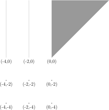
Figure 1: Fixed point set of the function $f$ of Example 3.1

Using Proposition 2.3, the semidifferential at $(0,0)$ is the function:

$$h\mapsto f^{\prime}_{(0,0)}(h_{1},h_{2})=(\max(\min(h_{1},h_{2}),0),\max(\max(h_{1},h_{2}),0)),$$

hence, $f^{\prime}_{(0,0)}$ vanishes on the nonpositive cone of $\mathbb{R}^{2}$ and so $f^{\prime}_{(0,0)}$ does not have any nonzero negative fixed point.

We just gave sufficient condition to the local minimality. Now, we give a sufficient condition to ensure that a fixed point is not the smallest one.

Proposition 3.2.

Suppose that $f$ is an order-preserving self-map and that the set $\{x\in\mathbb{R}^{d}\mid f(x)\leqslant x\}$ is bounded from below. Let $u$ be in ${\mathbf{Fix}}(f)$ and assume that $f$ is semidifferentiable at $u$. If ${\rho_{\mathbb{R}^{d}_{-}}(f^{\prime}_{u})}>1$ then $u$ is not the smallest fixed point.

Proof.

By definition of the spectral radius, ${\rho_{\mathbb{R}^{d}_{-}}(f^{\prime}_{u})}>1$ implies that, there exists $\mu>1$ and $h\in\mathbb{R}^{d}_{-}\backslash\{0\}$ such that, $f^{\prime}_{u}(h)=\mu h$. Let us write $\epsilon:=\displaystyle{\min_{h_{i}<0}-\mbox{$\|h\|$}^{-1}(\mu-1)h_{i}}>0$. There exists $t_{0}>0$ such that, $0<t<t_{0}$ implies that $f_{i}(u+th)\leqslant u_{i}+t\mu h_{i}+t\epsilon\mbox{$\|h\|$}$, for all $i$ such that $h_{i}<0$. Hence, for all $i$ such that $h_{i}<0$, $f_{i}(u+th)\leqslant u_{i}+t\mu h_{i}-t\mbox{$\|h\|$}^{-1}(\mu-1)h_{i}\mbox{$\|h\|$}=u_{i}+th_{i}<u_{i}$. Since $f$ is order-preserving, $f(u+th)\leqslant u$, for all $t\geqslant 0$, so $f_{i}(u+th)\leqslant u_{i}+th_{i}$, for all $i$ such that $h_{i}=0$.

We conclude that, $f(u+th)<u+th$. The sequence $(f^{k}(u+th))_{k\in\mathbb{N}}$ is nonincreasing and all its terms belong to the set $\{x\in\mathbb{R}^{d}\mid f(x)\leqslant x\}$ which is bounded from below, by continuity of $f$, it converges to a fixed point strictly smaller than $u$. ∎

Example 3.2.

We come back to Example 3.1. The map $f$ is clearly bounded from below since $f(x,y)\geqslant(-4,-4)$ for all $(x,y)\in\mathbb{R}^{2}$. We consider the fixed point $(0,-2)$. At this point, the semidifferential $f^{\prime}_{(0,-2)}$ is the function:

$$h\mapsto(0,\max(h_{1},0)+2h_{2}),$$

thus, $\rho_{\mathbb{R}_{-}^{2}}(f^{\prime}_{(0,-2)})=2$. By Theorem 3.2, $(0,-2)$ is not the smallest fixed point of $f$.

In Theorem 3.1 and Proposition 3.2, there are no restrictive conditions on the map. We next consider the special case of piecewise affine maps.

Proposition 3.3.

Let $f$ be a piecewise affine self-map on $\mathbb{R}^{d}$. There is neighborhood $\mathcal{V}$ of $u$ such that, for all $u+h\in\mathcal{V}$:

$$f(u+h)=f(u)+f^{\prime}_{u}(h)\enspace.$$

Proof.

Note that it is equivalent to show the equality for all coordinates of $f$ and we fix a coordinate $j\in\{1,\ldots,d\}$. We set, for all $a\in A_{j}$, $g_{a}(x)=\max_{b\in B_{a}}g_{a,b}(x)$. We denote by $\overline{B_{a}}$ the set of elements $b\in B_{a}$ such that $g_{a}(u)=g_{a,b}(u)$. There exists a neighborhood $\mathcal{V}_{a}$ of $u$ such that: $g_{a}(u+h)=\max_{b\in\overline{B_{a}}}g_{a,b}(u+h)$, for all $h$ such that $u+h\in\mathcal{V}_{a}$. Since $g_{a,b}$ is affine, we have: $g_{a,b}(u+h)=g_{a,b}(u)+\nabla g_{a,b}\cdot h$. It follows that, for all $\bar{b}\in\overline{B_{a}}$:

$$g_{a}(u+h)=g_{a,\bar{b}}(u)+\max_{b\in\overline{B_{a}}}\nabla g_{a,b}\cdot h$$ (1)

Let us denote $\overline{A_{j}}$ the set of elements $a\in A_{j}$ such that $f_{j}(u)=g_{a}(x)$. There exists a neighborhood of $u$, $\mathcal{V}\subseteq\bigcap_{a}\mathcal{V}_{a}$, such that: $f_{j}(u+h)=\min_{a\in\overline{A_{j}}}g_{a}(u+h)$ if $u+h\in\mathcal{V}$. Applying (1), we get: $f_{j}(u+h)=f_{j}(u)+\min_{a\in\overline{A_{j}}}\max_{b\in\overline{B_{a}}}\nabla g_{a,b}\cdot h$ if $u+h\in\mathcal{V}$. Clearly $h\mapsto\min_{a\in\overline{A_{j}}}\max_{b\in\overline{B_{a}}}\nabla g_{a,b}\cdot h$ is continuous and homogeneous thus it must coincide with the semidifferential of $f_{j}$ at $u$. Note that Proposition 2.3 follows from the latter fact. ∎

From Proposition 3.3, we deduce the following corollary which characterizes the locally minimal fixed point of piecewise affine maps.

Corollary 3.1.

Let $f$ be a piecewise affine self-map on $\mathbb{R}^{d}$ and let $u\in{\mathbf{Fix}}(f)$, then $u$ is a locally minimal fixed point if and only ${\mathbf{Fix}_{|\mathbb{R}^{d}_{-}}(f^{\prime}_{u})}=\{0\}$.

The second part of the previous proposition is the basis of a “descent” algorithm given in the section 4. If a fixed point $u$ is not locally minimal, then there exists a strictly negative fixed point $h$ for $f^{\prime}_{u}$ which may be thought of as a descent direction such that $u+h$ is a fixed point of $f$.

Example 3.3.

We consider the same example as before, Example 3.1. Now, we look at a fixed point of the form $z=(x,y)$ such that $y\geqslant x>0$. The map $f$ of Example 3.1 is piecewise affine. Following Proposition 2.3, at $z$ the semidifferential $f^{\prime}_{z}$ is the function:

$$h\mapsto\left\{\begin{array}[]{cc}(h_{1},h_{2})&\text{ if }y>x\\ (\min(h_{1},h_{2}),\max(h_{1},h_{2}))&\text{ if }y=x\end{array}\right.$$

In these two cases, $f^{\prime}_{z}$ admits a negative fixed point hence $z$ is not a locally fixed point. The isolated points of Figure 1 and the vector $(0,0)$ do not have any negative fixed point, we recover that these fixed points are locally minimal.

In order to pass from local minimality to global minimality, we shall need the following nonexpansiveness condition.

Definition 3.2 (Nonexpansive map).

Let $f$ be a self-map on $\mathbb{R}^{d}$: $f$ is nonexpansive (with respect to the sup-norm) if for all $x,y\in\mathbb{R}^{d}$, $\mbox{$\|f(x)-f(y)\|$}\leqslant\mbox{$\|x-y\|$}$.

Nonexpansiveness is automatically satisfied by Shapley operators since they are order-preserving and additively homogeneous.

Proposition 3.4.

Let $f$ be a nonexpansive self-map on $\mathbb{R}^{d}$ and let $u\in\mathbb{R}^{d}$. Assume that $f$ is semidifferentiable at $u$. Then ${\mathbf{Fix}_{|\mathbb{R}^{d}_{-}}(f^{\prime}_{u})}=\{0\}$ if and only if ${\rho_{\mathbb{R}^{d}_{-}}(f^{\prime}_{u})}<1$.

Proof.

It suffices to show that ${\rho_{\mathbb{R}^{d}_{-}}(f^{\prime}_{u})}\leqslant 1$. Firstly, $f^{\prime}_{u}$ is nonexpansive as a pointwise limit of nonexpansive maps. Assume that ${\rho_{\mathbb{R}^{d}_{-}}(f^{\prime}_{u})}>1$, there exists $\mu>1$ and $v\in\mathbb{R}^{d}_{-}$ such that $f^{\prime}_{u}(v)=\mu v$, then $\mbox{$\|f^{\prime}_{u}(v)-f^{\prime}_{u}(0)\|$}=\mu\mbox{$\|v\|$}>\mbox{$\|v-0\|$}$ which contradicts the nonexpansiveness of $f^{\prime}_{u}$. ∎

The main result of this paper is the following theorem, which will allow us to check the global minimality of a fixed point.

Theorem 3.2.

Let $f$ be an order-preserving nonexpansive self-map on $\mathbb{R}^{d}$. Let $u$ be a fixed point of $f$. Then, $u$ is locally minimal if and only if it is the smallest fixed point of $f$. If in addition $f$ is piecewise affine, the following assertions are equivalent:

1. $u$ is the smallest fixed point of $f$.

2. ${\mathbf{Fix}_{|\mathbb{R}^{d}_{-}}(f^{\prime}_{u})}=\{0\}$.

3. ${\rho_{\mathbb{R}^{d}_{-}}(f^{\prime}_{u})}<1$.

The proof of this theorem relies on the existence of an order-preserving and nonexpansive retract on the fixed point set of $f$. This idea was already used in [CGG⁺05]. The existence of nonexpansive retracts on the fixed point set is a classical topic in the theory of nonexpansive mappings, see Nussbaum [Nus88]. In the present finite dimensional case, the result of the next lemma is an elementary one.

Lemma 3.1.

Let $f$ be a nonexpansive order-preserving self-map on $\mathbb{R}^{d}$. Let $u$ be in ${\mathbf{Fix}}(f)$. Then there is a nonlinear order-preserving and nonexpansive map $P$ such that $P(\mathbb{R}^{d})={\mathbf{Fix}}(f)$ and $\mathbf{Fix}(P)={\mathbf{Fix}}(f)$.

Proof.

Following the idea of [GG04], we shall construct the map $P$ as follow: $P(x)=\lim_{k\to+\infty}f^{k}(y)$ where $y=\limsup_{l\to+\infty}f^{l}(x)$. Since $f$ is nonexpansive and $u\in{\mathbf{Fix}}(f)$, $(f^{k}(x))_{k\in\mathbb{N}}$ is bounded for all $x\in\mathbb{R}^{d}$. We can now write, for all $x\in\mathbb{R}^{d}$, $Q(x)=\limsup_{k\to+\infty}f^{k}(x)$. Moreover, given $k\geqslant 0$, we have, for all $m\geqslant k$, $\sup_{n\geqslant k}f^{n}(x)\geqslant f^{m}(x)$ and since $f$ is order-preserving, for all $m\geqslant k$, $f(\sup_{n\geqslant k}f^{n}(x))\geqslant f(f^{m}(x))$ so, $f(\sup_{n\geqslant k}f^{n}(x))\geqslant\sup_{m\geqslant k}f(f^{m}(x))$, we conclude, by taking the limit when $k$ tends to $+\infty$ and using the continuity of $f$, $f(Q(x))\geqslant Q(x)$, so $(f^{l}(Q(x))_{k\in\mathbb{N}}$ is a nondecreasing sequence. Moreover, since $f$ is nonexpansive, the limit $P(x)=\lim_{l\to+\infty}f^{l}(Q(x))$ is finite. Observe that the map $P$ is order-preserving and nonexpansive since it is the pointwise limit of order-preserving and nonexpansive maps. Furthermore, $f(P(x))=f(\lim f^{l}(Q(x))=\lim f^{l+1}Q(x)=P(x)$ so $P(\mathbb{R}^{d})\subseteq{\mathbf{Fix}}(f)$. Moreover, it is easy to see that $P$ fixes every fixed point of $f$. It follows that $P$ is a projector. ∎

Proof of Theorem 3.2.

Suppose that $u$ is a locally minimal fixed point but not the smallest fixed point. Then, there is a fixed point $v$ such that $\inf(v,u)<u$. For all scalars $t\geqslant 0$, define $\omega_{t}:=\inf(v+t,u)$. Let us take $P$ as in Lemma 3.1. Since $P$ is nonexpansive in the sup-norm, $\mbox{$\|P(v+t)-P(v)\|$}\leqslant t$ for all $t\geqslant 0$ and so $P(v+t)\leqslant P(v)+t$. Using the monotonicity of $P$, we deduce that $P(\omega_{t})\leqslant\inf(P(v+t),P(u))\leqslant\inf(P(v)+t,P(u))=\omega_{t}$. Let $t_{0}=\inf\{t\geqslant 0\mid\omega_{t}=u\}$. Then, for $0<t<t_{0}$, $P(\omega_{t})$ is a fixed point of $f$, which is such that $P(\omega_{t})<u$. Since $P$ is continuous, $P(\omega_{t})$ tends to $P(\omega_{t_{0}})=P(u)=u$ as $t$ tends to $t_{0}^{-}$, which contradicts the local minimality of $u$. Hence a contradiction with $u$ not being the smallest fixed point. Define by $1^{\prime}$ the property that $u$ is a locally minimal fixed point. We just showed $1\Leftrightarrow 1^{\prime}$. By Theorem 3.1, we get $3\implies 2\implies 1^{\prime}$. By Corollary 3.1, $1^{\prime}\implies 2$ and by Proposition 3.4 we get $2\implies 3$. ∎

4 A policy iteration algorithm to compute the smallest fixed point

The previous results justify the following policy iteration algorithm which returns the smallest fixed point of a nonexpansive order-preserving piecewise affine map. Assume that $f$ is a map from $\mathbb{R}^{d}$ to $\mathbb{R}^{d}$, every coordinate of which is given by

$$f_{j}(x)=\inf_{a\in A_{j}}f^{a}(x)$$ (2)

where $A_{j}$ is finite and every $f_{a}$ is a supremum of order-preserving nonexpansive affine maps. A strategy $\pi$ is a map from $\{1,\cdots,d\}$ to $\mathcal{A}=\bigcup_{1\leqslant j\leqslant d}A_{j}$ such that $\pi(j)\in A_{j}$ for all $j$. We define $f^{\pi}=(f^{\pi(1)},\cdots,f^{\pi(j)},\cdots,f^{\pi(d)})$. We assume that every map $f^{\pi}$ has a smallest fixed point. The idea of the algorithm is to use a descent direction to select the new strategy when a non-minimal fixed point is reached . The algorithm, needs two oracles. Oracle 1 returns the smallest fixed point in $\mathbb{R}^{d}$ of a map $f^{\pi}$. Oracle 2 checks whether the restriction of $f^{\prime}_{u}$ to the convex cone $\mathbb{R}^{d}_{-}$ has a spectral radius equal to 1, and if this is the case, returns a vector $h\in\mathbb{R}^{d}_{-}\backslash\{0\}$ such that $f^{\prime}_{u}(h)=h$. We discuss below the implementation of these oracles for subclasses of maps.

Algorithm 1 Computing the smallest fixed point by Policy Iteration

Input: An order-preserving nonexpansive map $f$ in the form (2).
Output: The smallest fixed point of $f$ in $\mathbb{R}^{d}$.
Init: Select a strategy $\pi^{0}$, $k=0$.
Value Determination $\mathbf{(D_{k})}$: Call Oracle 1 to compute the smallest fixed point $u^{k}$ of $f^{\pi^{k}}$ in $\mathbb{R}^{d}$.
Policy Improvement $\mathbf{(I_{k}^{1})}$: If $f(u^{k})<u^{k}$, take $\pi^{k+1}$ such that $f(u^{k})=f^{\pi^{k+1}}(u^{k})$ and go to Step $\mathbf{(D_{k+1})}$.
Policy Improvement $\mathbf{(I_{k}^{2})}$: If $f(u^{k})=u^{k}$, call Oracle 2 to compute $\alpha_{k}:=\rho(f_{u^{k}}^{\prime})$.

$\bullet$ If $\alpha_{k}<1$, return $u^{k}$, which is the smallest fixed point of $f$.

$\bullet$ If $\alpha_{k}=1$, take $h\in\mathbb{R}^{d}_{-}\backslash\{0\}$ such that $f_{u^{k}}^{\prime}(h)=h$. Define $\pi^{k+1}(j)$ as an optimal action $a$ in $(f_{u^{k}}^{\prime})_{j}(h)=\min_{a\in\overline{A_{j}}}(f^{a})^{\prime}_{u^{k}}(h)$ where $\overline{A_{j}}=\{a\in A_{j}\mid f^{a}(u^{k})=f_{j}(u^{k})\}$. Then go to $\mathbf{(D_{k+1})}$.

Since the number of strategies is finite, we shall see that the existence of a smallest fixed point in $\mathbb{R}^{d}$ for every policy suffices to show that Algorithm 1 terminates. We start by proving that the smallest fixed point of a nonexpansive and order-preserving self-map on $\mathbb{R}^{d}$ can be computed using an optimization problem.

Proposition 4.1.

Let $g$ be an order-preserving nonexpansive self-map on $\mathbb{R}^{d}$. Assume that $g$ has a smallest fixed point in $\mathbb{R}^{d}$ denoted by $u$.

1. The vector $u$ is the smallest element of $\{x\in\mathbb{R}^{d}\mid g(x)\leqslant x\}$;

2. The vector $u$ is the unique optimal solution of the minimization problem: $\min\{\sum_{1\leqslant i\leqslant d}x_{i}\mid x\in\mathbb{R}^{d},\ g(x)\leqslant x\}$.

Proof.

The vector $u$ satisfies $g(u)=u$ and a fortiori $g(u)\leqslant u$. Let $x$ be any vector satisfying $g(x)\leqslant x$. Since $g$ is order-preserving, nonexpansive and has a fixed point, $(g^{k}(x))_{k\in\mathbb{N}}$ is a bounded nonincreasing sequence. Denoting by $y$ the limit of $(g^{k}(x))_{k\in\mathbb{N}}$, we get $y\leqslant x$ and $y$ is a finite fixed point of $g$ so $y\geqslant u$, the first assertion is thus proved. We conclude next that $\sum_{1\leqslant i\leqslant d}u_{i}\leqslant\sum_{1\leqslant i\leqslant d}y_{i}\leqslant\sum_{1\leqslant i\leqslant d}x_{i}$. Since this holds for all feasible $x$, it follows that $u$ is an optimal solution. If $x$ is an arbitrary optimal solution, we must have $\sum_{1\leqslant i\leqslant d}u_{i}=\sum_{1\leqslant i\leqslant d}x_{i}$ and since $u\leqslant x$, it follows that $u=x$ and the second assertion is proved. ∎

Now, we prove that Algorithm 1 terminates when policies have a smallest fixed point.

Theorem 4.1 (Termination of Algorithm 1).

Let $f$ be an order-preserving nonexpansive map in the form (2). If every policy $f^{\pi}$ has a smallest fixed point in $\mathbb{R}^{d}$, then Algorithm 1 terminates.

Proof.

To show that Algorithm 1 terminates, it suffices to check that the sequence of produced points $u^{0},u^{1},\cdots$ is strictly decreasing, because the corresponding policies must be distinct and the number of policies is finite. Let $k$ be an integer. Let be $u^{k}$ be a vector of $\mathbb{R}^{d}$. Suppose that an improvement of type $I_{k}^{1}$ arises: $f(u^{k})<u^{k}$. There exists a policy $f^{\pi^{k+1}}$ such that $f^{\pi^{k+1}}(u^{k})=f(u^{k})$. Let us denote $u^{k+1}$ the smallest fixed point of $f^{\pi^{k+1}}$. Since $u^{k}$ belongs to the set $\{x\in\mathbb{R}^{d}\mid f^{\pi^{k+1}}(x)\leqslant x\}$, we conclude from the first assertion of Proposition 4.1 that $u^{k+1}\leqslant u^{k}$. Furthermore, since $u^{k}$ is not a fixed point of $f^{\pi^{k+1}}$, $u^{k+1}<u^{k}$. Suppose that an improvement of type $I_{k}^{2}$ arises: $u^{k}$ is not the smallest fixed point of $f$. Then, since $f$ is piecewise affine and nonexpansive, by Proposition 3.1 and Theorem 3.2, there exists $h\in\mathbb{R}^{d}_{-}\backslash\{0\}$, $f^{\pi^{k+1}}(u^{k}+th)=u^{k}+th$ for $t>0$ small enough. It follows that $u^{k+1}\leqslant u^{k}+th<u^{k}$. ∎

Now, we discuss the implementation of the oracles. Using Proposition 4.1 assertion 2, the following corollary identifies a situation where Oracle 1 can be implemented by solving a linear programming problem.

Corollary 4.1.

Let $g$ be an order-preserving nonexpansive map that is the supremum of finitely many affine maps. Assume, that $g$ has a smallest fixed point $u$ in $\mathbb{R}^{d}$. Then $u$ is the unique optimal solution of the linear program:

$$\min\{\sum_{1\leqslant i\leqslant d}x_{i}\mid x\in\mathbb{R}^{d},\ g(x)\leqslant x\}.$$

The implementation of Oracle 2 raises the issue of computing the spectral radius. Let $g$ be an order-preserving, homogeneous and continuous self-map of $\mathbb{R}^{d}_{-}$. It is known that:

$$\rho_{\mathbb{R}^{d}_{-}}(g) =\inf_{x\in\operatorname{int}(\mathbb{R}^{d}_{-})}\sup_{1\leqslant i\leqslant d}\frac{g_{i}(x)}{x_{i}}$$ (3)

$$\rho_{\mathbb{R}^{d}_{-}}(g) =\sup_{x\in\mathbf{\mathbb{R}^{d}_{-}}}\limsup_{k\to+\infty}\mbox{$\|g^{k}(x)\|$}^{\frac{1}{k}}$$ (4)

The first equality, which is a generalization of the Collatz-Wielandt property in Perron-Frobenius theory, follows from a result of Nussbaum [Nus86] Theorem 3.1. The second characterization is shown by Mallet-Paret and Nussbaum in [MPN02] under more general assumptions. We deduce, for every vector $x\in\operatorname{int}(\mathbb{R}^{d}_{-})$:

$$\rho_{\mathbb{R}^{d}_{-}}(g)\leqslant\left(\sup_{1\leqslant i\leqslant d}\frac{g_{i}^{k}(x)}{x_{i}}\right)^{\frac{1}{k}}.$$ (5)

Moreover, the latter upper bound converges to $\rho_{\mathbb{R}^{d}_{-}}(g)$ as $k$ tends to infinity. This yields an obvious method to check whether $\rho_{\mathbb{R}^{d}_{-}}(g)<1$, which consists in computing the upper bound in (5) for successive values of $k$ as long as the upper bound is not smaller than 1. This algorithm will not stop when $\rho_{\mathbb{R}^{d}_{-}}(g)=1$. However, we next describe simple situations where this idea leads to a terminating algorithm.

First, we can adapt Proposition 4.1 to compute a descent direction from a linear program when the semidifferential coincides with a supremum of finitely many affine maps. Since the semidifferential is a homogeneous map we can add box constraints to the linear program of Proposition 4.1. From now, we denote $\mathbf{e}$ the vector the coordinates of which are equal to $-1$.

Proposition 4.2.

Let $g$ be a homogeneous order-preserving nonexpansive self-map. Assume, that the restriction of $g$ on the nonpositive cone $\mathbb{R}^{d}_{-}$ is the supremum of finitely many affine maps. Let $\alpha$ be a nonnegative real number. The unique optimal solution of the linear program:

$$\min\left\{\sum_{1\leqslant i\leqslant d}x_{i}\mid x\in\mathbb{R}^{d},\ g(x)\leqslant x,\ \alpha\mathbf{e}\leqslant x\leqslant 0\right\} P_{\alpha}$$ ()

is the smallest fixed point of $g$ in the set $\{x\in\mathbb{R}^{d}\mid\alpha\mathbf{e}\leqslant x\leqslant 0\}$.

Furthermore, if there exists $\alpha>0$ such that the optimal value of ($P_{\alpha}$) is equal to 0 then the null vector is the unique fixed point of $g$ in $\mathbb{R}^{d}_{-}$.

Proof.

Since $g$ is nonexpansive and homogeneous, $\mbox{$\|g(\alpha\mathbf{e})\|$}\leq\alpha$ and thus $g(\alpha\mathbf{e})\geqslant\alpha\mathbf{e}$. Moreover, $g$ is order-preserving, we conclude that $g$ is a self-map on $\{x\in\mathbb{R}^{d}\mid\alpha\mathbf{e}\leqslant x\leqslant 0\}$ which is a complete lattice. From Tarski’s theorem, $g$ has a smallest fixed point $u$ such that $\alpha\mathbf{e}\leqslant u\leqslant 0$ and $u$ is the smallest element of the feasible set of ($P_{\alpha}$). Using the same argument as in assertion 2 of Proposition 4.1, we conclude that $u$ is the unique optimal solution of ($P_{\alpha}$).

Now, suppose there exists $\alpha>0$ such that the optimal value of ($P_{\alpha}$) is 0 and assume that $g$ has a nonzero fixed point $u$ in $\mathbb{R}^{d}_{-}$. Since $g$ is homogeneous, $\alpha u/\mbox{$\|u\|$}$ is a feasible point of ($P_{\alpha}$), the sum of coordinates of this vector is strictly smaller than 0 which contradicts the fact that 0 is the optimal value of ($P_{\alpha}$). ∎

The second simple case concerns the homogeneous min-max functions.

Definition 4.1.

We call a homogeneous min-max function of the variables $h_{1},\ldots,h_{d}$ a term in the grammar: $X\mapsto\min(X,X),\max(X,X),h_{1},\cdots,h_{d},0$.

For instance, the term $\min(h_{1},\max(h_{2},h_{3},0))$ is produced by this grammar. More generally, we shall say that a map from $\mathbb{R}^{d}$ to $\mathbb{R}^{d}$ is a homogeneous min-max self-map if its coordinates are of the form of Definition 4.1. This definition is inspired by the min-max functions considered by Gunawardena [Gun94] and Olsder [Ols91]. The terms of this form comprise the semidifferentials of the min-max functions considered there. For simple classes of programs, like the one we shall consider in the next section, the semidifferential at any fixed point turns out to be a homogeneous min-max function. In this case, the spectral radius can be computed efficiently by using to the following integrity argument $g(\mathbb{Z}^{d})\subseteq\mathbb{Z}^{d}$.

Proposition 4.3.

Let $g$ be a homogeneous min-max self-map on $\mathbb{R}^{d}$. Then $\rho_{\mathbb{R}^{d}_{-}}(g)\in\{0,1\}$. Moreover $\rho_{\mathbb{R}^{d}_{-}}(g)=0$ if and only if $\lim_{k\to+\infty}g^{k}(\mathbf{e})=0$, and the latter limit is reached in at most $d$ steps.

Proof.

Since $g$ is nonexpansive and $g(0)=0$, we have $g(\mathbf{e})\geqslant\mathbf{e}$. We deduce, by monotonicity of $g$, that $(g^{k}(\mathbf{e}))_{k\in\mathbb{N}}$ is a nondecreasing sequence bounded from above by 0. Moreover, $g$ preserves the set of integer vectors. So this sequence converges in at most $d$ steps to some vector $b\in\mathbb{Z}_{-}^{d}$. Let us suppose that $b=0$. For all $y\in\mathbb{R}^{d}_{-}$, there exists $t\geqslant 0$ such that, $0\geqslant y\geqslant t\mathbf{e}$. Since $g$ is homogeneous and order-preserving, $0\geqslant g^{k}(y)\geqslant tg^{k}(\mathbf{e})=0$ for all $k\geqslant d$ which implies that $\rho_{\mathbb{R}^{d}_{-}}(g)=0$. If $b<0$ we have $g(b)=b\neq 0$, and so $\rho_{\mathbb{R}^{d}_{-}}(g)\geqslant 1$. Finally, since $g$ is nonexpansive, we also have $\rho_{\mathbb{R}^{d}_{-}}(g)\leqslant 1$. ∎

5 Applications

5.1 Applications to positive stochastic games

In this subsection, we consider applications to game theory, particularly in zero-sum positive stochastic games. The term ”positive” means that all the rewards are nonnegative. We are interested in the expectation of the infinite sum of rewards at each date without discounting. Filar and Vrieze [FV97, Theorem 4.4.3] prove that the value of a positive stochastic game is the smallest nonnegative fixed point of a Shapley operator. They also develop a value iteration [FV97, Theorem 4.4.4] to compute the value of this class of games. Although value iteration is generally an effective method, one can construct examples in which policy iteration is much faster. This occurs when the contraction rate of value iteration is close to one, or when the initial estimate of the value function is too far away from the true value function. We give such an example in Example 5.1. In consequence, we propose to use Algorithm 1 to compute the value of zero-sum positive stochastic game with perfect information.

Example 5.1.

Let us consider the positive game in perfect information with three states represented by Figure 2. The real $\epsilon$ is chosen in $(0,1/2]$. In the game the two players can stop the game at each state they can play. The diamond node (state 1) is a stochastic node, the circle node (state 2) is controlled by $MIN$ and the triangle node (state 3) is controlled by $MAX$. The thick edges represent the deterministic transitions, whereas dotted ones represent stochastic transitions. The double octagons are the stopping options for each player and the numbers inside are stopping payoffs. The numbers on the edges are either immediate payoffs if the nodes are controlled by players, or the probability to reach the state at the endpoint of the edge.

Figure 2: The game of Example 5.1

The dynamic operator $f_{\varepsilon}$ is thus defined as the following function:

$$f_{\varepsilon}(x)=f_{\varepsilon}\left(\begin{array}[]{c}x_{1}\\ x_{2}\\ x_{3}\end{array}\right)=\left(\begin{array}[]{ccc}(1-\varepsilon)x_{2}+\varepsilon x_{3}\\ \min(x_{1}+\dfrac{\varepsilon}{2},x_{2}+\dfrac{\varepsilon}{2},x_{3}+\varepsilon^{2},\varepsilon^{-1})\\ \max(x_{1}+\sqrt{\varepsilon},x_{2}+\varepsilon^{2},x_{3},\varepsilon^{-2})\\ \end{array}\right)$$

Since $\varepsilon\in(0,1/2]$, the value of the game is $V_{\varepsilon}=(2\varepsilon^{-1}-1,\varepsilon^{-1},\varepsilon^{-2})$. Indeed, $V_{\varepsilon}$ is a fixed point of $f_{\varepsilon}$ and the semidifferential at $V_{\epsilon}$ is the following map: $(h_{1},h_{2},h_{3})\mapsto((1-\varepsilon)h_{2}+\varepsilon h_{3},0,\max(h_{3},0))$ which only admits $(0,0,0)$ as nonpositive fixed point and using Theorem 3.2, we conclude that $V_{\epsilon}$ is the smallest (positive) fixed point of $f_{\varepsilon}$ and thus the value of the game. An optimal policy is given by selecting the stopping options for each player. Since we chose these stopping options as initial policy (this is our heuristic choice for the next examples), policy iteration algorithm does not need any further iteration to converge.

Table 1 shows the numbers of iterations needed by the value iteration (VI) for different values of $\varepsilon$. The value iteration is initialized with the null vector $(0,0,0)$ and stops when the $\ell_{\infty}$ norm of the difference between two iterates are smaller than $10^{-6}$.

$\varepsilon$	# iterations for VI
0.5	11
0.25	35
0.1	203
0.01	200,003
0.001	2,000,003

Table 1: Numbers of iterations for Value Iteration for different values of $\varepsilon$

5.1.1 A detailed example of a positive game in perfect information

As in Example 5.1, we consider a positive stochastic games with stopping options. Again the space of states are decomposed in three kinds of states: the states controlled by $MIN$, the ones controlled by $MAX$ and the stochastic states. The graph depicted by Figure 3 represents the game. The circle states are controlled by $MIN$, the triangle ones by $MAX$ and the diamond ones are the stochastic states. The other nodes (represented by double octagons) are the stopping options and the numbers inside represent the payoff. For the nodes controlled by the players, the thick edges are the different actions for the players and the numbers on them are the immediate payoff. The dotted edges are the different transitions from a stochastic state to other states.

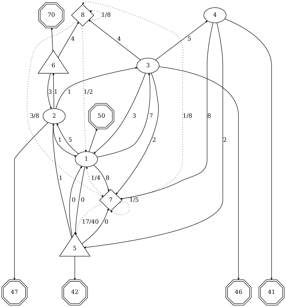
Figure 3: The graph associated of the dynamic operator

The Shapley operator for this game is given by the following order-preserving piecewise affine nonexpansive map:

$$f(x)=f\left(\begin{array}[]{c}x_{1}\\ x_{2}\\ x_{3}\\ x_{4}\\ x_{5}\\ x_{6}\\ x_{7}\\ x_{8}\end{array}\right)=\left(\begin{array}[]{ccc}\min(x_{2}+5,x_{3}+7,x_{5},x_{7}+8,50)\\ \min(x_{1}+1,x_{3}+1,x_{6}+1,47)\\ \min(x_{1}+3,x_{4}+5,x_{7}+2,x_{8}+4,46)\\ \min(x_{5}+2,x_{7}+8,41)\\ \max(x_{1},x_{2}+1,x_{7},42)\\ \max(x_{2}+3,x_{8}+4,70)\\ (1/4)x_{1}+(17/40)x_{5}+(1/5)x_{7}+(1/8)x_{8}\\ (1/2)x_{1}+(3/8)x_{7}+(1/8)x_{8}\end{array}\right)$$

We can compute the value of the game by value iteration, it takes 42 iterations. Here, we apply Algorithm 1 to compute the smallest nonnegative fixed point of $f$ which determines the value of the game. To do this we can use a map $\tilde{f}$ which coincides with the Shapley operator $f$ on the nonnegative cone and the fixed point of which are nonnegative. To construct $\tilde{f}$, it suffices to replace for the states controlled by $MIN$ and the stochastic states, the linear forms $a\cdot x+b_{i}$ by $\max(a\cdot x+b_{i},0)$. Now, we initialize (Step $\mathbf{(D_{0})}$) Algorithm 1 by taking the stopping options. We get the following map $\tilde{f}^{0}$:

$$\tilde{f}^{\pi^{0}}(x)=\left(\begin{array}[]{ccc}50\\ 47\\ 46\\ 41\\ \max(x_{1},x_{2}+1,x_{7},42)\\ \max(x_{2}+3,x_{8}+4,70)\\ \max((1/4)x_{1}+(17/40)x_{5}+(1/5)x_{7}+(1/8)x_{8},0)\\ \max((1/2)x_{1}+(3/8)x_{7}+(1/8)x_{8},0)\end{array}\right)$$

By a linear program (Proposition 4.1), we compute the smallest fixed point of $\tilde{f}^{\pi^{0}}$, we find the vector $\bar{x}=(50,47,46,41,50,70,50,50)^{\intercal}$. As required by step $\mathbf{(I_{0}^{1})}$, we have to check whether $\bar{x}$ is fixed point of $\tilde{f}$, this is the case. Now we enter in step $\mathbf{(I_{1}^{1})}$, to check whether $\bar{x}$ is the smallest fixed point of $\tilde{f}$, we compute the semidifferential of $\tilde{f}$ at $\bar{x}$ in the direction $h$ using Proposition 2.3, we obtain the map $\tilde{f}^{\prime}_{\bar{x}}$ defined as follows:

$$\left(\begin{array}[]{ccc}\min(h_{5},0)\\ \min(h_{3},0)\\ \min(h_{4},0)\\ 0\\ \max(h_{1},h_{7})\\ 0\\ (1/4)h_{1}+(17/40)h_{5}+(1/5)h_{7}+(1/8)h_{8}\\ (1/2)h_{1}+(3/8)h_{7}+(1/8)h_{8}\end{array}\right)$$

On the nonpositive cone, the components of $\tilde{f}^{\prime}_{\bar{x}}$ are linear forms except for the sixth component which is a maximum of linear forms. Then, we can use Proposition 4.2 as Oracle 2 to determine whether $\bar{x}$ is the smallest fixed point of $\tilde{f}$. The unique optimal solution of linear program $\min\{\sum_{j}h_{j}\mid\tilde{f}^{\prime}_{\bar{x}}(h)\leqslant h,h_{i}\in[-1,0],\ \forall i\}$ is $\bar{h}=(-1,0,0,0,-1,0,-1,-1)^{\intercal}$. We use this vector as descent direction. The vector $\bar{h}$ gives us a new policy which is:

$$\tilde{f}^{\pi^{1}}(x)=\left(\begin{array}[]{ccc}x_{5}\\ 47\\ 46\\ 41\\ \max(x_{1},x_{2}+1,x_{7},42)\\ \max(x_{2}+3,x_{8}+4,70)\\ (1/4)x_{1}+(17/40)x_{5}+(1/5)x_{7}+(1/8)x_{8}\\ (1/2)x_{1}+(3/8)x_{7}+(1/8)x_{8}\end{array}\right)$$

and we go to the step $\mathbf{(D_{1})}$. By a linear program (Proposition 4.1), we compute the smallest fixed point of $\tilde{f}^{\pi^{1}}$, we find the vector $x^{*}=(48,47,46,41,48,$ $70,48,48)^{\intercal}$. The vector $x^{*}$ is also a fixed point of $\tilde{f}$. We enter in the step $\mathbf{(I_{1}^{1})}$. We compute the semidifferential of $\tilde{f}$ at $x^{*}$ in the direction $h$ using Proposition 2.3, we obtain the map $\tilde{f}^{\prime}_{x^{*}}$ defined as follows:

$$\hskip 28.45274pt\left(\begin{array}[]{ccc}\min(h_{5},0)\\ \min(h_{3},0)\\ \min(h_{4},0)\\ 0\\ \max(h_{1},h_{2},h_{7})\\ 0\\ (1/4)h_{1}+(17/40)h_{5}+(1/5)h_{7}+(1/8)h_{8}\\ (1/2)h_{1}+(3/8)h_{7}+(1/8)h_{8}\end{array}\right)$$

To check whether $x^{*}$ is the smallest fixed point of $\tilde{f}$, we can proceed by computing the upper bound of Equation (5) where $g$ is the semidifferential of $\tilde{f}$ at $x^{*}$. Taking the vector $e$ the coordinates of which are equal to $-1$, we find that $\max_{1\leqslant i\leqslant 8}\dfrac{g_{i}^{6}(e)}{e_{i}}=\dfrac{109}{320}<1$ and we conclude that $x^{*}$ is the smallest fixed point of $\tilde{f}$ and so the value of the game depicted by Figure 3.

Remark 5.1.

We could also use the same linear program ($P_{\alpha}$) with $\alpha=1$. In the case of the semidifferential of $\tilde{f}$ at $x^{*}$, the optimal value would be equal to zero and the unique optimal solution would be the null vector.

5.2 Applications to static analysis of programs

We next illustrate our results on an example from static analysis. We take a simple but interesting program with nested loops (Figure 5). From this program, we create semantic equations on the lattice of intervals [CC77] (Figure 5) that describe the outer approximations of the sets of values that program variables can take, for all possible executions. For instance, at control point 4, the value of variable $y$ can come either from point 3 or point 5 (hence the union operator), as long as the condition $y\geqslant 5$ is satisfied (hence the intersection operator). An interval $I$ is written as $[-i^{-},i^{+}]$ in order to get fixed point equations of order-preserving maps in $i^{i}$ and $i^{+}$. The equations we derive on bounds are order-preserving piecewise affine maps, to which we can apply our methods.

int x,int y,
x=[0,2];y=[10,15]	//1
while (x<=y) {	//2
x=x+1;	//3
while (5<=y) {	//4
y=y-1;	//5
}	//6
}	//7

Figure 4: A simple C program

$$(x_{1},y_{1}) = ([0,2],[10,15])$$

$$x_{2} = (x_{1}\cup x_{6})\cap[-\infty,(y_{1}\cup y_{6})^{+}]$$

$$y_{2} = (y_{1}\cup y_{6})\cap[(x_{1}\cup x_{6})^{-},+\infty]$$

$$(x_{3},y_{3}) = (x_{2}+[1,1],y_{2})$$

$$(x_{4},y_{4}) = (x_{3},(y_{3}\cup y_{5})\cap[5,+\infty])$$

$$(x_{5},y_{5}) = (x_{4},y_{4}+[-1,-1])$$

$$(x_{6},y_{6}) = (x_{5},(y_{3}\cup y_{5})\cap[-\infty,4])$$

$$x_{7} = (x_{1}\cup x_{6})\cap[(y_{1}\cup y_{6})^{-}+1,+\infty]$$

$$y_{7} = (y_{1}\cup y_{6})\cap[-\infty,(x_{1}\cup x_{6})^{+}-1]$$

Figure 5: Its abstract semantic equations in intervals

The order-preserving nonexpansive piecewise affine map $f$ for the bounds of these intervals is:

$$f\left(\begin{array}[]{c}x\\ y\end{array}\right)=f\left(\begin{array}[]{c}x_{2}^{-}\\ x_{2}^{+}\\ x_{7}^{-}\\ x_{7}^{+}\\ y_{2}^{-}\\ y_{2}^{+}\\ y_{4}^{-}\\ y_{4}^{+}\\ y_{6}^{-}\\ y_{6}^{+}\\ y_{7}^{-}\\ y_{7}^{+}\end{array}\right)=\left(\begin{array}[]{ccc}0&\vee&(x_{2}^{-}-1)\\ 2\vee(x_{2}^{+}+1)&\wedge&\underline{15\vee y_{6}^{+}}\\ 0\vee(x_{2}^{-}-1)&\wedge&\underline{(-10\vee y_{6}^{-})-1}\\ 0&\vee&(x_{2}^{+}+1)\\ \underline{0\vee(x_{2}^{-}-1)}&\wedge&-10\vee y_{6}^{-}\\ 15&\vee&y_{6}^{+}\\ y_{2}^{-}\vee(y_{4}^{-}+1)&\wedge&\underline{-5}\\ y_{2}^{+}&\vee&y_{4}^{+}-1\\ y_{2}^{-}&\vee&y_{4}^{-}+1\\ y_{2}^{+}\vee(y_{4}^{+}-1)&\wedge&\underline{4}\\ -10&\vee&y_{6}^{-}\\ 15\vee y_{6}^{+}&\wedge&\underline{(2\vee(x_{2}^{+}+1))-1}\end{array}\right)$$

In the equations for the intervals $x_{2},y_{2},y_{4},y_{6},x_{7}$ and $y_{7}$, an intersection appears, which gives a $\min$ ($\wedge$) in the corresponding coordinate of $f$. Choosing a policy is the same as replacing every minimum of terms by one of the terms, which yields a simpler “minimum-free” nonlinear map, which can be interpreted as the dynamic programming operator of a one-player problem.

We next illustrate Algorithm 1. The underlined terms in the expression of $f$ indicate the initial policy $\pi^{0}$, for instance, the fifth coordinate of $f^{\pi^{0}}$ is $0\vee(x_{2}^{-}-1)$. We first compute the smallest fixed point of this policy (Step $\mathbf{(D_{0})}$). This may be done by linear programming (Proposition 4.1), or, in this special case, by a reduction to a shortest path problem. We find $(\bar{x},\bar{y})=(0,15,-1,16,0,15,-5,15,0,4,0,15)^{\intercal}$. The first Policy Improvement step, $\mathbf{(I^{1}_{0})}$, requires to check whether this is a fixed point of $f$. This turns out to be the case. To determine whether $(\bar{x},\bar{y})$ is actually the smallest fixed point, we enter in the second policy improvement step, $\mathbf{(I^{2}_{0})}$. We calculate the semidifferential at $(\bar{x},\bar{y})$ in the direction $(\delta x,\delta y)$, using Proposition 2.3:

$$\begin{array}[]{rcl}f^{\prime}_{(\bar{x},\bar{y})}\left(\delta\bar{x},\delta\bar{y}\right)^{\intercal}&=&\left(0,0,\delta\bar{y}_{6}^{-},\delta\bar{x}_{2}^{+},0\wedge\delta\bar{y}_{6}^{-},0,0,\delta\bar{y}_{2}^{+},\delta\bar{y}_{2}^{-},0,\delta\bar{y}_{6}^{-},0\wedge\delta\bar{x}_{2}^{+}\right)^{\intercal}\end{array}$$

The method of Proposition 4.3, which we use as Oracle 2, yields in three steps a fixed point for $f^{\prime}_{(\bar{x},\bar{y})}$ that we denote by $h=(0,0,-1,0,-1,0,0,0,-1,0,-1,0)^{\intercal}$. This fixed point determines the new policy $\pi^{1}$, which corresponds to the map $g:=f^{\pi^{1}}$ given by:

$$g\left(\begin{array}[]{c}x\\ y\end{array}\right)=g\left(\begin{array}[]{c}x_{2}^{-}\\ x_{2}^{+}\\ x_{7}^{-}\\ x_{7}^{+}\\ y_{2}^{-}\\ y_{2}^{+}\\ y_{4}^{-}\\ y_{4}^{+}\\ y_{6}^{-}\\ y_{6}^{+}\\ y_{7}^{-}\\ y_{7}^{+}\end{array}\right)=\left(\begin{array}[]{ccc}0&\vee&x_{2}^{-}-1\\ 15&\vee&y_{6}^{+}\\ -11&\vee&y_{6}^{-}-1\\ 0&\vee&x_{2}^{+}+1\\ -10&\vee&y_{6}^{-}\\ 15&\vee&y_{6}^{+}\\ &-5&\\ y_{2}^{+}&\vee&y_{4}^{+}-1\\ y_{2}^{-}&\vee&y_{4}^{-}+1\\ &4&\\ -10&\vee&y_{6}^{-}\\ 1&\vee&x_{2}^{+}\end{array}\right)$$

We are now in a new value determination step, $(D_{1})$. We find the fixed point $(\tilde{u},\tilde{v})=(0,15,-5,16,-4,15,-5,15,-4,4,-4,15)^{\intercal}$ of $g$, which is also a fixed point of $f$ (Step $\mathbf{(I^{1}_{1})}$). In Step $\mathbf{(I^{2}_{1})}$, using Proposition 2.3, we compute the semidifferential of $f$ at $(\tilde{u},\tilde{v})$, which is given by:

$$\begin{array}[]{rcl}f^{\prime}_{(\tilde{u},\tilde{v})}\left(\delta\tilde{u},\delta\tilde{v}\right)^{\intercal}&=&\left(0,0,\delta\tilde{v}_{6}^{-},\delta\tilde{u}_{2}^{+},\delta\tilde{v}_{6}^{-},0,0,\delta\tilde{v}_{2}^{+},\delta\tilde{v}_{2}^{-}\vee\delta\tilde{v}_{4}^{-},0,\delta\tilde{v}_{6}^{-},0\wedge\delta\tilde{u}_{2}^{+}\right)^{\intercal}\end{array}$$

Calling again Oracle 2, we get $\rho_{\mathbb{R}^{d}_{-}}(f^{\prime}_{(\tilde{u},\tilde{v})})=0$, and so, the algorithm stops: $(\tilde{u},\tilde{v})$ is the smallest fixed point of $f$.

References

- [Adj11] A. Adjé. Optimisation et jeux appliqués à l’analyse statique de programme par interprétation abstraite. Phd thesis, École Polytechnique, April 2011.
- [AG03] M. Akian and S. Gaubert. Spectral theorem for convex monotone homogeneous maps, and ergodic control. Nonlinear Analysis. Theory, Methods & Applications, 52(2):637–679, 2003. arXiv:math.SP/0110108, Eprint doi:10.1016/S0362-546X(02)00170-0.
- [AGG08] A. Adjé, S. Gaubert, and E. Goubault. Computing the smallest fixed point of nonexpansive mappings arising in game theory and static analysis of programs. In Proceedings of the Eighteenth International Symposium on Mathematical Theory of Networks and Systems (MTNS2008), Blacksburg, Virginia, July 2008. arXiv:0806.1160.
- [AGG11] M. Akian, S. Gaubert, and A. Guterman. Tropical polyhedra are equivalent to mean payoff games. To appear in International of Algebra and Computation, arXiv:0912.2462, Eprint doi:10.1142/S0218196711006674, 2011.
- [AGL11] M. Akian, S. Gaubert, and B. Lemmens. Stability and convergence in discrete convex monotone dynamical systems. Journal of Fixed Point Theory and Applications, 9(2):295–325, 2011. Eprint doi:10.1007/s11784-011-0052-1, arXiv:1003.5346.
- [AGN] M. Akian, S. Gaubert, and R.D. Nussbaum. Uniqueness of fixed point of nonexpansive semidifferentiable maps. preprint. arXiv:1201.1536.
- [AT07] C. D. Aliprantis and R. Tourky. Cone and duality. AMS, 2007.
- [CC77] P. Cousot and R. Cousot. Abstract interpretation: A unified lattice model for static analysis of programs by construction of approximations of fixed points. Principles of Programming Languages 4, pages 238–252, 1977.
- [CC92] P. Cousot and R. Cousot. Comparing the galois connection and widening/narrowing approaches to abstract interpretation, invited paper. In Proceedings of the International Workshop Programming Language Implementation and Logic Programming, Leuven, Belgium, 13–17 August 1992, Lecture Notes in Computer Science 631, pages 269–295. Springer-Verlag, 1992.
- [CGG+05] A. Costan, S. Gaubert, E. Goubault, M. Martel, and S. Putot. A policy iteration algorithm for computing fixed points in static analysis of programs. In Proceedings of Computer Aided Verification 2005, Lecture Notes in Computer Science 3576. Springer, august 2005.
- [EGKS08] J. Esparza, T. Gawlitza, S. Kiefer, and H. Seidl. Approximative methods for monotone systems of min-max-polynomial equations. In Proceedings of the 35th international colloquium on Automata, Languages and Programming (ICALP’08), Part I, pages 698–710, 2008.
- [FV97] J. Filar and K. Vrieze. Competitive Markov Decision Processes. Springer-Verlag, 1997.
- [GG04] S. Gaubert and J. Gunawardena. The Perron-Frobenius theorem for homogeneous monotone functions. Transactions of AMS, 356(12):4931–4950, 2004.
- [GGTZ07] S. Gaubert, E. Goubault, A. Taly, and S. Zennou. Static analysis by policy iteration on relational domains. In Proceedings of European Symposium Of Programming 2007, Lecture Notes in Computer Science 4421, pages 237–252. Springer, 2007.
- [GS07] T. Gawlitza and H. Seidl. Precise fixpoint computation through strategy iteration. In Proceedings of the Sixteenth European Symposium on Programming (ESOP’07), Lecture Notes in Computer Science 4421, pages 300–315. Springer, 2007.
- [GS10] T. Gawlitza and H. Seidl. Computing relaxed abstract semantics w.r.t. quadratic zones precisely. In R. Cousot and M. Martel, editors, SAS, volume 6337 of Lecture Notes in Computer Science, pages 271–286. Springer, 2010.
- [GSA+12] T. Gawlitza, H. Seidl, A. Adjé, S. Gaubert, and E. Goubault. Abstract interpretation meets convex optimization. Journal of Symbolic Computation, 47(12):1416 – 1446, 2012. International Workshop on Invariant Generation.
- [Gun94] J. Gunawardena. Min-max functions. Discrete Event Dynamic Systems, 4:377–406, 1994.
- [LS07a] J. Leroux and G. Sutre. Accelerated data-flow analysis. In Static Analysis, 14th International Symposium, SAS 2007, Kongens Lyngby, Denmark, August 22-24, 2007, Proceedings, volume 4634 of Lecture Notes in Computer Science, pages 184–199. Springer, 2007.
- [LS07b] J. Leroux and G. Sutre. Acceleration in convex data-flow analysis. In Foundations of Software Technology and Theoretical Computer Science, 27th International Conference, FSTTCS 2007, New Delhi, India, December 12-14, 2007, Proceedings, volume 4855 of Lecture Notes in Computer Science, pages 520–531. Springer, 2007.
- [MPN02] J. Mallet-Paret and R.D. Nussbaum. Eigenvalues for a class of homogeneous cone maps arising from max-plus operators. Discrete and Continuous Dynamical Systems, 8(3):519–562, July 2002.
- [MS97] A.D. Maitra and W.D. Sudderth. Discrete gambling and stochastic games. Journal of the Royal Statistical Society. Series A (Statistics in Society), 160(2):376–377, 1997.
- [Ney03] A. Neyman. Stochastic games and nonexpansive maps. In Stochastic games and applications (Stony Brook, NY, 1999), volume 570 of NATO Sci. Ser. C Math. Phys. Sci., pages 397–415. Kluwer Acad. Publ., Dordrecht, 2003.
- [Nus86] R.D. Nussbaum. Convexity and log convexity for the spectral radius. Linear Algebra And Its Applications, 73:59–122, 1986.
- [Nus88] R.D. Nussbaum. Hilbert’s projective metric and iterated nonlinear maps. Memoirs of the AMS, 75(391), August 1988.
- [Ols91] G.J. Olsder. Eigenvalues of dynamical max-min systems. Discrete Event Dynamic Systems, 1:177–207, 1991.
- [Ovc02] S. Ovchinnikov. Max-min representation of piecewise linear functions. Contributions to Algebra and Geometry, 43(1):297–302, 2002.
- [QR11] M. Quincampoix and J. Renault. On the existence of a limit value in some non expansive optimal control problems. SIAM Journal on Control and Optimization, 49:2118–2132, October 2011.
- [RS01] D. Rosenberg and S. Sorin. An operator approach to zero-sum repeated games. Israel J. Math., 121(1):221–246, 2001.
- [RW98] R.T. Rockafellar and R.J-B. Wets. Variational Analysis. Springer, 1998.
- [Sor02] S. Sorin. A first course on Zero-Sum Repeated Games. Springer, 2002.
- [Vig10] G. Vigeral. Evolution equations in discrete and continuous time for nonexpansive operators in banach spaces. ESAIM: Control, Optimisation and Calculus of Variations, 16:809–832, 2010.