Thin shell wormhole due to dyadosphere of a charged black hole

Abstract

To explain Gamma Ray Bursts, Ruffini argued that the event horizon of a charged black hole is surrounded by a special region called, the Dyadosphere where electric field exceeds the critical value for $e^{+}$ $e^{-}$ pair production. In the present work, we construct a thin shell wormhole by performing a thought surgery between two dadospheres. Several physical properties of this thin shell wormhole have been analyzed.

Introduction:

To theoretical support of recent experimental evidence of gamma ray bursts is an intriguing research area in modern astrophysics. Some peoples believe that collapses of massive stars could be responsible for these bursts. Recently, Ruffini and Collaborators [1,2] have proposed an alternative explanation of gamma ray bursts by introducing a new concept of dyadosphere of an electromagnetic black hole. They have claimed that the event horizon of charged black hole is encircled by a special region called dyadosphere where the electromagnetic field strength exceeds the well known Heisenberg - Euler critical value for the electron-positron pair creation $\epsilon_{crit}=\frac{m_{e}^{2}c^{3}}{\hbar e}$ ( $m_{e}$ and e are mass and charge of an electron respectively ). By considering the dyadosphere corresponding to Reissner-Nordström spacetime, Ruffini [3] and Preparata et al [4] have shown that the electron positron pair creation process occurs over the entire dyadosphere outside the Reissner-Nordström horizon.

They have also given a measure of total energy of electron-positron pairs created within the dyadosphere. It is proved that in presence of strong electromagnetic field, the velocity of light propagation is affected by vacuum polarization states which lead to super luminal photon propagation [ 5 ]. During the investigation of photon propagation around Reissner-Nordström black hole, Daniels and Shore [6] have shown that the super luminal photon propagation is possible due the effect of one loop vacuum polarization on photon propagation. So it is crucial to find the region where electric field exceeds its classical limit and vacuum fluctuations take place. Recently, Delorenci et al [7] have computed the correction for the Reissner-Nordström metric from the first contribution of the Euler-Heisenberg Lagrangian.

In 1989, Visser [8] had performed a thought surgery between two Schwarzschild black holes and glued together in such a way that no event horizon is permitted to form. The resultant structure leads to a specific geometrical structure known as thin shell wormhole. Recently, several authors have constructed thin shell wormholes by surgically grafting of different black holes following Visser’s approach [9 - 18]. This approach is important as because the exotic matter required for the creation of wormhole structure is confined within the shell. Also, this novel approach gives a way of minimizing the usage of exotic matter to construct a wormhole.

Our purpose with this paper is to present a new thin shell wormhole whose required exotic matter could be collected from cosmic mine i.e. from dyadosphere. According to Ruffini, the sources of gamma ray bursts are dyadospheres, so one can imagine, these sources could be used by an advanced civilization to construct and sustain a wormhole. We will discuss different characteristics of this thin shell wormhole namely, time evolution of the throat, stability, total amount of exotic matter.

The paper is organized as follows :

In section 2, the reader is reminded about dyadosphere proposed by Ruffini. In section 3, thin shell wormhole has been constructed following Visser’s techniques. The linearized stability analysis is studied in section 4. Section 5 is devoted to a brief discussion.

2. The Dyadosphere - a prelude:

Ruffini and collaborators have proposed that there exists a region outside the event horizon of a charged black hole, called dyadosphere. In this region, the electromagnetic field is greater than the Euler-Heisenberg critical value of electro-positron pair production. According to them, this newly designed region is responsible for the gamma ray bursts.

The simplest charged balck hole is the Reissner-Nordström black hole which is described by the line element

$$ds^{2}=f(r)dt^{2}-\frac{dr^{2}}{f(r)}-r^{2}(d\theta^{2}+\sin^{2}\theta d\phi^{2})$$ (1)

with

$$f(r)=1-\frac{2GM}{c^{2}r}+\frac{Q^{2}G}{c^{4}r^{2}}$$ (2)

where, M and Q are mass and charge parameters.

It is known that the electric field in the Reissner-Nordström geometry is given by $\epsilon=\frac{Q}{r^{2}}$ and this is larger than $\epsilon_{crit}$ in the dyadosphere region. For the Reissner-Nordström black hole, the dyadosphere is defined by the radial interval $r_{+}\leq r\leq r_{ds}$ where,

$$r_{+}=\frac{GM}{c^{2}}\left(1+\sqrt{1-\frac{Q^{2}}{GM^{2}}}\right)$$ (3)

is the inner radius of the dyadosphere and $r_{ds}$ is the outer radius defined by

$$r_{ds}=\sqrt{\left(\frac{\hbar}{cm_{e}}\right)\left(\frac{GM}{c^{2}}\right)\left(\frac{m_{p}}{m_{e}}\right)\left(\frac{e}{q_{p}}\right)\left(\frac{Q}{\sqrt{G}M}\right)}$$ (4)

where $m_{p}=\sqrt{\left(\frac{\hbar c}{G}\right)}$ and $q_{p}=\sqrt{\hbar c}$ are Planck mass and Planck charge. It is shown that the dyadospheres exist for the charged black holes whose masses lie within the range, $3.2M_{\bigodot}<M_{dyado}<6\times 10^{5}M_{\bigodot}$. Ruffini et al [2] hava found that total number of electron-positron pairs in the dyadosphere region is ( in the limit, $r_{rs}>>\frac{GM}{c^{2}}$ )

$$N_{e^{+}e^{-}}=\frac{Q-Q_{critical}}{e}\left[1+\frac{(r_{ds}-r_{+})}{\frac{\hbar}{m_{e}c}}\right]$$ (5)

During vacuum polarization process, the total energy of electron-positron pairs from the static electric energy and deposited within the dyadosphere is

$$E_{dyado}=\frac{Q^{2}}{2r_{+}}\left(1-\frac{r_{+}}{r_{ds}}\right)\left[1-\left(\frac{r_{+}}{r_{ds}}\right)^{4}\right]$$ (6)

Delorenci et al [7] have computed the correction for the Reissner-Nordström metric from the first contribution of the Euler-Heisenberg Lagrangian and obtained the following metric as

$$ds^{2}=\left[1-\frac{2M}{r}+\frac{Q^{2}}{r^{2}}-\frac{\sigma Q^{4}}{5r^{6}}\right]dt^{2}-\frac{dr^{2}}{\left[1-\frac{2M}{r}+\frac{Q^{2}}{r^{2}}-\frac{\sigma Q^{4}}{5r^{6}}\right]}-r^{2}(d\theta^{2}+\sin^{2}\theta d\phi^{2})$$ (7)

Here we use $G=c=1$ and $\sigma$ is a parameter occurring due to vacuum fluctuation effects ( i.e. the last term coming from the one loop QED in the first order of the approximation ). One can note that when $\sigma\rightarrow 0$, Reissner-Nordström solution is recovered. DeLorenci [7] have also shown that the correction term $\frac{\sigma Q^{4}}{5r^{6}}$ is of the same order of magnitude as the classical Reissner-Nordström charge term $\frac{Q^{2}}{r^{2}}$.

3. Thought surgery and thin shell wormhole construction:

Let us cut out two slices of region from the dyadosphere geometry ( 4 - spaces ) described by $\Omega^{\pm}=(x\mid r\leq a)$, where $a\geq r_{h}$ ( position of event horizon of Reissner-Nordström black hole ). Now taking two copies of the remaining regions, $M^{\pm}=(x\mid r\geq a)$, we paste the two pieces together at the hypersurface $\Sigma=\Sigma^{\pm}=(x\mid r=a)$. Thus 3 - spaces $\Sigma$ divides thew spacetime into two distinct four dimensional Manifold $M^{+}$ ( inner spacetime ) and $M^{-}$ ( exterior spacetime ). Thus one gets a geodesically complete manifold $M=M^{+}\bigcup M^{-}$ with a matter shell at the surface $r=a$ , where the throat of the wormhole is located. This new construction implies that M is a manifold with two asymptotically flat regions connected by the throat. Since the boundary surface $\Sigma$, is a 3 - spaces, we take the intrinsic coordinates in $\Sigma$ as $\xi^{i}=(\tau,{\theta},\phi)$ with $\tau$ is the proper time on the junction shell. To understand the dynamics of the wormhole, we assume the radius of the throat be a function of the proper time $a=a(\tau)$. The parametric equation for $\Sigma$ is defined by

$$\Sigma:F(r,\tau)=r-a(\tau)$$ (8)

The extrinsic curvature associated with the two sides of the shell are

$$K_{ij}^{\pm}=-n_{\nu}^{\pm}\ [\frac{\partial^{2}X_{\nu}}{\partial\xi^{i}\partial\xi^{j}}+\Gamma_{\alpha\beta}^{\nu}\frac{\partial X^{\alpha}}{\partial\xi^{i}}\frac{\partial X^{\beta}}{\partial\xi^{j}}]|_{\Sigma}$$ (9)

where $n_{\nu}^{\pm}\$ are the unit normals to $\Sigma$,

$$n_{\nu}^{\pm}=\pm|g^{\alpha\beta}\frac{\partial F}{\partial X^{\alpha}}\frac{\partial F}{\partial X^{\beta}}|^{-\frac{1}{2}}\frac{\partial F}{\partial X^{\nu}}$$ (10)

with $n^{\mu}n_{\mu}=1$.

The intrinsic metric on $\Sigma$ is given by

$$ds^{2}=-d\tau^{2}+a(\tau)^{2}d\Omega_{2}^{2}$$ (11)

From Lanczos equation, one can obtain the surface stress energy tensor $S_{j}^{i}=diag(-\sigma_{s},-v_{\theta},-v_{\phi})$ (where $\sigma$ is the surface energy density and $v_{\theta,\phi}$ , the surface tensions) as

$$\sigma_{s}=-\frac{1}{2\pi a}\sqrt{1-\frac{2M}{a}+\frac{Q^{2}}{a^{2}}-\frac{\sigma Q^{4}}{5a^{6}}+\dot{a}^{2}}$$ (12)

$$-v_{\theta}=-v_{\phi}=-v=\frac{1}{4\pi a}\frac{1-\frac{M}{a}+\frac{2\sigma Q^{4}}{5a^{6}}+\dot{a}^{2}+a\ddot{a}}{\sqrt{1-\frac{2M}{a}+\frac{Q^{2}}{a^{2}}-\frac{\sigma Q^{4}}{5a^{6}}+\dot{a}^{2}}}$$ (13)

where over dot means the derivative with respect to $\tau$.

Negative surface energy density in (12) implies the existence of exotic matter at the shell. The negative signs of the tensions mean that they are indeed pressures ($-v_{\theta}=-v_{\phi}=-v=p$). Here the radius of the shell is given by $a(\tau)$. For the static solution of the shell, we assume $\dot{a}=\ddot{a}=0$. The surface mass of this thin shell can be defined as $M_{shell}=4\pi a^{2}\sigma_{s}$ or

$$M_{shell}=-2\pi a\sqrt{1-\frac{2M}{a}+\frac{Q^{2}}{a^{2}}-\frac{\sigma Q^{4}}{5a^{6}}}$$ (14)

Here the term M could be interpreted as the total mass of the system i.e. total mass of the wormhole with two asymptotic regions connected by the throat at thin shell boundary surface $\Sigma$. The above equation implies,

$$M=\frac{a}{2}+\frac{Q^{2}}{2a}-\frac{\sigma Q^{4}}{10a^{5}}-\frac{M_{shell}^{2}}{8a}$$ (15)

It is interesting to note that $M_{shell}$ is decreasing with increases of M and this indicates that one could reduce the exotic mass confined within the thin shell by increasing the mass of the black hole. So the minimizing of usage of exotic matter lies on the fact that how large Reissner-Nordström black hole we have considered.

One can also find where the pressureless dust shell will occur. From equation (13) , $p=0$ implies

$$h(a)\equiv 1-\frac{M}{a}+\frac{2\sigma Q^{4}}{5a^{6}}=0$$ (16)

For the suitable choices of parameters, the graph of the function $h(a)$ indicates the point $a_{d}$ where $h(a)$ cuts ${}^{\prime}a^{\prime}$ axis (see fig - 1 ).

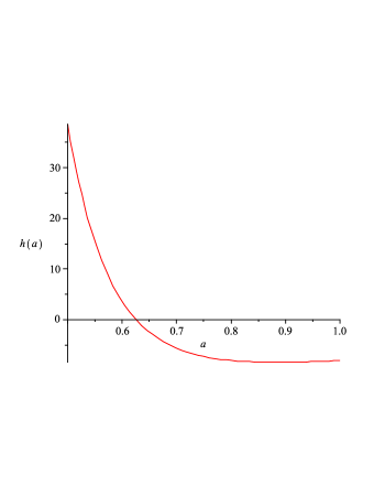
Figure 1: Dust shell occurs at $a_{d}$ where $h(a)$ cuts ${}^{\prime}a^{\prime}$ axis ( choosing suitably the parameters as $M=10$ and $\frac{2\sigma Q^{4}}{5}=.9$ ).

We note that the matter on the junction surface shows peculiar behavior. This matter violates null energy and weak energy conditions but obeys strong energy condition.

Here,

$$\sigma_{s}<0$$ (17)

$$\sigma_{s}+p=-\frac{\left(1-\frac{3M}{a}+\frac{2Q^{2}}{a^{2}}-\frac{3\sigma Q^{4}}{5a^{6}}\right)}{4\pi a\sqrt{1-\frac{2M}{a}+\frac{Q^{2}}{a^{2}}-\frac{\sigma Q^{4}}{5a^{6}}}}<0$$ (18)

$$\sigma_{s}+3p=\frac{\left(1+\frac{M}{a}-\frac{2Q^{2}}{a^{2}}+\frac{7\sigma Q^{4}}{5a^{6}}\right)}{4\pi a\sqrt{1-\frac{2M}{a}+\frac{Q^{2}}{a^{2}}-\frac{\sigma Q^{4}}{5a^{6}}}}>0$$ (19)

Now we measure the Average Null Energy Condition (ANEC) violating matter present in the shell. This can be quantified by the following integrals[19-20]:

$$\Omega_{1}=\int\rho\sqrt{-g}d^{3}x,\Omega_{j}=\int[\rho+p_{j}]\sqrt{-g}d^{3}x$$ (20)

where, $\rho=\sigma_{s}$, the energy condition given in (12) and $p_{j}$, the principal pressures (here, radial pressure $p_{r}$ is zero and transverse pressures $p_{t}=p_{\theta}=p_{\phi}=-v=p=-v_{\theta}=-v_{\phi}$ given in (13)).

Following Eiroa and Simone [11] , we introduce a new radial coordinate $R=\pm(r-a)$ in M ( $\pm$ for $M^{\pm}$ respectively ) so that

$$\Omega_{1}=\int_{0}^{2\pi}\int_{0}^{\pi}\int_{-\infty}^{\infty}\rho\sqrt{-g}dRd{\theta}d{\phi}$$ (21)

$$\Omega_{j}=\int_{0}^{2\pi}\int_{0}^{\pi}\int_{-\infty}^{\infty}[\rho+p_{j}]\sqrt{-g}dRd{\theta}d{\phi}$$ (22)

Since the shell does not exert radial pressure and the energy density is located on a thin shell surface, so that $\rho=\rho+p_{r}=\delta(R)\sigma_{s}$, $\rho+p_{t}=\delta(R)(\sigma_{s}+p_{t})$,

Hence, one gets,

$$\Omega_{r}=\Omega_{1}=\int_{0}^{2\pi}\int_{0}^{\pi}[\sigma_{s}\sqrt{-g}]|_{r=a}d{\theta}d{\phi}=4\pi a^{2}\sigma(a)=-2a\sqrt{1-\frac{2M}{a}+\frac{Q^{2}}{a^{2}}-\frac{\sigma Q^{4}}{5a^{6}}}$$ (23)

$$\Omega_{t}=\int_{0}^{2\pi}\int_{0}^{\pi}[(\sigma_{s}+p_{t})\sqrt{-g}]|_{r=a}d{\theta}d{\phi}=-a\frac{\left(1-\frac{3M}{a}+\frac{2Q^{2}}{a^{2}}-\frac{3\sigma Q^{4}}{5a^{6}}\right)}{\sqrt{1-\frac{2M}{a}+\frac{Q^{2}}{a^{2}}-\frac{\sigma Q^{4}}{5a^{6}}}}$$ (24)

one can see that if the charge of the Reissner-Nordström black hole is kept fixed, then total amount of ANEC violating matter present in the shell is reduced by increasing the mass of the black hole. Obviously this supports our previous analysis ( see eq.(15) ).

4. Stability Analysis:

Rearranging equation (12), we obtain the thin shell’s equation of motion

$$\dot{a}^{2}+V(a)=0$$ (25)

Here the potential is defined as

$$V(a)=1-\frac{2M}{a}+\frac{Q^{2}}{a^{2}}-\frac{\sigma Q^{4}}{5a^{6}}-4\pi^{2}a^{2}\sigma_{s}^{2}(a)$$ (26)

Linearizing around a static solution situated at $a_{0}$, one can expand V(a) around $a_{0}$ to yield

$$V=V(a_{0})+V^{\prime}(a_{0})(a-a_{0})+\frac{1}{2}V^{\prime\prime}(a_{0})(a-a_{0})^{2}+0[(a-a_{0})^{3}]$$ (27)

where prime denotes derivative with respect to $a$.

Since we are linearizing around a static solution at $a=a_{0}$, we have $V(a_{0})=0$ and $V^{\prime}(a_{0})=0$. The stable equilibrium configurations correspond to the condition $V^{\prime\prime}(a_{0})>0$. Now we define a parameter $\beta$, which is interpreted as the speed of sound, by the relation [7]

$$\beta^{2}(\sigma_{s})=\frac{\partial p}{\partial\sigma_{s}}|_{\sigma_{s}}$$ (28)

Here,

$$V^{\prime\prime}(a)=-\frac{4M}{a^{3}}+\frac{6Q^{2}}{a^{4}}-\frac{42\sigma Q^{4}}{5a^{8}}-8\pi^{2}\sigma_{s}^{2}-32\pi^{2}a\sigma_{s}\sigma_{s}^{\prime}-8\pi^{2}a^{2}(\sigma_{s}^{\prime})^{2}-8\pi^{2}a^{2}\sigma_{s}\sigma_{s}^{\prime\prime}$$ (29)

From equations (12) and (13), one can write energy conservation equation as

$$\dot{\sigma_{s}}+2\frac{\dot{a}}{a}(p+\sigma_{s})=0$$ (30)

or

$$\frac{d}{d\tau}(4\pi\sigma_{s}a^{2})+p\frac{d}{d\tau}(4\pi a^{2})=0$$ (31)

From equation (30) ( by using (28) ), we obtain,

$$\sigma_{s}^{\prime\prime}+\frac{2}{a}\sigma_{s}^{\prime}(1+\beta^{2})-\frac{2}{a^{2}}(p+\sigma_{s})=0$$ (32)

The wormhole solution is stable if $V^{\prime\prime}(a_{0})>0$ i.e. if

$$\beta_{0}^{2}<\frac{\left(\frac{3}{2}-\frac{6M}{a_{0}}+\frac{5Q^{2}}{a_{0}^{2}}-\frac{18\sigma Q^{4}}{5a_{0}^{6}}\right)}{1-\frac{2M}{a}+\frac{Q^{2}}{a^{2}}-\frac{\sigma Q^{4}}{5a^{6}}}-\frac{\left(1-\frac{3M}{a_{0}}+\frac{2Q^{2}}{a_{0}^{2}}-\frac{4\sigma Q^{4}}{5a_{0}^{6}}\right)}{2\left(1-\frac{2M}{a}+\frac{Q^{2}}{a^{2}}-\frac{\sigma Q^{4}}{5a^{6}}\right)}-\frac{3}{2}$$ (33)

If one treats $a_{0}$, M , Q and $\sigma$ are specified quantities, then the stability of the configuration requires the above restriction on the parameter $\beta_{0}$. This means there exists some part of the parameter space where the throat location is stable. For a lot of useful information, we show the stability regions graphically ( see figure 2).

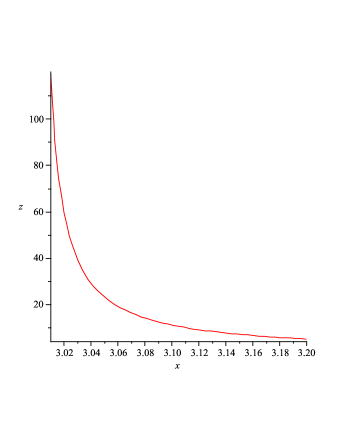
Figure 2: Here we plot $z=\beta^{2}_{|{(a=a_{0})}}$ $Vs.$ $x=\frac{a_{0}}{M}$ ( choosing suitably the parameters as $(\frac{Q}{a_{0}})^{2}=.12$ and $\frac{\sigma Q^{4}}{5a_{0}^{6}}=.1$ ). The stability region is situated below the curve.

5. Discussions:

The minimizing of usage exotic matter needed to construct a wormhole remains an encouraging research area to the scientists working in wormhole physics. Several models and ideas are proposed time to time. Recent observations of gamma ray bursts confirmed that there should exist some sources that produce these bursts. Ruffini and his collaborators argued that these sources are nothing but the dyadospheres. In this work, we have considered a dyadosphere of Reissner-Nordström black hole to develop thin shell wormhole. We have constructed thin shell wormhole by surgically grafting two dyadosphere spacetimes. This study is interesting and more physical since we have used the spacetimes of the astrophysical sources of cosmic gamma ray bursts. We have analyzed the dynamical stability of thin shell wormhole considering linearized radial perturbation around the stable solution. We have shown that there exist some part of the parametric space where the thin shell wormhole is stable. We have also discussed the stability graphically. The most important part of this study is the minimizing of usage of exotic matter confined within the shell. We have seen that Reissner-Nordström black hole mass plays a crucial role to minimize the usage of exotic matter. The Reissner-Nordström black hole with larger mass reduces the amount of exotic matter needed for their construction. Finally, we note that the parameter $\sigma$ coming from the one loop QED in the first order of the approximation is also responsible for reducing the exotic matter.

Acknowledgments

F.R. is thankful to DST , Government of India for providing financial support.

References

- [1] R Ruffini, in XLLX Yamada Conference on Black holes and High Energy Astrophysics, edited by H Salto ( Univ.Acad.Press., Tokyo , 1998 )
- [2] R Ruffini et al, Int.J.Mod.Phys. D 12, 173 (2003)
- [3] R Ruffini, ArXiv: astr-ph/9905072
- [4] G Preparata, R Ruffini and S Xue, Astronmy and Astrophysics L 87, 338 (1998)
- [5] L T Drummond et al, Phys.Rev.D 22, 343 (1980)
- [6] R D Daniels et al, Nucl.Phys.B 425, 635 ( 1994)
- [7] V A De Lorenci et al, Phys.Lett.B 482, 134 (2000)
- [8] M Visser, Nucl.Phys.B 328, 203 ( 1989)
- [9] E Poisson and M Visser, Phys.Rev.D 52, 7318 (1995) [arXiv: gr-qc / 9506083]
- [10] E Eiroa and G Romero, Gen.Rel.Grav. 36, 651 (2004)[arXiv: gr-qc / 0303093]
- [11] E Eiroa and C Simeone, Phys.Rev.D 71, 127501 (2005) [arXiv: gr-qc / 0502073]
- [12] M Thibeault , C Simeone and E Eiroa, arXiv: gr-qc / 0512029
- [13] F.Rahaman , M.Kalam and S.Chakraborty, Gen.Rel.Grav.38:1687-1695,2006. e-Print: gr-qc/0607061
- [14] F.Rahaman , M.Kalam and S.Chakraborti, Int.J.Mod.Phys.D16:1669-1681,2007. e-Print: gr-qc/0611134
- [15] F.Rahaman et al, Gen.Rel.Grav.39:945-956,2007. e-Print: gr-qc/0703143
- [16] F.Rahaman et al, arxiv:0804.3852[gr-qc]
- [17] E Eiroa et al, gr-qc/0404050
- [18] F Lobo, gr-qc/0311002
- [19] M Visser, S Kar and N Dadhich, Phys. Rev.Lett. 90, 201102(2003)[arXiv: gr-qc / 0301003]
- [20] K K Nandi et al , Phys.Rev.D70, 127503(2004)