The analysis of reactions $\pi N\to two\,mesons+N$ within reggeon exchanges.
1. Fit and results.

Abstract

The novel point of this analysis is a direct use of reggeon exchange technique for the description of the reactions $\pi N\to two\,mesons+N$ at large energies of the initial pion. This approach allows us to describe simultaneously distributions over $M$ (invariant mass of two mesons) and $t$ (momentum transfer squared to nucleons). Making use of this technique, the following resonances (as well as corresponding bare states), produced in the $\pi N\to\pi^{0}\pi^{0}N$ reaction are studied: $f_{0}(980)$, $f_{0}(1300)$ ($f_{0}(1370)$ in PDG notation), $f_{0}(1200-1600)$, $f_{0}(1500)$, $f_{0}(1750)$, $f_{2}(1270)$, $f_{2}(1525)$, $f_{2}(1565)$, $f_{2}(2020)$, $f_{4}(2025)$. Adding data for the reactions $p\bar{p}({\rm at\,rest,\,from\,liquid\,H_{2}})\to\pi^{0}\pi^{0}\pi^{0}$, $\pi^{0}\pi^{0}\eta$, $\pi^{0}\eta\eta$ and $p\bar{p}({\rm at\,rest,\,from\,gaseous\,H_{2}})\to\pi^{0}\pi^{0}\pi^{0}$, $\pi^{0}\pi^{0}\eta$, $\pi^{0}\eta\eta$, we have performed simultaneous $K$-matrix fit of two-meson spectra in all these reactions. The results of combined fits to the above-listed isoscalar $f_{J}$-states and to isovector ones, $a_{0}(980)$, $a_{0}(1475)$, $a_{2}(1320)$, are presented.

PACS numbers: 11.25.Hf, 123.1K

1 Introduction

The study of the mass spectrum of hadrons and their properties is the key point for the understanding of colour particle interactions at large distances. But even the meson sector, though less complicated than the baryon one, is far from being completely understood. We mean that
(i) there is no sufficient information about states above 2 GeV,
(ii) certain quark–antiquark states below 2 GeV (e.g. $2^{--}$ states) are still missing,
(iii) there is no clear understanding of the glueball spectrum (although strong candidates in the $0^{++}$ and $2^{++}$ sectors exist, we have no definite information about the $0^{-+}$ sector),
(iv) some analyses reported the observation of other exotics (e.g. hybrid) states,
(v) in the scalar sector not only the properties but also the existence of states like $\sigma$, $\kappa$, $f_{0}(1300)$ ($f_{0}(1370)$ in PDG notation) is under discussion.

So, there is indeed a strong demand for new data which can help us to identify the meson states in a more definite way. However, the situation is only partly connected with the lack of data. In the lower mass region there is a lot of data taken from the proton–antiproton annihilation at rest (Crystal Barrel, Obelix), from the $\gamma\gamma$ interaction (L3), from the proton–proton central collisions (WA102), from $J/\Psi$ decay (Mark III, BES), from $D$- and $B$-meson decays (Focus, D0, BaBar, Belle, Cleo C) and from $\pi N\to two\,mesons+N$ reactions with high energy pion beams (GAMS, VES, E852). Most of these data are of high statistics, thus allowing us to determine resonance properties with a high accuracy (though, let us emphasize, in the reactions $\pi N\to two\,mesons+N$ polarized-target data are lacking).

Nevertheless, in many cases there are significant contradictions between analyses performed by different groups. The ambiguities originate from two circumstances.

First, in the discussed sectors the analyses of data taken from a single experiment cannot provide us with a unique solution. A unique solution can be obtained only from the combined analysis of a large set of data taken in different experiments.

Second, there are some simplifications inherent in many analyses. The unitarity was neglected frequently even when the amplitudes were close to the unitarity limit. A striking example is that up to now there is no proper $K$-matrix parametrization of the $1^{--}$ and $2^{++}$ waves which are considered by many physicists as mostly understood ones. As to multipartical final states, only a few analyses have ever considered the contributions of triangle or box singularities to the measured cross sections. However, these contributions can simulate the resonant behavior of the studied distributions, especially in the threshold region (for more detail, see [1] and references therein).

In the analysis of meson spectra in high energy reactions $\pi N\to two\,mesons+N$, many results are related to the decomposition of the cross sections into natural and unnatural amplitudes that is based on certain models developed for the two-pion production at small momenta transferred, (e.g., see [2, 3, 4]). However, as was discussed by the cited authors, a direct application of these methods at large momenta transferred to the analysis of data may lead to a wrong result. In addition, the $\pi N\to two\,mesons+N$ data were discussed mostly in terms of $t$-channel particle exchange, though without proper analysis of the $t$-channel exchange amplitudes.

A decade ago our group performed a combined analysis of data on proton–antiproton annihilation at rest into three pseudoscalar mesons, together with the data on two-meson $S$-waves extracted form the $\pi N\to\pi\pi N$, $\eta\eta N$, $K\bar{K}$ and $\eta\eta^{\prime}N$ reactions [5, 6, 7]. The analysis has been carried out in the framework of the $K$-matrix approach which preserves unitarity and analyticity of the amplitude in the two-meson physical region. Although the two-meson data extracted from the reaction $\pi N\to two\,mesons+N$ at small momentum transfer appeared to be highly compatible with those found in proton–antiproton annihilation, we have faced a set of problems, describing the $\pi N\to two\,mesons+N$ data at large momentum transfer. As we have seen now, the problems were owing to the use of partial wave decomposition which was performed by the E852 Collaboration and showed a huge signal at 1300 MeV in the $S$-wave.

The strategy of our present approach is as follows. The analysis of a large set of experimental data on proton–antiproton annihilation at rest is carried out together with the analysis of the $\pi N\to two\,mesons+N$ data based on the $t$-channel reggeized exchanges. For the $\pi N\to two\,mesons+N$ reactions, the data at small and large momentum transfers are included. Here, as the first step, we perform the analysis in the framework of the $K$-matrix parametrization for all fitting channels ($K$-matrix approach insures the unitarity and analyticity in the physical region). At the next stage, we plan to use the $N/D$ method for two-meson amplitudes satisfying these requirements in the whole complex plane.

In this paper, we present the method for the analysis of the $\pi N$ interactions based on the $t$-channel reggeized exchanges supplemented by a study of the proton–antiproton annihilation at rest. The method is applied to a combined analysis of the $\pi N\to\pi^{0}\pi^{0}N$ data taken by E852 at small and large momentum transfers and Crystal Barrel data on the proton–antiproton annihilation at rest into three neutral pseudoscalar mesons. The even waves, which contributed to this set of data, are parametrized within the $K$-matrix approach. To check a strong $S$-wave signal around 1300 MeV, which has been reported by E852 Collaboration from the analysis of data at large momentum transfers, is a subject of a particular interest in the present analysis.

We present the results of the new $K$-matrix analysis of two-meson spectra in the scalar, $J^{P}=0^{+}$, and tensor, $J^{P}=2^{+}$, sectors: these sectors need a particular attention because just here we meet with the low-lying glueballs, $f_{0}(1200-1600)$ and $f_{2}(2000)$. The situation with the tensor glueball is rather transparent allowing us to make a definite conclusion about the gluonium structure of $f_{2}(2000)$, while the status of the broad state $f_{0}(1200-1600)$ requires a special discussion: this state is nearly flavour-blind but the corresponding pole of the amplitude dives deeply into the complex-$M$ plane. It is definitely seen only in the analysis of a large number of different reactions in broad intervals of mass spectra (for example, see [1] and references therein).

So, here we consider the following reactions:
(i) $\pi p\to\pi^{0}\pi^{0}n$ at high energies of initial pion and small and large momenta transferred to nucleon, and
(ii) $p\bar{p}({\rm at\,rest\,H_{2}})\to\pi^{0}\pi^{0}\pi^{0}$, $\pi^{0}\pi^{0}\eta$, $\pi^{0}\eta\eta$ in liquid and gaseous $H_{2}$ — the data on these reactions give us the most reliable information about scalar and tensor sectors.
As was stressed above, the novel point of the performed $K$-matrix analysis is the use of reggeon exchange technique for the description of $\pi p\to\pi\pi n$ at high energies that allows us to analyze the two-meson invariant mass spectra and nucleon momentum transfer distributions simultaneously.

The paper is organized as follows.

In Section 2, we consider meson–nucleon collisions at high energies and present formulas for peripheral two-meson production amplitudes in terms of reggeon exchanges. Amplitudes for the description of low-energy three-meson production in the $K$-matrix approach are given in Section 3. The fitting procedure is described in Section 4. In Conclusion we summarize the results. Technical aspects of the fitting procedure are discussed in [8].

2 Meson–Nucleon Collisions at High Energies: Peripheral Two-Meson Production in Terms of Reggeon Exchanges

The two-meson production reactions $\pi p\to\pi\pi n$, $K\bar{K}n$, $\eta\eta n$, $\eta\eta^{\prime}n$ at high energies and small momentum transfers to the nucleon are used for obtaining the $S$-wave amplitudes $\pi\pi\to\pi\pi$, $K\bar{K}$, $\eta\eta$, $\eta\eta^{\prime}$ at $|t|<0.2\,(\rm GeV/c)^{2}$ because, as commonly believed, the $\pi$ exchange dominates this wave at such momentum transferred. At larger momentum transfers, $|t|\mathrel{\mathchoice{\lower 3.6pt\vbox{\halign{$\mathsurround=0pt\displaystyle\hfil#\hfil$\cr>\crcr\sim\crcr}}}{\lower 3.6pt\vbox{\halign{$\mathsurround=0pt\textstyle\hfil#\hfil$\cr>\crcr\sim\crcr}}}{\lower 3.6pt\vbox{\halign{$\mathsurround=0pt\scriptstyle\hfil#\hfil$\cr>\crcr\sim\crcr}}}{\lower 3.6pt\vbox{\halign{$\mathsurround=0pt\scriptscriptstyle\hfil#\hfil$\cr>\crcr\sim\crcr}}}}0.2\,(\rm GeV/c)^{2}$, we observe definitely a change of the regime in the $S$-wave production — a significant contribution of other reggeons is possible ($a_{1}$-exchange, daughter-$\pi$ and daughter-$a_{1}$ exchanges). Nevertheless, the study of the two-meson production processes at $|t|\sim 0.5-1.5\,(\rm GeV/c)^{2}$ looks promising, for at such momentum transfers the contribution of the broad resonance (the scalar glueball $f_{0}(1200-1600)$) vanishes. Therefore, the production of other resonances (such as the $f_{0}(980)$ and $f_{0}(1300)$) appears practically without background – this is important for finding out their characteristics as well as a mechanism of their production.

What we know about the reactions $\pi p\to\pi\pi n$, $K\bar{K}n$, $\eta\eta n$, $\eta\eta^{\prime}n$ allows us to suggest that a consistent analysis of the peripheral two-meson production in terms of reggeon exchanges may be a good tool for studying meson resonances. Note that investigation of two-meson scattering amplitudes by means of the reggeon exchange expansion of the peripheral two-meson production amplitudes was proposed long ago [9] but was not used because of the lack of data until now.

The $K$-matrix amplitude of the peripheral production of two mesons with total angular momentum $J$ reads:

$$\bigg{(}\bar{\psi}_{N}(k_{3})\hat{G}_{R}\psi_{N}(p_{2})\bigg{)}R(s_{\pi N},t)\widehat{K}_{\pi R(t)}(s)\bigg{[}1-\hat{\rho}(s)\widehat{K}(s)\bigg{]}^{-1}Q^{(J)}(k_{1},k_{2})\ ,$$ (1)

This formula is illustrated by Fig. 1 for the production of $\pi\pi$, $K\bar{K}$, $\eta\eta$, $\eta\eta^{\prime}$ systems. Here the factor $(\bar{\psi}_{N}(k_{3})\hat{G}_{R}\psi_{N}(p_{2}))$ stands for the reggeon–nucleon vertex, and $\hat{G}_{R}$ is the spin operator; $R(s_{\pi N},t)$ is the reggeon propagator depending on the total energy squared of colliding particles, $s_{\pi N}=(p_{1}+p_{2})^{2}$, and the momentum transfer squared $t=(p_{2}-k_{3})^{2}$, while the factor $\widehat{K}_{\pi R(t)}[1-i\hat{\rho}(s)\widehat{K}(s)]^{-1}$ is related to the block of two-meson production; $s\equiv M^{2}=(k_{1}+k_{2})^{2}$, and $\hat{\rho}(s)$ is the phase space matrix . In the reactions $\pi p\to\pi\pi n$, $K\bar{K}n$, $\eta\eta n$, $\eta\eta^{\prime}n$, the factor $\widehat{K}_{\pi R(t)}(s)[1-i\hat{\rho}(s)\widehat{K}(s)]^{-1}$ describes transitions $\pi R(t)\to\pi\pi$, $K\bar{K}$, $\eta\eta$, $\eta\eta^{\prime}$: in this way the block $\widehat{K}_{\pi R(t)}$ is associated with the prompt meson production, and $[1-i\hat{\rho}(s)\widehat{K}(s)]^{-1}$ is the $K$-matrix factor for meson rescattering (of the type of $\pi\pi\to\pi\pi$, $\pi\pi\to K\bar{K}$, $K\bar{K}\to\eta\eta$, and so on). The prompt-production block for transition $\pi R\to b$ (where $b=\pi\pi$, $K\bar{K}$, $\eta\eta$, $\eta\eta^{\prime}$, $4\pi$, …) is parameterized with singular (pole) and smooth terms [5, 7, 10]:

$$\left(\widehat{K}_{\pi R(t)}\right)_{\pi R,b}\ =\ \sum_{n}\frac{G^{(n)}_{\pi R}(t)g^{(n)}_{b}}{\mu^{2}_{n}-s}+f_{\pi R,b}(t,s)\ .$$ (2)

The pole singular term, $G^{(n)}_{\pi R}(t)g^{(n)}_{b}/(\mu^{2}_{n}-s)$, determines the bare state: here $G^{(n)}_{\pi R}(t)$ is the bare state production vertex while the parameters $g^{(n)}_{b}$ and $\mu_{n}$ are the coupling and the mass of the bare state – they are the same as in the partial wave transition amplitudes $\pi\pi\to\pi\pi$, $K\bar{K}$, $\eta\eta$, $\eta\eta^{\prime}$, $4\pi$, $...$. The smooth term $f_{\pi R,b}$ stands for the background production of mesons. The $G^{(n)}_{\pi R}(t)$, $f_{\pi R,b}$, $g^{(n)}_{b}$, $\mu_{n}$ are free parameters of the fitting procedure, while the characteristics of resonances are determined by poles of the $K$-matrix amplitude (remind that the position of poles is given by zeros of the amplitude denominator, $det|1-\hat{\rho}(s)\widehat{K}(s)|=0$).

Figure 1: Example of a reaction with the production of two mesons (here $\pi\pi$, $K\bar{K}$, $\eta\eta$, $\eta\eta^{\prime}$ in $\pi^{-}p$ collision) due to reggeon ($R$) exchange.

Below we explain in detail the method of analysis of meson spectra using as an example the reactions $\pi N\to\pi\pi N$, $K\bar{K}N$, $\eta\eta N$, $\eta\eta^{\prime}N$, $\pi\pi\pi\pi N$.

2.1 Reggeon exchange technique and the $K$-matrix analysis of meson spectra in the waves $J^{PC}=0^{++}$, $1^{--}$, $2^{++}$, $3^{--}$, $4^{++}$ in high energy reactions $\pi N\to two\;mesons+N$

Here we present the technique of the analysis of high-energy reaction $\pi^{-}p\to mesons+n$, with the production of mesons in the $J^{PC}=0^{++}$, $1^{--}$, $2^{++}$, $3^{--}$, $4^{++}$ states at small and moderate momenta transferred to the nucleon.

The following points are to be emphasized:
(1) The technique can be used for performing the $K$-matrix analysis not only for $0^{++}$ and $2^{++}$ wave, as in [5, 7, 10], but simultaneously in $1^{--}$, $3^{--}$, $4^{++}$ waves as well.
(2) We use the reggeon exchange technique for the description of the $t$-dependence in all analyzed amplitudes. This allows us to perform a partial wave decomposition of the produced meson states directly on the basis of the measured cross sections without using the published moment expansions (which were done under some simplifying assumptions – it is discussed below in more detail).
(3) The mass interval of the analyzed spectra is extended up to 2500 MeV thus overlapping with the mass region studied in reactions $p\bar{p}$(in flight)$\to\,mesons$ [11].

We discuss in detail the reactions at incident pion momenta 20–50 GeV/c, such as measured in [12, 13, 14, 15, 16, 17]: (i) $\pi^{-}p\to\pi^{+}\pi^{-}+n$, (ii) $\pi^{-}p\to\pi^{0}\pi^{0}+n$, (iii) $\pi^{-}p\to K_{S}K_{S}+n$, (iv) $\pi^{-}p\to\eta\eta+n$. At these energies, the mesons in the states $J^{PC}=0^{++}$, $1^{--}$, $2^{++}$, $3^{--}$, $4^{++}$ are produced via $t$-channel exchange by reggeized mesons belonging to the leading and daughter $\pi$, $a_{1}$ and $\rho$ trajectories.

But, first, let us present notations used below.

2.1.1 Cross sections for the reactions ${\pi}N\to\pi\pi N$, $KKN$, $\eta\eta N$

We consider the process of the Fig. 1 type, that is, $\pi N$ interaction at large momenta of the incoming pion with the production of a two-meson system with a large momentum in the beam direction. This is a peripheral production of two mesons.

The cross section is defined as follows:

$$d\sigma=\frac{(2\pi)^{4}|A|^{2}}{8\sqrt{s_{{\pi}N}}|\vec{p}_{2}|_{cm(\pi p)}}\,d\phi(p_{1}+p_{2};k_{1},k_{2},k_{3}),$$

$$d\phi(p_{1}+p_{2};k_{1},k_{2},k_{3})=(2\pi)^{3}d\Phi(P;k_{1},k_{2})\,d\Phi(p_{1}+p_{2};P,k_{3})\,ds\,,$$ (3)

where $|\vec{p_{2}}|_{cm(\pi p)}$ is the pion momentum in the c.m. frame of the incoming hadrons. Taking into account that invariant variables $s$ and $t$ are inherent in the meson peripheral amplitude, we rewrite the phase space in a more convenient form:

$$d\Phi(p_{1}+p_{2};P,k_{3})=\frac{1}{(2\pi)^{5}}\frac{dt}{8|\vec{p_{2}}|_{cm(\pi p)}\sqrt{s_{{\pi}N}}},\qquad t=(k_{3}-p_{2})^{2},$$

$$d\Phi(P;k_{1},k_{2})=\frac{1}{(2\pi)^{5}}\rho(s)d\Omega\,,\qquad\rho(s)=\frac{1}{16\pi}\frac{2|\vec{k}_{1}|_{cm(12)}}{\sqrt{s}}.$$ (4)

Momentum $|\vec{k}_{1}|_{cm(12)}$ is calculated in the c.m. frame of the outgoing mesons: in this system one has $P=(M,0,0,0,)\equiv(\sqrt{s},0,0,0)$ and $g_{\mu\nu}^{\perp P}k_{1\nu}=-g_{\mu\nu}^{\perp P}k_{2\nu}=(0,k\,\sin\Theta\sin\varphi,\,k\,\cos\Theta\sin\varphi$, $k\,\cos\Theta\,k)$ while $d\Omega=d(\cos\Theta)d\varphi$. We have:

$$d\sigma=\frac{(2\pi)^{4}|A|^{2}(2\pi)^{3}}{8|\vec{p_{2}}|_{cm(\pi p)}\sqrt{s_{{\pi}N}}}\frac{1}{(2\pi)^{5}}\frac{dt\,dM^{2}\,d\Phi(P,k_{1},k_{2})}{8|\vec{p}_{2}|_{cm(\pi p)}\sqrt{s_{\pi N}}}=\frac{|A|^{2}\rho(M^{2})\,MdM\,dt\,d\Omega}{32(2\pi)^{3}|\vec{p}_{2}|^{2}_{cm(\pi p)}\,s_{\pi N}}.~{}~{}$$ (5)

The cross section can be expressed in terms of the spherical functions:

$$\frac{d^{4}\sigma}{dt{d\Omega}dM}=N(M,t)\sum\limits_{l}\bigg{(}{\langle{Y}^{0}_{l}\rangle}Y^{0}_{l}(\Theta,\varphi)+2\sum\limits_{m=1}^{l}{\langle{Y}^{m}_{l}\rangle}{\rm Re}\,Y^{m}_{l}(\Theta,\varphi)\bigg{)}.$$ (6)

The coefficients $N(M,t)$, $\langle{Y}^{0}_{l}\rangle$, $\langle{Y}^{m}_{l}\rangle$ are subjects of study in the determination of meson resonances.

Before describing the results of analysis based on the reggeon exchange technique, let us comment methods used in other approaches.

2.1.2 The CERN-Munich approach

The CERN-Munich model [15] was developed for the analysis of the data on the $\pi^{-}p\to\pi^{+}\pi^{-}n$ reaction. It is based partly on the absorption model but mainly on phenomenological observations. The amplitude squared is written as

$$|A|^{2}=\bigg{|}\sum\limits_{J=0}A^{0}_{J}Y^{0}_{J}(\Theta,\varphi)+\sum\limits_{J=1}A^{(-)}_{J}ReY^{1}_{J}(\Theta,\varphi)\bigg{|}^{2}+\bigg{|}\sum\limits_{J=1}A^{(+)}_{J}ReY^{1}_{J}(\Theta,\varphi)\bigg{|}^{2}\ ,$$ (7)

and additional assumptions are made:
1) The helicity-1 amplitudes are equal for natural and unnatural exchanges $A^{(-)}_{J}=A^{(+)}_{J}$;
2) The ratio of the $A^{(-)}_{J}$ and the $A^{0}_{J}$ amplitudes is a polynomial over the mass of the two-pion system which does not depend on $J$ up to the total normalization, $A^{(-)}_{J}=A^{0}_{J}\bigg{(}C_{J}\sum\limits^{3}_{n=0}b_{n}M^{n}\bigg{)}^{-1}$.
Then, in [15], the amplitude squared was rewritten using density matrices $\rho^{nm}_{00}=A^{0}_{n}A^{0*}_{m}$, $\rho^{nm}_{01}=A^{0}_{n}A^{(-)*}_{m}$, $\rho^{nm}_{11}=2A^{(-)}_{n}A^{(-)}_{m}$ as follows:

$$|A|^{2} = \sum\limits_{J=0}Y^{0}_{J}(\Theta,\varphi)\left(\sum\limits_{n,m}d^{0,0,0}_{n,m,J}\rho^{nm}_{00}+d^{1,1,0}_{n,m,J}\rho^{nm}_{11}\right)$$

$$+ \sum\limits_{J=0}ReY^{1}_{J}(\Theta,\varphi)\left(\sum\limits_{n,m}d^{1,0,1}_{n,m,J}\rho^{nm}_{10}+d^{0,1,1}_{n,m,J}\rho^{mn}_{11}\right),$$

$$d^{i,k,l}_{n,m,J} = \frac{\int d\Omega\,ReY^{i}_{n}(\Theta,\varphi)\,ReY^{k}_{m}(\Theta,\varphi)\,ReY^{l}_{J}(\Theta,\varphi)}{\int d\Omega\,ReY^{l}_{J}(\Theta,\varphi)\,ReY^{l}_{J}(\Theta,\varphi)}.$$ (8)

Using this amplitude for the cross section, the fitting to the moments $<Y^{m}_{J}>$ has been carried out.

The CERN–Munich approach cannot be applied to large $t$, it does not work for many other final states either.

2.1.3 GAMS, VES, and BNL approaches

In GAMS [12, 13], VES [16], and BNL [17] approaches, the $\pi N$ data are described by a sum of amplitudes squared with an angular dependence defined by spherical functions:

$$|A^{2}|\!=\!\bigg{|}\sum\limits_{J=0}A^{0}_{J}Y^{0}_{J}(\Theta,\varphi)\!+\!\sum\limits_{J=1}A^{(-)}_{J}\sqrt{2}\,Re\,Y^{1}_{J}(\Theta,\varphi)\bigg{|}^{2}\!\!+\!\bigg{|}\sum\limits_{J=1}A^{(+)}_{J}\sqrt{2}\,Im\,Y^{1}_{J}(\Theta,\varphi)\bigg{|}^{2}~{}~{}$$ (9)

The $A^{0}_{J}$ functions are denoted as $S_{0},P_{0},D_{0},F_{0}\ldots$, the $A^{(-)}_{J}$ functions are defined as $P_{-},D_{-},F_{-},\ldots$ and the $A^{(+)}_{J}$ functions as $P_{+},D_{+},F_{+},\ldots$. The equality of the helicity-1 amplitudes with natural and unnatural exchanges is not assumed in these approaches.

However, the discussed approaches are not free from other assumptions like the coherence of some amplitudes or the dominance of the one-pion exchange. In reality the interference of the amplitudes being determined by $t$-channel exchanges of different particles leads to a more complicated picture than that given by (9), this latter may lead (especially at large $t$) to a misidentification of quantum numbers for the produced resonances.

For example, in [17] the S-wave appears in an unnatural set of amplitudes only. Natural exchanges have moments with m=1,2,3…. However, the a1-exchange is a natural one, therefore it contributes into the S-wave and does not interfere with unnatural exchanges – in this point the moment expansion [17] does not coincide with formula with reggeon exchanges.

2.2 The $t$-channel exchanges of pion trajectories in the reaction $\pi^{-}p\to\pi\pi\,n$

Consider now in more detail the production amplitude for the $\pi\pi$ system with $I=0$ and $J^{PC}=0^{++},2^{++}$ and show the way of its generalization for higher $J$.

2.2.1 Amplitude with leading and daughter pion trajectory exchanges

The amplitude with $t$-channel pion trajectory exchanges can be written as follows:

$$A_{\pi p\to\pi\pi n}^{(\pi-{\rm trajectories})}\!=\!\sum\limits_{R(\pi_{j})}\!A\bigg{(}\pi R(\pi_{j})\to\pi\pi\bigg{)}R_{\pi_{j}}(s_{\pi N},q^{2})\left(\varphi_{n}^{+}(\vec{\sigma}\vec{q}_{\perp})\varphi_{p}\right)g^{(\pi_{j})}_{pn}(t)~{}~{}~{}$$ (10)

The summation is carried out over the leading and daughter trajectories. Here $A(\pi R(\pi_{j})\to\pi\pi)$ is the transition amplitude for meson block in Fig. 1, $g^{(\pi_{j})}_{pn}$ is the reggeon–$NN$ coupling and $R_{\pi_{j}}(s_{\pi N},q^{2})$ is the reggeon propagator:

$$R_{\pi_{j}}(s_{\pi N},q^{2})\!=\!\exp{\left(\!-i\frac{\pi}{2}\alpha^{(j)}_{\pi}(q^{2})\!\right)}\frac{\left(s_{\pi N}/s_{\pi N0}\right)^{\alpha^{(j)}_{\pi}(q^{2})}}{\sin\left(\frac{\pi}{2}\alpha^{(j)}_{\pi}(q^{2})\right)\Gamma\left(\frac{1}{2}\alpha^{(j)}_{\pi}(q^{2})+1\right)}.$$ (11)

The $\pi$–reggeon has a positive signature, $\xi_{\pi}=+1$. Following [1, 18, 19, 20], we use for pion trajectories:

$$\alpha_{\pi}^{(leading)}(q^{2})\simeq-0.015+0.72q^{2},\quad\alpha_{\pi}^{(daughter-1)}(q^{2})\simeq-1.10+0.72q^{2},~{}~{}~{}$$ (12)

where the slope parameters are given in (GeV/c)^-2 units. The normalization parameter $s_{\pi N0}$ is of the order of 2–20 GeV². To eliminate the poles at $q^{2}<0$ we introduce Gamma-functions in the reggeon propagators (recall that $1/\Gamma(x)=0$ at $x=0,-1,-2,\ldots$).

For the nucleon–reggeon vertex $\hat{G}^{(\pi)}_{pn}$ we use in the infinite momentum frame the two-component spinors $\varphi_{p}$ and $\varphi_{n}$ (see, for example, [1, 18, 21]):

$$g_{\pi}(\bar{\psi}(k_{3})\gamma_{5}\psi(p_{2}))\longrightarrow\left(\varphi_{n}^{+}(\vec{\sigma}\vec{q}_{\perp})\varphi_{p}\right)g^{(\pi)}_{pn}(t)\,.$$ (13)

As to the meson–reggeon vertex, we use the covariant representation [1, 18, 22]. For the production of two pseudoscalar particles (let it be $\pi\pi$ in the considered case), it reads:

$$A\bigg{(}\pi R(\pi_{j})\to\pi\pi\bigg{)}\!=\!\sum\limits_{J}A^{(J)}_{\pi R(\pi_{j})\to\pi\pi}(s)X^{(J)}_{\mu_{1}\ldots\mu_{J}}(p^{\perp})\,(-1)^{J}O^{\mu_{1}\ldots\mu_{J}}_{\nu_{1}\ldots\nu_{J}}(\perp P)X^{(J)}_{\nu_{1}\ldots\nu_{J}}(k^{\perp})\,\xi_{J}\,,$$

$$\xi_{J}=\frac{16\pi(2J+1)}{\alpha_{J}},\qquad\alpha_{J}=\prod\limits^{J}_{n=1}\frac{2n-1}{n}.~{}~{}~{}~{}~{}~{}~{}~{}~{}~{}~{}~{}~{}~{}~{}~{}~{}~{}~{}~{}~{}~{}~{}~{}~{}~{}~{}~{}~{}~{}~{}~{}~{}~{}~{}$$ (14)

The angular momentum operators are constructed of momenta $p^{\perp}$ and $k^{\perp}$ which are orthogonal to the momentum of the two-pion system $P=k_{1}+k_{2}$:

$$g_{\mu\nu}^{\perp}=g_{\mu\nu}-\frac{P_{\mu}P_{\nu}}{P^{2}},\qquad k^{\perp}_{\mu}=\frac{1}{2}(k_{1}-k_{2})_{\nu}g^{\perp}_{\mu\nu}\qquad p^{\perp}_{\mu}=\frac{1}{2}(p_{1}+q)_{\nu}g^{\perp}_{\mu\nu}\,.$$ (15)

The coefficient $\xi_{J}$ normalizes the angular momentum operators, so that the unitarity condition appears in a simple form (for details see Appendix A).

2.2.2 The $t$-channel $\pi_{2}$-exchange

The $R(\pi_{j})$-exchanges dominate the spin flip amplitudes, and the amplitudes with $m=1$ are here suppressed, see (6). However, their contributions are visible in the differential cross sections and should be taken into account. The effects appear owing to the interference in the two-meson production amplitude because of the reggeized $\pi_{2}$ exchange in the $t$-channel. The corresponding amplitude is written as:

$$\sum\limits_{a}A_{\alpha\beta}\bigg{(}\pi R(\pi_{2})\to\pi\pi\bigg{)}\varepsilon^{(a)}_{\alpha\beta}R_{\pi_{2}}(s_{\pi N},q^{2})\frac{\varepsilon^{(a)+}_{\alpha^{\prime}\beta^{\prime}}}{s^{2}_{\pi N}}X^{(2)}_{\alpha^{\prime}\beta^{\prime}}(k_{3}^{\perp q})\left(\varphi_{n}^{+}(\vec{\sigma}\vec{q}_{\perp})\varphi_{p}\right)g^{(\pi_{2})}_{pn}(t)\ ,$$ (16)

where $A_{\alpha\beta}\bigg{(}\pi R(\pi_{2})\to\pi\pi\bigg{)}$ is the meson block of the amplitude related to the $\pi_{2}$-reggeized $t$-channel transition, $g^{(\pi_{2})}_{pn}$ is the reggeon–$pn$ vertex, $R_{\pi_{2}}(s_{\pi N},q^{2})$ is the reggeon propagator, and $\varepsilon^{(a)}_{\alpha\beta}$ is the polarization tensor for the $2^{-+}$ state. Let us remind that $k_{3}$ is the momentum of the outgoing nucleon.

$$k_{3\mu}^{\perp q}=g^{\perp q}_{\mu\nu}k_{3\nu}\qquad g^{\perp q}_{\mu\nu}=g_{\mu\nu}-\frac{q_{\mu}q_{\nu}}{q^{2}}\,.$$ (17)

The $\pi_{2}$ particles are located on the pion trajectories and are described by a similar reggeized propagator. But in the meson block, the $2^{-+}$ state exchange leads to vertices different from those in the $0^{-+}$-exchange, so it is convenient to single out these contributions. Therefore, we use for $R_{\pi_{2}}(s_{\pi N},q^{2})$ the propagator given by (11) but with eliminated $\pi(0^{-+})$-contribution:

$$R_{\pi_{2}}(s_{\pi N},q^{2})=\exp{\left(-i\frac{\pi}{2}\alpha^{(leading)}_{\pi}(q^{2})\right)}\frac{\left(s_{\pi N}/s_{\pi N0}\right)^{\alpha^{(leading)}_{\pi}(q^{2})}}{\sin\left(\frac{\pi}{2}\alpha^{(leading)}_{\pi}(q^{2})\right)\Gamma\left(\frac{1}{2}\alpha^{(leading)}_{\pi}(q^{2})\right)}\,.$$ (18)

Taking into account that

$$\sum\limits_{a=1}^{5}\varepsilon^{(a)}_{\alpha\beta}\varepsilon^{(a)+}_{\alpha^{\prime}\beta^{\prime}}=\frac{1}{2}\left(g^{\perp q}_{\alpha\alpha^{\prime}}g^{\perp q}_{\beta\beta^{\prime}}+g^{\perp q}_{\beta\alpha^{\prime}}g^{\perp q}_{\alpha\beta^{\prime}}-\frac{2}{3}g^{\perp q}_{\alpha\beta}g^{\perp q}_{\alpha^{\prime}\beta^{\prime}}\right)\,,$$ (19)

one obtains:

$$\frac{X^{(2)}_{\alpha^{\prime}\beta^{\prime}}(k_{3}^{\perp q})}{2s^{2}_{\pi N}}\left(g^{\perp q}_{\alpha\alpha^{\prime}}g^{\perp q}_{\beta\beta^{\prime}}+g^{\perp q}_{\beta\alpha^{\prime}}g^{\perp q}_{\alpha\beta^{\prime}}-\frac{2}{3}g^{\perp q}_{\alpha\beta}g^{\perp q}_{\alpha^{\prime}\beta^{\prime}}\right)=\frac{3}{2}\frac{k^{\perp q}_{3\alpha}k^{\perp q}_{3\beta}}{s^{2}_{\pi N}}-\frac{4m_{N}^{2}-q^{2}}{8s^{2}_{\pi N}}\left(g_{\alpha\beta}-\frac{q_{\alpha}q_{\beta}}{q^{2}}\right)\ .$$ (20)

In the large momentum limit of the initial pion, the second term in (20) is always small and can be neglected, while the convolution of $k^{\perp q}_{3\alpha}k^{\perp q}_{3\beta}$ with the momenta of the meson block results in the term $\sim s^{2}_{\pi N}$. Hence, the amplitude for $\pi_{2}$-exchange can be rewritten as follows:

$$A_{\pi p\to\pi\pi n}^{(\pi_{2}-{\rm exchange})}=\frac{3}{2}A_{\alpha\beta}(\pi R(\pi_{2})\to\pi\pi)\frac{k^{\perp q}_{3\alpha}k^{\perp q}_{3\beta}}{s^{2}_{\pi N}}R_{\pi_{2}}(s_{\pi N},q^{2})\left(\varphi_{n}^{+}(\vec{\sigma}\vec{q}_{\perp})\varphi_{p}\right)g^{(\pi_{2})}_{pn}\,.$$ (21)

A resonance with spin $J$ and fixed parity can be produced owing to the $\pi_{2}$-exchange with three angular momenta $L=J-2$, $L=J$ and $L=J+2$, so we have:

$$A_{\alpha\beta}(\pi R(\pi_{2})\to\pi\pi)=\sum\limits_{J}A^{(J)}_{+2}(s)X^{(J+2)}_{\alpha\beta\mu_{1}\ldots\mu_{J}}(p^{\perp})(-1)^{J}O^{\mu_{1}\ldots\mu_{J}}_{\nu_{1}\ldots\nu_{J}}(\perp P)X^{(J)}_{\nu_{1}\ldots\nu_{J}}(k^{\perp})\xi_{J}$$

$$+\sum\limits_{J}A^{(J)}_{0}(s)O_{\chi\tau}^{\alpha\beta}(\perp q)X^{(J)}_{\chi\mu_{2}\ldots\mu_{J}}(p^{\perp})(-1)^{J}O^{\tau\mu_{2}\ldots\mu_{J}}_{\nu_{1}\nu_{2}\ldots\nu_{J}}(\perp P)X^{(J)}_{\nu_{1}\ldots\nu_{J}}(k^{\perp})\xi_{J}$$

$$+\sum\limits_{J}A^{(J)}_{-2}(s)X^{(J-2)}_{\mu_{3}\ldots\mu_{J}}(p^{\perp})(-1)^{J}O^{\alpha\beta\mu_{3}\ldots\mu_{J}}_{\nu_{1}\nu_{2}\nu_{3}\ldots\nu_{J}}(\perp P)X^{(J)}_{\nu_{1}\ldots\nu_{J}}(k^{\perp})\xi_{J}\ .$$ (22)

The sum of the two terms presented in (10) and (21) gives us an amplitude with a full set of the $\pi_{j}$-meson exchanges.

Let us emphasize an important point: in the $K$-matrix representation the amplitudes $A^{(J)}_{\pi R(\pi_{j})\to\pi\pi}(s)$ (Eq. (2.2.1), $j=leading,daughter$-1) and $A^{(J)}_{+2}(s)$, $A^{(J)}_{0}(s)$, $A^{(J)}_{-2}(s)$ (Eq. (22)) differ only due to the prompt-production $K$-matrix block (the term $\widehat{K}_{\pi R(t)}(s)$ in (1)) while the final state interaction factor ($[1-\hat{\rho}(s)\widehat{K}(s)]^{-1}$ in (1)) is the same for each $J$.

2.3 Amplitudes with $a_{J}$-trajectory exchanges

Here we present formulae for for leading and daughter $a_{1}$-trajectories and leading $a_{2}$-trajectory.

2.3.1 Amplitudes with $a_{1}$-trajectory exchanges

The amplitude with $t$-channel $a_{1}$-exchanges is a sum of leading and daughter trajectories:

$$A_{\pi p\to\pi\pi n}^{(a_{1}{\rm-trajectories})}=\sum\limits_{a_{1}^{(j)}}A\left(\pi R(a_{1}^{(j)})\to\pi\pi\right)R_{a^{(j)}_{1}}(s_{\pi N},q^{2})i\left(\varphi_{n}^{+}(\vec{\sigma}\vec{n}_{z})\varphi_{p}\right)g^{(a_{1j})}_{pn}(t)\ ,$$ (23)

where $g^{(a_{1j})}_{pn}$ is the reggeon–NN coupling and the reggeon propagator $R_{a_{1}^{(j)}}(s_{\pi N},q^{2})$ has the form:

$$R_{a_{1}^{(j)}}(s_{\pi N},q^{2})=i\exp{\left(-i\frac{\pi}{2}\alpha^{(j)}_{a_{1}}(q^{2})\right)}\frac{\left(s_{\pi N}/s_{\pi N0}\right)^{\alpha^{(j)}_{a_{1}}(q^{2})}}{\cos\left(\frac{\pi}{2}\alpha^{(j)}_{a_{1}}(q^{2})\right)\Gamma\left(\frac{1}{2}\alpha^{(j)}_{a_{1}}(q^{2})+\frac{1}{2}\right)}\,.$$

Recall that the $a_{1}$ trajectories have a negative signature, $\xi_{\pi}=-1$. Here we take into account the leading and first daughter trajectories which are linear and have a universal slope parameter [18, 19, 20]:

$$\alpha_{a_{1}}^{(leading)}(q^{2})\simeq-0.10+0.72q^{2},\quad\alpha_{a_{1}}^{(daughter-1)}(q^{2})\simeq-1.10+0.72q^{2}.$$ (25)

As previously, the normalization parameter $s_{\pi N0}$ is of the order of 2–20 GeV², and the Gamma-functions in the reggeon propagators are introduced in order to eliminate the poles at $q^{2}<0$.

For the nucleon–reggeon vertex we use two-component spinors in the infinite momentum frame, $\varphi_{p}$ and $\varphi_{n}$, so the vertex reads $\left(\varphi_{n}^{+}i(\vec{\sigma}\vec{n}_{z})\varphi_{p}\right)g^{(a_{1})}_{pn}$ where $\vec{n}_{z}$ is the unit vector directed along the nucleon momentum in the c.m. frame of colliding particles.

At fixed partial wave $J^{PC}=J^{++}$, the $\pi R(a_{1}^{j})$ channel ($j=leading,\,daughter$-1) is characterized by two angular momenta $L=J+1,\,L=J-1$, therefore we have two amplitudes for each $J$:

$$A\bigg{(}\pi R(a_{1}^{(j)})\to\pi\pi\bigg{)} = \sum\limits_{J}\epsilon^{(-)}_{\beta}\left[A^{(J+)}_{\pi a_{1}^{(j)}\!\to\!\pi\pi}(s)X^{(J\!+\!1)}_{\beta\mu_{1}\ldots\mu_{J}}(p^{\perp})+A^{(J-)}_{\pi a_{1}^{(j)}\!\to\!\pi\pi}(s)Z_{\mu_{1}\ldots\mu_{J},\beta}(p^{\perp})\right]$$ (26)

$$\times(-1)^{J}O^{\mu_{1}\ldots\mu_{J}}_{\nu_{1}\ldots\nu_{J}}(\perp P)X^{(J)}_{\nu_{1}\ldots\nu_{J}}(k^{\perp})\,,$$

where the polarisation vector $\epsilon^{(-)}_{\beta}\sim n^{(-)}_{\beta}$; the GLF-vectors [23] defined in the c.m. system of the colliding particles as follows:

$$n^{(-)}_{\beta}=(1,0,0,-1)/2p_{z},\quad n^{(+)}_{\beta}=(1,0,0,1)/2p_{z}$$ (27)

with $p_{z}\to\infty$.

The products of $Z$ and $X$ operators can be expressed through vectors $V^{(J+)}_{\beta}$ and $V^{(J-)}_{\beta}$:

$$X^{(J+1)}_{\beta\mu_{1}\ldots\mu_{J}}(p^{\perp})(-1)^{J}X_{\mu_{1}\ldots\mu_{J}}(k^{\perp})=\alpha_{J}(\sqrt{-p^{2}_{\perp}})^{J+1}(\sqrt{-k^{2}_{\perp}})^{J}V^{(J+)}_{\beta}\,,$$

$$V^{(J+)}_{\beta}=\frac{1}{J\!+\!1}\left[P^{\prime}_{J+1}(z)\frac{p^{\perp}_{\beta}}{\sqrt{-p_{\perp}^{2}}}-P^{\prime}_{J}(z)\frac{k^{\perp}_{\beta}}{\sqrt{-k_{\perp}^{2}}}\right]\,,$$

$$Z_{\mu_{1}\ldots\mu_{J},\beta}(p^{\perp})(-1)^{J}X^{(J)}_{\mu_{1}\ldots\mu_{J}}(k^{\perp})=\alpha_{J}(\sqrt{-p^{2}_{\perp}})^{J-1}(\sqrt{-k^{2}_{\perp}})^{J}V^{(J-)}_{\beta}\,,$$

$$V^{(J-)}_{\beta}=\frac{1}{J}\left[P^{\prime}_{J-1}(z)\frac{p^{\perp}_{\beta}}{\sqrt{-p_{\perp}^{2}}}-P^{\prime}_{J}(z)\frac{k^{\perp}_{\beta}}{\sqrt{-k_{\perp}^{2}}}\right]\,.$$ (28)

Here, $k_{\perp}^{2}$, $p_{\perp}^{2}$ and $z$ are defined as: $k_{\perp}^{2}=(k^{\perp}k^{\perp})$, $p_{\perp}^{2}=(p^{\perp}p^{\perp})$, $z=\bigg{(}-(k^{\perp}p^{\perp})\bigg{)}/\bigg{(}\sqrt{-k_{\perp}^{2}}\sqrt{-p_{\perp}^{2}}\bigg{)}$.

2.3.2 The amplitude with $a_{2}$-trajectory exchange

The amplitude with $t$-channel $a_{2}$-trajectory exchange reads:

$$A_{\pi p\to\pi\pi n}^{(a_{2})} = \sum\limits_{a}A_{\alpha\beta}\left(\pi R(a_{2})\to\pi\pi\right)\varepsilon^{(a)}_{\alpha\beta}R_{a_{2}}(s_{\pi N},q^{2})\frac{\varepsilon^{(a)+}_{\alpha^{\prime}\beta^{\prime}}}{s^{2}_{\pi N}}\times$$ (29)

$$X^{(2)}_{\alpha^{\prime}\beta^{\prime}}(k_{3}^{\perp q})\bigg{(}\bar{\psi}(k_{3})\psi(p_{2})\bigg{)}g^{(a_{2})}_{pn}(q^{2})\ ,$$

where $g^{(a_{2})}_{pn}$ is the reggeon–NN coupling and the reggeon propagator $R_{a_{2}}(s_{\pi N},q^{2})$ has the form:

$$R_{a_{2}}(s_{\pi N},q^{2})=\exp{\left(-i\frac{\pi}{2}\alpha_{a_{2}}(q^{2})\right)}\frac{\left(s_{\pi N}/s_{\pi N0}\right)^{\alpha_{a_{2}}(q^{2})}}{\sin\left(\frac{\pi}{2}\alpha_{a_{2}}(q^{2})\right)\Gamma\left(\frac{1}{2}\alpha_{a_{2}}(q^{2})\right)}\,.$$ (30)

Recall that the leading $a_{2}$ trajectory has a positive signature, $\xi_{\pi}=+1$, it is linear with the following slope parameter [18, 19, 20]:

$$\alpha_{a_{2}}(q^{2})=0.45\pm 0.05+(0.72\pm 0.05)q^{2}\,.$$ (31)

As previously, the normalization parameter $s_{\pi N0}$ is of the order of 2–20 GeV², and the Gamma-function in the reggeon propagator is introduced in order to eliminate the poles at $q^{2}<0$.

Using Eqs. (19), (20), we obtain:

$$A_{\pi p\to\pi\pi n}^{(a_{2})}\!=\frac{3}{2}A_{\alpha\beta}\left(\pi R(a_{2})\!\to\!\pi\pi\right)\frac{k^{\perp q}_{3\alpha}k^{\perp q}_{3\beta}}{s^{2}_{\pi N}}R_{a_{2}}(s_{\pi N},q^{2})\bigg{(}\bar{\psi}(k_{3})\psi(p_{2})\bigg{)}g^{(a_{2})}_{pn}(q^{2})\ .$$ (32)

Due to $a_{2}$ exchange, the resonance with spin $J$ can be produced from orbital momentum either $J-1$ or $J+1$. Thus,

$$A_{\alpha\beta}(\pi R(a_{2})\to\pi\pi)=\sum\limits_{J}\Big{(}A^{(J)}_{-1}(s)T_{\alpha\beta}^{(J\!-\!1)}+A^{(J)}_{+1}(s)T_{\alpha\beta}^{(J\!+\!1)}\Big{)}\,,$$ (33)

where

$$T_{\alpha\beta}^{(J\!-\!1)} = \varepsilon_{\xi\alpha\tau\eta}\frac{P_{\eta}}{\sqrt{s}}X^{(J-1)}_{\xi\mu_{3}\ldots\mu_{J}}(p^{\perp})O^{\tau\beta\mu_{3}\ldots\mu_{J}}_{\nu_{1}\ldots\nu_{J}}(\perp P)(-1)^{J}X^{(J)}_{\nu_{1}\ldots\nu_{J}}(k^{\perp}),$$

$$T_{\alpha\beta}^{(J\!+\!1)} = \varepsilon_{\xi\alpha\tau\eta}\frac{P_{\eta}}{\sqrt{s}}X^{(J+1)}_{\xi\beta\mu_{2}\ldots\mu_{J}}(p^{\perp})O^{\tau\mu_{2}\ldots\mu_{J}}_{\nu_{1}\ldots\nu_{J}}(\perp P)(-1)^{J}X^{(J)}_{\nu_{1}\ldots\nu_{J}}(k^{\perp}).$$ (34)

Taking into account that the tensors $T_{\alpha\beta}^{(J\!\pm\!1)}$ convolute with symmetrical tensor $k^{\perp q}_{3\alpha}k^{\perp q}_{3\beta}$, we obtain:

$$T_{\alpha\beta}^{(J\!-\!1)}k^{\perp q}_{3\alpha}k^{\perp q}_{3\beta}=\frac{\varepsilon_{p\alpha kP}}{\sqrt{s}}\frac{\alpha_{J-1}}{J(J-1)}\frac{\big{(}\sqrt{p_{\perp}^{2}k_{\perp}^{2}}\big{)}^{J-1}}{\sqrt{-p_{\perp}^{2}}}\left(P^{\prime\prime}_{J}(z)\frac{k^{\perp}_{\beta}}{\sqrt{-k_{\perp}^{2}}}-P^{\prime\prime}_{J-1}\frac{p^{\perp}_{\beta}}{\sqrt{-p_{\perp}^{2}}}\right)k^{\perp q}_{3\alpha}k^{\perp q}_{3\beta},$$

$$T_{\alpha\beta}^{(J\!+\!1)}k^{\perp q}_{3\alpha}k^{\perp q}_{3\beta}=-\frac{\alpha_{J+1}}{J}\varepsilon_{p\alpha kP}\frac{\big{(}\sqrt{p_{\perp}^{2}k_{\perp}^{2}}\big{)}^{J-1}}{\sqrt{s}}p^{\perp}_{\beta}P^{\prime}_{J}(z)k^{\perp q}_{3\alpha}k^{\perp q}_{3\beta}-\frac{p_{\perp}^{2}(J\!-\!1)\alpha_{J}}{(J\!+\!1)\alpha_{J-1}}T_{\alpha\beta}^{(J\!-\!1)}k^{\perp q}_{3\alpha}k^{\perp q}_{3\beta}\,.$$ (35)

2.3.3 Calculations in the Godfrey–Jackson system

In the c.m. system of the produced mesons, which is used for the calculation of the meson block (the GJ system), we write:

$$\epsilon^{(-)}_{\beta}=\frac{1}{s_{\pi N}}\left(k_{3\mu}-\frac{q_{\mu}}{2}\right).$$ (36)

In this system the momenta are as follows:

$$p_{1}^{\perp P}\equiv p_{\perp}=(0,0,0,p),\quad p^{2}=\frac{(s+m^{2}_{\pi}-t)^{2}}{4s}-m^{2}_{\pi}\,,\quad k^{2}=\frac{s}{4}-m^{2}_{\pi}\,,$$ (37)

$$k_{1}^{\perp P}\equiv k_{\perp}=(0,k\sin\Theta\cos\varphi,k\sin\Theta\sin\varphi,k\cos\Theta),$$

$$q=(q_{0},0,0,p),\qquad q_{0}=(s-m^{2}_{\pi}+t)/(2\sqrt{s})\,,$$

$$k_{3}=(k_{30},k_{3x},0,k_{3z}),\quad k_{30}=(s_{\pi N}-s-m_{n}^{2})/(2\sqrt{s}),\quad k_{3z}=(2k_{30}q_{0}-t)/(2p)\,.$$

Recall that we use the notation $A=(A_{0},A_{x},A_{y},A_{z})$ and $\cos\Theta\equiv z=-(k^{\perp}p^{\perp})/(\sqrt{-k_{\perp}^{2}}\sqrt{-p_{\perp}^{2}})$.

For the $a_{1}$-exchange the convolutions $V^{(J+)}_{\beta}\left(k_{3\beta}-q_{\beta}/2\right)$, $V^{(J-)}_{\beta}\left(k_{3\beta}-q_{\beta}/2\right)$ give us the amplitude for the transition $\pi R(a_{1}^{(j)})$ into two pions (in a GJ-system the momentum $\vec{k}_{3}$ is usually situated in the $(xz)$-plane). We write the amplitude in the form

$$A\bigg{(}\pi R(a_{1}^{(j)})\to\pi\pi\bigg{)} = \sum\limits_{J}\alpha_{J}p^{J-1}k^{J}\left(W^{(J)}_{0}(s)Y^{0}_{J}(\Theta,\varphi)+W^{(J)}_{1}(s)ReY^{1}_{J}(\Theta,\varphi\right)\ ,$$

where the coefficients $W^{(J)}_{0}(s)$, $W^{(J)}_{1}(s)$ are easily calculated:

$$W^{(J)}_{0} = \sum\limits_{i}-N_{J0}\left(k_{3z}-\frac{|\vec{p}|}{2}\right)\left(|\vec{p}|^{2}A^{(J+)}_{\pi a_{1}^{(i)}\!\to\pi\pi}-A^{(J-)}_{\pi a_{1}^{(i)}\!\to\pi\pi}\right),$$

$$W^{(J)}_{1} = \sum\limits_{i}-\frac{N_{J1}}{J(J\!+\!1)}k_{3x}\left(|\vec{p}|^{2}J\,A^{(J+)}_{\pi a_{1}^{(i)}\!\to\pi\pi}+(J\!+\!1)A^{(J-)}_{\pi a_{1}^{(i)}\!\to\pi\pi}\right).$$ (38)

For $a_{2}$-exchange, one has:

$$T_{\alpha\beta}^{(J\!-\!1)}k^{\perp q}_{3\alpha}k^{\perp q}_{3\beta}=\frac{\alpha_{J-1}}{J}p^{J\!-\!1}k^{J}k_{3x}\big{[}(k_{3z}\!-\!\frac{p}{2})N_{1J}\,Im\,Y^{1}_{J}(\Theta,\varphi)-\frac{k_{3x}}{2}\frac{N_{2J}}{J\!-\!1}Im\,Y^{2}_{J}(\Theta,\varphi)\big{]}$$ (39)

For the amplitude with orbital momentum $J+1$, we write:

$$T_{\alpha\beta}^{(J\!+\!1)}k^{\perp q}_{3\alpha}k^{\perp q}_{3\beta}=-\alpha_{J+1}p^{J\!+\!1}k^{J}\big{(}k_{3z}\!-\!\frac{p}{2}\big{)}\frac{N_{1J}}{J}Im\,Y^{1}_{J}(\Theta,\varphi)-\frac{p_{\perp}^{2}(J\!-\!1)\alpha_{J}}{(J\!+\!1)\alpha_{J-1}}T_{\alpha\beta}^{(J\!-\!1)}k^{\perp q}_{3\alpha}k^{\perp q}_{3\beta}\,.$$ (40)

The final expression for the $a_{2}$-exchange amplitude can be written as follows:

$$A_{\pi p\to\pi\pi n}^{(a_{2})} = \frac{3k_{3x}}{2s^{2}_{\pi N}}\sum\limits_{J}p^{J\!-\!1}k^{J}\big{[}W_{a_{2}}^{1J}Im\,Y^{1}_{J}(\Theta,\varphi)+W_{a_{2}}^{2J}Im\,Y^{2}_{J}(\Theta,\varphi)\big{]}\times$$ (41)

$$R_{a_{2}}(s_{\pi N},q^{2})\bigg{(}\bar{\psi}(k_{3})\psi(p_{2})\bigg{)}g^{(a_{2})}_{pn}(q^{2})\ ,$$

where

$$W_{a_{2}}^{1J} = \frac{N_{1J}}{J}\big{(}k_{3z}-\frac{p}{2}\big{)}\Big{[}-p^{2}\alpha_{J\!+\!1}A^{(J)}_{+1}+\left(\frac{\alpha_{J\!-\!1}}{J\!-\!1}A^{(J)}_{-1}+\frac{p^{2}\alpha_{J}}{J\!+\!1}A^{(J)}_{+1}\right)(J-1)\Big{]}$$

$$W_{a_{2}}^{2J} = -\,\frac{N_{2J}}{J}\,\frac{k_{3x}}{2}\Big{[}\frac{\alpha_{J\!-\!1}}{J\!-\!1}A^{(J)}_{-1}+\frac{p^{2}\alpha_{J}}{J\!+\!1}A^{(J)}_{+1}\Big{]}.$$ (42)

For the unpolarized cross section, the amplitude related to $a_{2}$ exchange does not interfere with either $\pi$, $\pi_{2}$ or $a_{1}$ exchange amplitudes. If the highest moments are small in the cross section, one can assume that the combination in front of $Y^{2}_{n}$ is close to 0. Then

$$W_{a_{2}}^{1J} = -N_{1J}\big{(}k_{3z}-\frac{p}{2}\big{)}p^{2}\alpha_{J\!+\!1}A^{(J)}_{+1},$$

$$W_{a_{2}}^{2J} = 0,$$ (43)

and, as a result, we have:

$$A_{\pi p\to\pi\pi n}^{(a_{2})} = -\frac{3k_{3x}}{2s^{2}_{\pi N}}\sum\limits_{J}\frac{\xi_{J}}{J}p^{J\!+\!1}k^{J}\big{[}N_{1J}\big{(}k_{3z}-\frac{p}{2}\big{)}\alpha_{J\!+\!1}A^{(J)}_{+1}Im\,Y^{1}_{J}(\Theta,\varphi)\big{]}$$ (44)

$$\times R_{a_{2}}(s_{\pi N},q^{2})\bigg{(}\bar{\psi}(k_{3})\psi(p_{2})\bigg{)}g^{(a_{2})}_{pn}(q^{2})\,.$$

2.3.4 Partial wave decomposition

The partial wave amplitude $\pi R(a^{(j)}_{1})\to\pi\pi$ with fixed $J^{++}$ is presented in the $K$-matrix form:

$$A^{(L=J\pm 1,J^{++})}_{\pi R(a^{(j)}_{1}),\pi\pi}(s)=\sum\limits_{b}K_{\pi R(a^{(j)}_{1}),\,b}^{(L=J\pm 1,J^{++})}(s,q^{2})\left[\frac{\hat{I}}{\hat{I}-i\hat{\rho}(s)\hat{K}^{(J^{++})}(s)}\right]_{b,\pi\pi},$$

where $K_{\pi R(a^{(j)}_{1}),b}^{(L=J\pm 1,J^{++})}(s,q^{2})$ is the following vector ($b=\pi\pi$, $K\bar{K}$, $\eta\eta$, $\eta\eta^{\prime}$, $\pi\pi\pi\pi$):

$$K_{\pi R(a^{(j)}_{1}),\,b}^{(L=J\pm 1,J^{++})}(s,q^{2}) = \bigg{(}\sum_{\alpha}\frac{G^{(L=J\pm 1,J^{++},\,\alpha)}_{\pi R(a^{(j)}_{1})}(q^{2})g^{(J^{++},\,\alpha)}_{b}}{M^{2}_{\alpha}-s}\bigg{.}$$ (46)

$$+ \bigg{.}F^{(J^{L=J\pm 1,++})}_{\pi R(a^{(j)}_{1}),\,b}(q^{2})\frac{1\;\mbox{GeV}^{2}+s_{R0}}{s+s_{R0}}\bigg{)}\;\frac{s-s_{A}}{s+s_{A0}}\ .~{}~{}~{}~{}~{}~{}$$

Here $G^{(L=J\pm 1,J^{++},\,\alpha)}_{\pi R(a^{(j)}_{1})}(q^{2})$ and $F^{(J^{L=J\pm 1,++})}_{\pi R(a^{(j)}_{1}),\,b}(q^{2})$ are the $q^{2}$-dependent reggeon form factors.

2.4 $\pi^{-}p\to K\bar{K}\,n$ reaction with $K\bar{K}$-exchange by $\rho$-meson trajectories

In the case of the production of a $K\bar{K}$ system the resonance in this channel can have isospins $I=0$ and $I=1$, with even spin (production of states of the types $\phi$ and $a_{0}$). Such processes are described by $\rho$-exchanges.

2.4.1 Amplitude with exchanges by $\rho$-meson trajectories

The amplitude with $t$-channel $\rho$-meson exchanges is written as follows:

$$A_{\pi p\to K\bar{K}n}^{({\rm\rho-trajectories})}=\sum\limits_{\rho_{j}}A\bigg{(}\pi R(\rho_{j})\to K\bar{K}\bigg{)}R_{\rho_{j}}(s_{\pi N},q^{2})\hat{g}^{(\rho_{j})}_{pn},$$ (47)

where the reggeon propagator $R_{\rho_{j}}(s_{\pi N},q^{2})$ and the reggeon–nucleon vertex $\hat{g}^{(\rho_{j})}_{pn}$ read, respectively:

$$R_{\rho_{j}}(s_{\pi N},q^{2})=\exp{\left(-i\frac{\pi}{2}\alpha^{(j)}_{\rho}(q^{2})\right)}\frac{\left(s_{\pi N}/s_{\pi N0}\right)^{\alpha^{(j)}_{\rho}(q^{2})}}{\sin\left(\frac{\pi}{2}\alpha^{(j)}_{\rho}(q^{2})\right)\Gamma\left(\frac{1}{2}\alpha^{(j)}_{\rho}(q^{2})+1\right)}\,,$$

$$\hat{g}^{(\rho_{j})}_{pn}=g^{(\rho_{j})}_{pn}(1)(\varphi_{n}^{+}\varphi_{p})+g^{(\rho_{j})}_{pn}(2)\left(\varphi_{n}^{+}\frac{i}{2m_{N}}(\vec{q}_{\perp}[\vec{n}_{z},\vec{\sigma}])\varphi_{p}\right).$$ (48)

The $\rho_{j}$-reggeons have positive signatures, $\xi_{\rho}=+1$, being determined by linear trajectories [18, 19, 20]:

$$\alpha_{\rho}^{(leading)}(q^{2})\simeq 0.50+0.83q^{2},\alpha_{\rho}^{(daughter-1)}(q^{2})\simeq-0.75+0.83q^{2}.$$ (49)

The slope parameters are in (GeV/c)^-2 units, $s_{\pi N0}\sim 2-20$ GeV². Two vertices in $\hat{g}^{(\rho_{j})}_{pn}$ correspond to charge- and magnetic-type interactions (they are written in the infinite momentum frame of the colliding particles).

The meson–reggeon amplitude can be written as

$$A\bigg{(}\pi R(\rho_{j})\to K\bar{K}\bigg{)}=\sum\limits_{J}\varepsilon_{\beta\epsilon^{(-)}pP}Z_{\mu_{1}\mu_{2}\ldots\mu_{J},\beta}(p^{\perp})A^{(J^{++})}_{\pi R_{\rho}(q^{2}),K\bar{K}}(s)X^{(J)}_{\mu_{1}\mu_{2}...\mu_{J}}(k^{\perp})(-1)^{J}\ ,$$ (50)

where the polarisation vector $\epsilon^{(-)}_{\beta}$ was introduced in (36).

We use the convolution of the $Z$ and $X$ operators in the GJ-system (see notations in (37):

$$Z_{\mu_{1}\ldots\mu_{J},\beta}(p^{\perp})(-1)^{J}X^{(J)}_{\mu_{1}\ldots\mu_{J}}(k^{\perp})=\frac{\alpha_{J}}{J}(\sqrt{-p^{2}_{\perp}})^{J-1}(\sqrt{-k^{2}_{\perp}})^{J}\left[P^{\prime}_{J-1}(z)\frac{p^{\perp}_{\beta}}{\sqrt{-p_{\perp}^{2}}}-P^{\prime}_{J}(z)\frac{k^{\perp}_{\beta}}{\sqrt{-k_{\perp}^{2}}}\right]\!.$$ (51)

The convolution of the spin–momentum operators in (50) gives:

$$A(\pi\rho_{j}\to\pi\pi)=\sum\limits_{J}\frac{\alpha_{J}}{J}p^{J}k^{J}k_{3x}\sqrt{s}N_{j1}{\rm Im}\,Y^{1}_{J}(\Theta,\varphi)A^{(J^{++})}_{\pi R_{\rho}(q^{2}),K\bar{K}}(s).$$ (52)

Let us remind that in the GJ-system the vector $\vec{k}_{3}$ is situated in the $(xz)$-plane.

2.4.2 Partial wave decomposition

The amplitude for the transition $\pi R_{\rho_{j}}(q^{2})\to K\bar{K}$ in the $K$-matrix representation reads:

$$A^{(J^{++})}_{\pi R(\rho_{j}),K\bar{K}}(s)=\sum\limits_{b}K_{\pi R(\rho_{j}),\,b}^{(J^{++})}(s,q^{2})\left[\frac{\hat{I}}{\hat{I}-i\hat{\rho}(s)\hat{K}^{(J^{++})}(s)}\right]_{b,K\bar{K}},$$ (53)

where $K_{\pi R(\rho_{j}),b}^{(J^{++})}(s,q^{2})$ is the following vector ($b=\pi\pi$, $K\bar{K}$, $\eta\eta$, $\eta\eta^{\prime}$, $\pi\pi\pi\pi$):

$$K_{\pi R(\rho_{j}),\,b}^{(J^{++})}(s,q^{2}) = \bigg{(}\sum_{\alpha}\frac{G^{(J^{++},\,\alpha)}_{\pi R(\rho_{j})}(q^{2})g^{(J^{++},\,\alpha)}_{b}}{M^{2}_{\alpha}-s}\bigg{.}$$ (54)

$$+ \bigg{.}F^{(J^{++})}_{\pi R(\rho_{j}),\,b}(q^{2})\frac{1\;\mbox{GeV}^{2}+s_{R0}}{s+s_{R0}}\bigg{)}\;\frac{s-s_{A}}{s+s_{A0}}\;\;.$$

Here $G^{(J^{++},\,\alpha)}_{\pi R(\rho_{j})}(q^{2})$ and $F^{(J^{++})}_{\pi R(\rho_{j}),\,b}(q^{2})$ are the reggeon $q^{2}$-dependent form factors.

3 Low-energy three-meson production in the $K$-matrix approach

Here we present elements of the $K$-matrix technique for the low-energy reactions $p\bar{p}\to\pi\pi\pi,\pi\eta\eta$, $\pi K\bar{K}$. The $K$-matrix technique provides a compact and, hence, a convenient way for studying resonances in multiparticle processes of such a type. However, we have to pay a price for the simplifications the $K$-matrix technique gives us: we cannot take into account in a full scale the partial wave left singularities as well as the singularities related to the rescattering of all particles (for example, the singularities of the triangle type diagrams)

The use of the $K$-matrix approach to the combined analysis of different processes is based on the fact that the denominator of the $K$-matrix two-particle amplitude, $[1-\hat{\rho}\hat{K}]^{-1}$ is common for all processes, depending only on quantum numbers of the considered two-meson system.

Let us illustrate this statement using as an example the amplitude of the $p\bar{p}$ annihilation from the ${}^{1}S_{0}$ level: $p\bar{p}(^{1}S_{0})\to three\,mesons$. In the $K$-matrix approach, the production amplitude for the resonance with the spin $J=0$ in the channel ($1+2$) reads:

$$A_{3}(s_{12})_{ca}=\sum\limits_{b}\biggl{(}K^{(prompt)}_{3}(s_{12})\biggr{)}_{cb}\biggl{(}\frac{1}{1-i\hat{\rho}_{12}\widehat{K}_{12}(s_{12})}\biggr{)}_{ba},$$ (55)

where $c=p\bar{p}(^{1}S_{0})$ and $a,b\in\pi\pi,\eta\eta,K\bar{K}$. The denominator $[1-i\hat{\rho}_{12}\widehat{K}_{12}(s_{12})]^{-1}$ depends on the invariant energy squared of mesons 1 and 2 and it coincides with the denominator of the two-particle scattering amplitude. The factor $\widehat{K}^{(prompt)}_{3}(s_{12})$ stands for the prompt production of particles and resonances in this channel:

$$\biggl{(}K^{(prompt)}_{3}(s_{12})\biggr{)}_{cb}=\ \sum\limits_{n}\frac{\Lambda^{(n)}_{c}g^{(n)}_{b}}{\mu^{2}_{n}-s_{12}}+\varphi_{cb}(s_{12})\ ,$$ (56)

where $\Lambda^{(n)}_{c}$ and $\varphi_{cb}$ are the parameters of the prompt-production amplitude, and $g_{b}^{(n)}$ and $\mu_{n}$ are the same as in the two-meson scattering amplitude.

The whole amplitude for the production of the $(J=0)$-resonances is defined by the sum of contributions from all channels:

$$A_{3}(s_{12})+A_{2}(s_{13})+A_{1}(s_{23}).$$ (57)

The amplitudes $A_{2}(s_{13})$ and $A_{1}(s_{23})$ are given by formulae similar to (55), (56) but with different sets of final and intermediate states.

To take into account the resonances with non-zero spins $J$, one has to substitute in (55)

$$A_{3}(s_{12})\to\sum\limits_{J}A_{3}^{(J)}(s_{12})X_{\mu_{1}\mu_{2}...\mu_{J}}^{(J)}(k_{12}^{\perp p_{12}})X_{\mu_{1}\mu_{2}...\mu_{J}}^{(J)}(k_{3}^{\perp P}),$$ (58)

where the $K$-matrix amplitude $A^{(J)}_{3}(s_{12})$ is determined by an expression similar to (55).

The analysis performed in [24, 25] showed that in the reactions $p\bar{p}({\rm at\,rest})\to\pi^{0}\pi^{0}\pi^{0}$, $\pi^{0}\pi^{0}\eta$, $\pi^{0}\eta\eta$ the determination of parameters of resonances produced in the two-meson channels does not require the explicit consideration of the triangle diagram singularities — it is important to take into account only the complexity of parameters $\Lambda^{(n)}_{a}$ and $\varphi_{ab}$ in (56) which are due to multiparticle final-state interactions. Note that this is not a universal rule for the meson production processes in the $p\bar{p}$ annihilation – for example, in the reaction $p\bar{p}\to\eta\pi^{+}\pi^{-}\pi^{+}\pi^{-}$ [26], the triangle singularity contribution is important.

4 Fitting procedure

Here we present results of the combined fit for low energy annihilation reactions $p\bar{p}\to\pi\pi\pi$, $\pi\pi\eta$, $\pi\eta\eta$ and high energy peripheral production $\pi^{-}p\to\pi^{0}\pi^{0}+n$.

4.1 The $K$-matrix fit of annihilation reactions at rest $p\bar{p}$ into $\pi\pi\pi$, $\pi\pi\eta$, $\pi\eta\eta$

We have included into the fit procedure the following data sets for the production of three mesons in $p\bar{p}$ annihilation:
(1) Crystal Barrel data on $p\bar{p}({\rm at\,rest,\,from\,liquid\,H_{2}})\to\pi^{0}\pi^{0}\pi^{0}$, $\pi^{0}\pi^{0}\eta$, $\pi^{0}\eta\eta$ [27] and
(2) the data in gas $p\bar{p}({\rm at\,rest,\,from\,gaseous\,H_{2}})\to\pi^{0}\pi^{0}\pi^{0}$, $\pi^{0}\pi^{0}\eta$ [28, 29].

The considered $K$-matrix amplitude takes into account $\pi\pi\pi\pi$, $K\bar{K}$ and $\eta\eta^{\prime}$ channels as well – parameters for these channels are taken from [10].

First, we present the formulae for the reactions $p\bar{p}\to\pi^{0}\pi^{0}\pi^{0}$, $\pi^{0}\pi^{0}\eta$, $\pi^{0}\eta\eta$ from the liquid $H_{2}$, when annihilation occurs from the ${}^{1}S_{0}p\bar{p}$ state and scalar resonances, $f_{0}$ and $a_{0}$, are formed in the final state. This is a case which represents well the applied technique of the three-meson production reactions. A full set of amplitude terms taken into account in the analysis [10] (production of vector and tensor resonances, $p\bar{p}$ annihilation from the $P$-wave states ${}^{3}P_{1}$, ${}^{3}P_{2}$, ${}^{1}P_{1}$) is constructed in an analogous way.

(i) Production of the S-wave resonances.

For the transition $p\bar{p}\;(^{1}S_{0})\to\pi^{0}\pi^{0}\pi^{0}$ with the production of two pions in a $(00^{++})$-state, we use the following amplitude:

$$A_{p\bar{p}\;(1^{1}S_{0})\to\pi^{0}\pi^{0}\pi^{0}}=\left(\bar{\psi}(-q_{2})\frac{i\gamma_{5}}{2\sqrt{2}m_{N}}\psi(q_{1})\right)$$ (59)

$$\times\left[A_{p\bar{p}\;(1^{1}S_{0})\pi^{0},\pi^{0}\pi^{0}}(s_{23})\!+\!A_{p\bar{p}\;(1^{1}S_{0})\pi^{0},\pi^{0}\pi^{0}}(s_{13})\!+\!A_{p\bar{p}\;(1^{1}S_{0})\pi^{0},\pi^{0}\pi^{0}}(s_{12})\right].$$

The four-spinors $\bar{\psi}(-p_{2})$ and $\psi(p_{1})$ refer to the initial antiproton and proton in the $I^{(2S+1)}L_{J}=1^{1}S_{0}$ state. For the produced pseudoscalars we denote amplitudes in the left-hand side of (59) as $A_{p\bar{p}\;(1^{1}S_{0})P_{\ell}\,,P_{i}P_{j}}(s_{ij})$.

The amplitudes for the transitions $p\bar{p}\;(0^{1}S_{0})\to\eta\pi^{0}\pi^{0}$, $p\bar{p}\;(1^{1}S_{0})\to\pi^{0}\eta\eta$ have a similar form:

$$A_{p\bar{p}\;(0^{1}S_{0})\to\eta\pi^{0}\pi^{0}}=\left(\bar{\psi}(-p_{2})\frac{i\gamma_{5}}{2\sqrt{2}m_{N}}\psi(p_{1})\right)$$ (60)

$$\times\left[A_{p\bar{p}\;(0^{1}S_{0})\eta,\pi^{0}\pi^{0}}(s_{23})+A_{p\bar{p}\;(0^{1}S_{0})\pi^{0},\eta\pi^{0}}(s_{13})+A_{p\bar{p}\;(0^{1}S_{0})\pi^{0},\eta\pi^{0}}(s_{12})\right]\;,$$

and

$$A_{p\bar{p}\;(1^{1}S_{0})\to\pi^{0}\eta\eta}=\left(\bar{\psi}(-p_{2})\frac{i\gamma_{5}}{2\sqrt{2}m_{N}}\psi(p_{1})\right)$$ (61)

$$\times\left[A_{p\bar{p}\;(1^{1}S_{0})\pi^{0},\eta\eta}(s_{23})+A_{p\bar{p}\;(1^{1}S_{0})\eta,\eta\pi^{0}}(s_{13})+A_{p\bar{p}\;(1^{1}S_{0})\eta,\eta\pi^{0}}(s_{12})\right]\;.$$

For the description of the $S$-wave interaction of two mesons in the scalar–isoscalar state (index $(00)$) the following amplitudes are used in (59), (60) and (61):

$$A_{p\bar{p}\;(I^{1}S_{0})\pi^{0},b}(s_{ij})=\sum\limits_{a}\widetilde{K}_{p\bar{p}(I^{1}S_{0})\pi^{0},a}^{(00)}(s_{ij})\left[\hat{I}-i\hat{\rho}^{(0)}_{ij}(s_{ij})\hat{K}^{(00)}(s_{23})\right]^{-1}_{ab}\ .$$

(62)

Here $b=\pi^{0}\pi^{0}$, $\eta\eta$ and $a=\pi^{0}\pi^{0}$, $\eta\eta$, $K\bar{K}$, $\eta\eta^{\prime}$, $\pi^{0}\pi^{0}\pi^{0}\pi^{0}$. The $K$-matrix term is responsible for the two-meson scattering. The $\widetilde{K}$-matrix terms which describe the prompt resonance and background meson production in the $p\bar{p}$ annihilation read:

$$\widetilde{K}_{p\bar{p}(1^{1}S_{0})\pi^{0},a}^{(00)}(s_{23}) = \bigg{(}\sum_{\alpha}\frac{\Lambda^{(00,\alpha)}_{p\bar{p}(1^{1}S_{0})\pi^{0}}g^{(\alpha)}_{a}}{M^{2}_{\alpha}-s_{23}}\bigg{.}$$ (63)

$$+ \bigg{.}\phi_{p\bar{p}(1^{1}S_{0})\pi^{0},a}^{(00)}\;\frac{1\;\mbox{GeV}^{2}+\tilde{s}_{0}}{s_{23}+\tilde{s}_{0}}\bigg{)}\left(\frac{s_{23}-\tilde{s}_{A}}{s_{23}+\tilde{s}_{A0}}\right).~{}~{}~{}~{}~{}~{}~{}$$

The parameters $\Lambda^{(00,\alpha)}_{p\bar{p}(1^{1}S_{0})\pi^{0},a}$ and $\phi_{p\bar{p}(1^{1}S_{0})\pi^{0},a}^{(00)}$ are complex-valued, with different phases due to three-particle interactions. Let us recall: the matter is that in the final state interaction term we take into account the leading (pole) singularities only. The next-to-leading singularities are accounted for effectively, by considering the vertices $p\bar{p}\to mesons$ as complex-valued factors.

(ii) Three-meson amplitudes with the production of spin-non-zero resonances.

In the three-meson production processes, the final-state two-meson interactions in other states are taken into account in a way similar to what was considered above.

The invariant part of the production amplitude $A^{(I,tj)}_{p\bar{p}\;(I\;^{1}S_{0},b)}(23)$ for the transition $p\bar{p}\;(I\;^{1}S_{0})\to 1+(2+3)_{tj}$, where the indices $tj$ refer to the isospin and spin of the meson in the channel $b=2+3$, is as follows:

$$A_{p\bar{p}\;(I\;^{1}S_{0})1,b}^{(tj)}(23) = \sum\limits_{a}\widetilde{K}_{p\bar{p}\;(I\;^{1}S_{0})1,a}^{(tj)}(s_{23})\left[\hat{I}-i\hat{\rho}^{(j)}_{23}\hat{K}^{(tj)}(s_{23})\right]^{-1}_{ab}\;,$$

$$\widetilde{K}_{p\bar{p}\;(I\;^{1}S_{0})1,a}^{(tj)}(s_{23}) = \bigg{(}\sum_{\alpha}\frac{\Lambda_{p\bar{p}\;(I\;^{1}S_{0})1}^{(tj,\alpha)}g^{(\alpha)}_{a}}{M^{2}_{\alpha}-s_{23}}\bigg{.}$$ (64)

$$+ \bigg{.}\phi_{p\bar{p}\;(I\;^{1}S_{0})1,a}^{(tj)}\frac{1\;\mbox{GeV}^{2}+\tilde{s}_{tj0}}{s_{23}+\tilde{s}_{tj0}}\bigg{)}D_{a}(s_{23})\,.$$

The parameters $\Lambda_{p\bar{p}\;(I\;^{1}S_{0})1}^{(tj,\alpha)}$, $\phi_{p\bar{p}\;(I\;^{1}S_{0})1,a}^{(tj)}$ may be complex-valued, with different phases due to three-particle interactions.

The $K$-matrix elements for the scattering amplitudes (which enter the denominator of (4.1)) are determined in the partial waves $02^{++}$, $10^{++}$, $12^{++}$ as follows:

(1) Isoscalar–tensor, $02^{++}$, partial wave.

The $D$-wave interaction in the isoscalar sector is parametrized by the 4$\times$4 $K$-matrix where $1=\pi\pi$, $2=K\bar{K}$, $3=\eta\eta$ and $4={\rm multi-meson\;states}$:

$$K_{ab}^{(02)}(s)=D_{a}(s)\left(\sum_{\alpha}\frac{g^{(\alpha)}_{a}g^{(\alpha)}_{b}}{M^{2}_{\alpha}-s}+f^{(02)}_{ab}\frac{1\,\mbox{GeV}^{2}+s_{2}}{s+s_{2}}\right)D_{b}(s)\;.$$ (65)

Factor $D_{a}(s)$ stands for the $D$-wave centrifugal barrier. We take this factor in the following form:

$$D_{a}(s)=\frac{k_{a}^{2}}{k_{a}^{2}+3/r_{a}^{2}},\quad a=1,2,3\ ,$$ (66)

where $k_{a}=\sqrt{s/4-m_{a}^{2}}$ is the momentum of the decaying meson in the c.m. frame of the resonance. For the multi-meson decay the factor $D_{4}(s)$ is taken to be 1. The phase space factors we use are the same as those for the isoscalar $S$-wave channel.

(2) Isovector–scalar, $10^{++}$, and isovector–tensor, $12^{++}$, partial waves.

For the amplitude in the isovector-scalar and isovector-tensor channels we use the 4$\times$4 $K$-matrix with 1 = $\pi\eta$, 2 = $K\bar{K}$, 3 = $\pi\eta^{\prime}$ and 4 = multi-meson states:

$$K_{ab}^{(1j)}(s)=D_{a}(s)\left(\sum_{\alpha}\frac{g^{(\alpha)}_{a}g^{(\alpha)}_{b}}{M^{2}_{\alpha}-s}+f^{(1j)}_{ab}\frac{1.5\;\mbox{GeV}^{2}+s_{1}}{s+s_{1}}\right)D_{b}(s)\;.$$ (67)

Here $j=0,2$; the factors $D_{a}(s)$ are equal to 1 for the $10^{++}$ amplitude, while for the $D$-wave partial amplitude the factor $D_{a}(s)$ is taken in the form

$$D_{a}(s)=\frac{k_{a}^{2}}{k_{a}^{2}+3/r_{3}^{2}},\;\;a=1,2,3,\qquad D_{4}(s)=1\;.$$ (68)

The results of the fit for the two solutions discussed below are shown in Figs. 3–13.

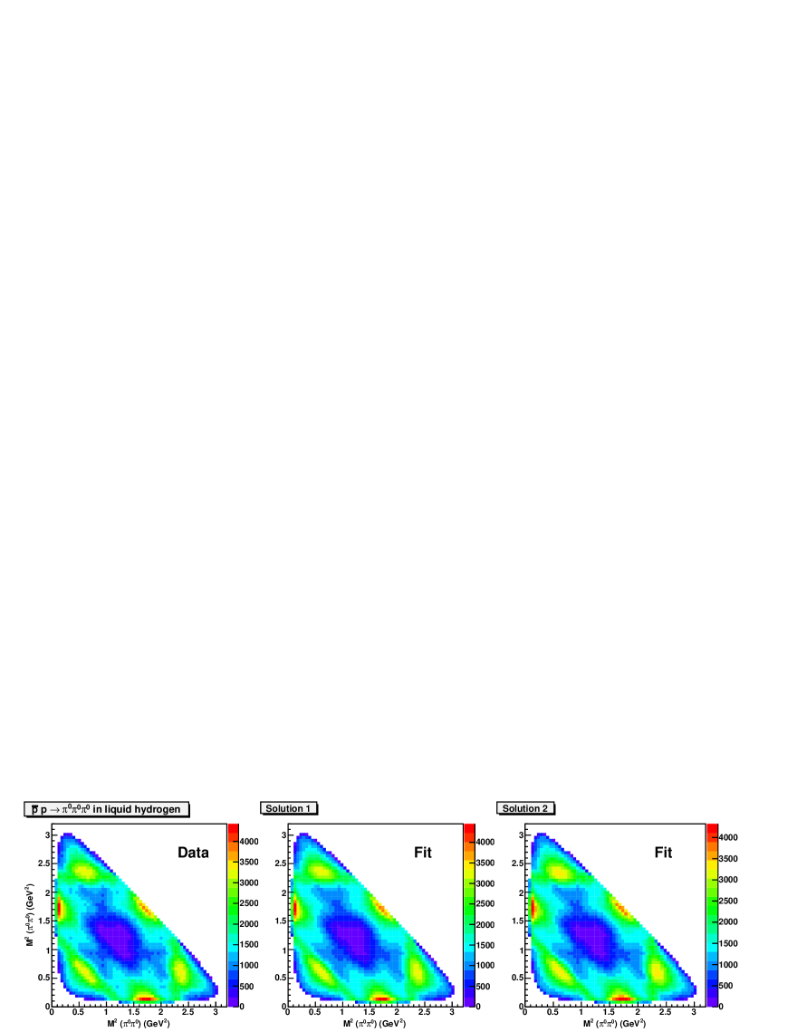
Figure 2: The acceptance-corrected Dalitz plot for the $p\bar{p}$ annihilation into $\pi^{0}\pi^{0}\pi^{0}$ in liquid $H_{2}$ and the result of the two solutions.

      

Figure 3: Mass projection of the acceptance-corrected Dalitz plot and angular distributions for specific mass slices. The data are taken from the $p\bar{p}$ annihilation into $3\pi^{0}$ in liquid $H_{2}$. Solid curves correspond to the solution 1 and dashed curves to the solution 2.

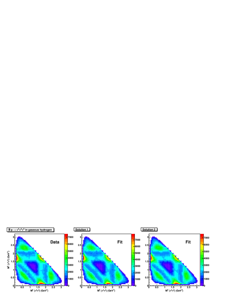
Figure 4: The acceptance-corrected Dalitz plot for the $p\bar{p}$ annihilation into $\pi^{0}\pi^{0}\pi^{0}$ in gaseous $H_{2}$ and the result of the two solutions.

      

Figure 5: Mass projection of the acceptance-corrected Dalitz plot and angular distributions for specific mass slices. The data are taken from the $p\bar{p}$ annihilation into $\pi^{0}\pi^{0}\pi^{0}$ in gaseous $H_{2}$. Solid curves correspond to the solution 1 and dashed curves to the solution 2.

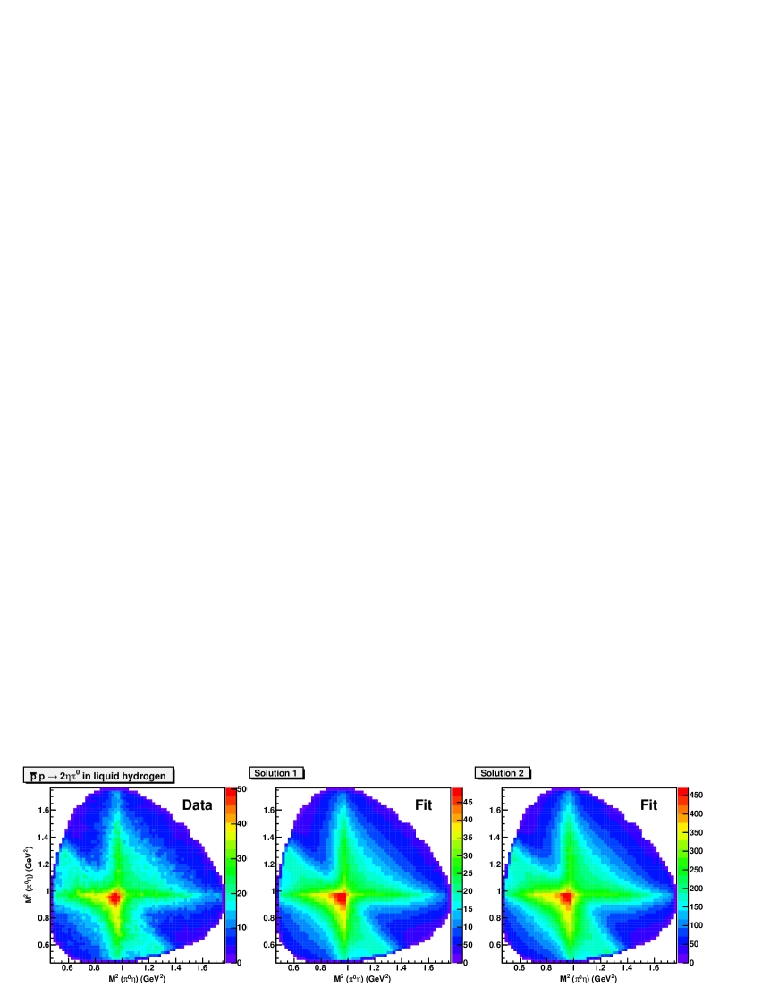
Figure 6: The acceptance-corrected Dalitz plot for the $p\bar{p}$ annihilation into $\eta\pi^{0}\eta$ in liquid $H_{2}$ and the result of the two solutions.

      

Figure 7: Mass projections of the acceptance-corrected Dalitz plot and angular distributions for specific mass slices. The data are taken from the $p\bar{p}$ annihilation into $\eta\pi^{0}\eta$ in liquid $H_{2}$. Solid curves correspond to the solution 1 and dashed curves to the solution 2.

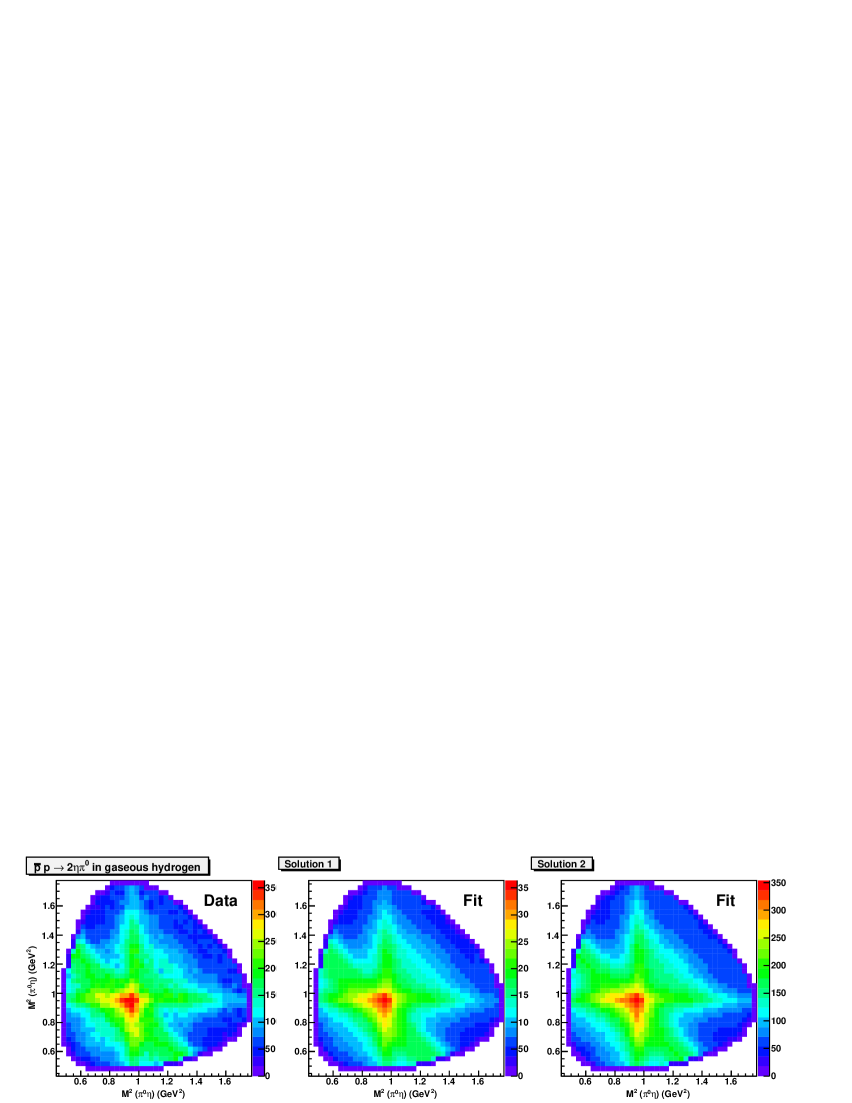
Figure 8: The acceptance-corrected Dalitz plot for the $p\bar{p}$ annihilation into $\eta\pi^{0}\eta$ in gaseous $H_{2}$ and the result of the two solutions.

      

Figure 9: Mass projections of the acceptance-corrected Dalitz plot and angular distributions for specific mass slices. The data are taken from the $p\bar{p}$ annihilation into $\eta\pi^{0}\eta$ in gaseous $H_{2}$. Solid curves correspond to the solution 1 and dashed curves to the solution 2.

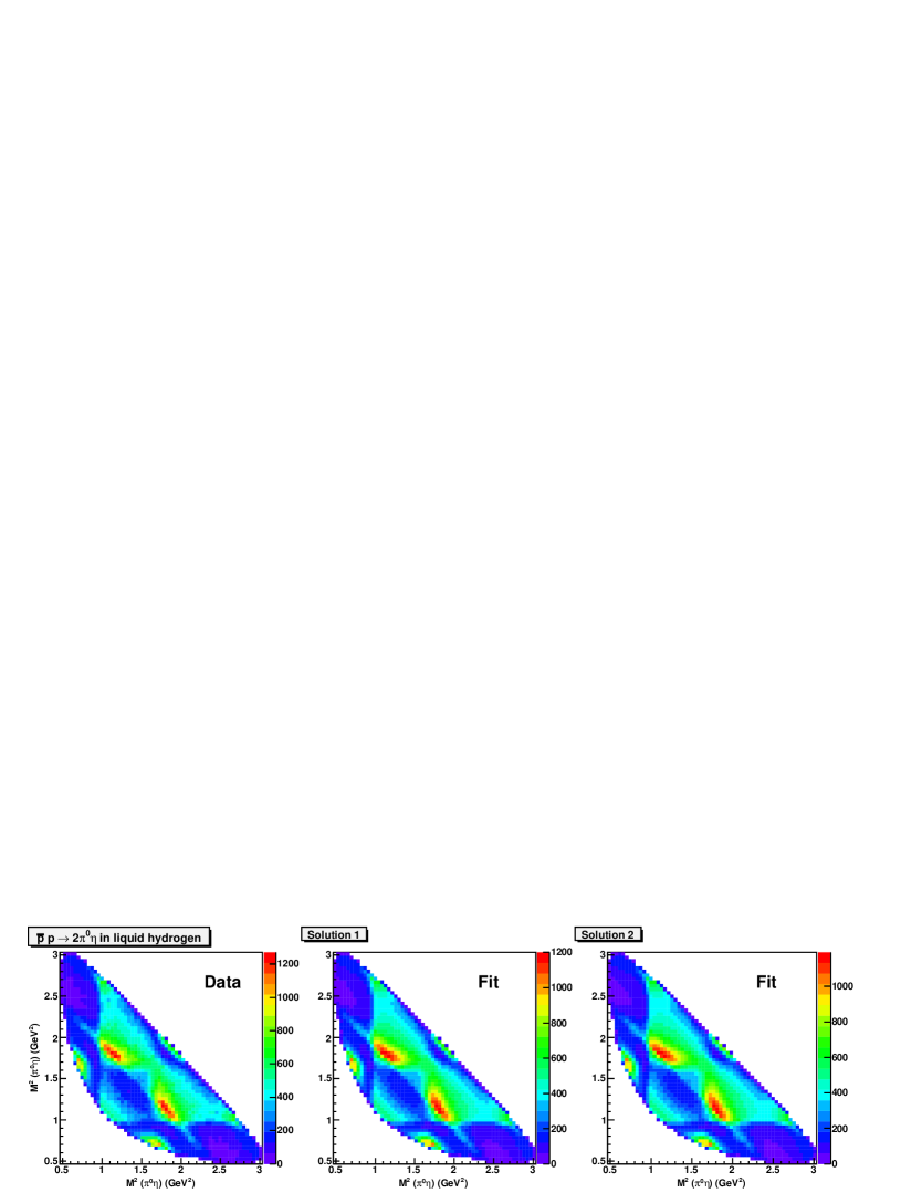
Figure 10: The acceptance-corrected Dalitz plot for the $p\bar{p}$ annihilation into $\pi^{0}\pi^{0}\eta$ in liquid $H_{2}$ and the result of the two solutions.

      

Figure 11: Mass projections of the acceptance-corrected Dalitz plot and angular distributions for specific mass slices. The data are taken from the $p\bar{p}$ annihilation into $\pi^{0}\pi^{0}\eta$ in liquid $H_{2}$. Solid curves correspond to the solution 1 and dashed curves to the solution 2.

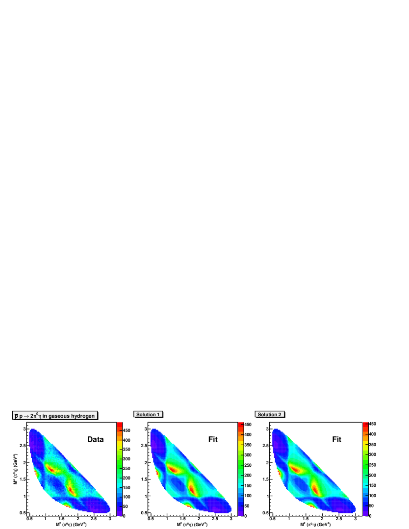
Figure 12: The acceptance-corrected Dalitz plot for the $p\bar{p}$ annihilation into $\pi^{0}\pi^{0}\eta$ in gaseous $H_{2}$ and two solutions.

      

Figure 13: Mass projections of the acceptance-corrected Dalitz plot and angular distributions for specific mass slices. The data are taken from the $p\bar{p}$ annihilation into $\pi^{0}\pi^{0}\eta$ in gaseous $H_{2}$. Solid curves correspond to the solution 1 and dashed curves to the solution 2.

Figure 14: Solution 1. The contributions of S-wave (two left columns) and D-wave (three right columns) to $Y_{00}$ moment integrated over $t$ intervals. First line: $-0.1\!<t\!<\!-0.01$ GeV², second line: $-0.2\!<\!t\!<\!-0.1$ GeV², third line: $-0.4\!<\!t\!<\!-0.2$ GeV² and the bottom line: $-0.4\!<\!t\!<\!-1.5$ GeV².

Figure 15: Solution 2. The contributions of S-wave (two left columns) and D-wave (three right columns) to $Y_{00}$ moment integrated over $t$ intervals. First line: $-0.1\!<\!t\!<\!-0.01$ GeV², second line: $-0.2\!<\!t\!<\!-0.1$ GeV², third line: $-0.4\!<\!t\!<\!-0.2$ GeV² and the bottom line: $-0.4\!<\!t\!<\!-1.5$ GeV².

4.2 The $K$-matrix fit of high-energy meson production: the $\pi$- and $a_{1}$-trajectory exchanges

The leading contribution from the $\pi$-exchange trajectory can contribute only to the moments with $m=0$, while the $a_{1}$-exchange can contribute to the moments up to $m=2$. The characteristic feature of the $a_{1}$ exchange is that moments with $m=2$ are suppressed compared to moments with $m=1$ by the ratio $k_{3x}/k_{3z}$ which is small for the system of two final mesons propagating with a large momentum in the beam direction.

The amplitudes defined by the $\pi$ and $a_{1}$ exchanges are orthogonal if the nucleon polarisation is not measured. This is due to the fact that the pion trajectory states are defined by the singlet combination of the nucleon spins while the $a_{1}$ trajectory states are defined by the triplet combination. This effect is not taken into account for the S-wave contribution in (9) which can lead to a misidentification of this wave at large momenta transferred.

The $\pi_{2}$ particle is situated on the pion trajectory and therefore should be described by the reggeized pion exchange. However, the $\pi_{2}$-exchange has next-to-leading order contributions with spherical functions at $m\geq 1$. The interference of such amplitudes with the pion exchange can be important (especially at small t) and is taken into account in the present analysis.

4.3 Results of the fit

To reconstruct the total cross section of the reaction $\pi^{-}p\to\pi^{0}\pi^{0}n$ which is not available to us we have used two partial wave decompositions provided by the E852 collaboration [17]. The cross section was reconstructed by Eq. (9) and decomposed over moments. The two partial wave decompositions produced very close results for the moments and we included the small differences between them as systematical errors.

The $\pi^{-}p\to\pi^{0}\pi^{0}n$ moments can be described successfully with only $\pi$, $a_{1}$ and $\pi_{2}$ leading trajectories taken into account and a simple assumption about the $t$-dependence of form factor for all partial waves. Moreover, we have found two solutions which differ by their contributions from these exchanges. Such an ambiguity is likely to be connected with the lack of polarisation data and can be resolved by data from future experiments.

The quality of the description of the Crystal Barrel data by both solutions is shown in Figs. 3-13 and the $\chi^{2}$ is given in Table 1. Here we also provide $\chi^{2}$ values for the $\pi\pi\to\eta\eta$ and $\pi\pi\to\eta\eta^{\prime}$ S-wave extracted by the GAMS collaboration [12],[13] from the $\pi^{-}N$ data taken at small transfer energies. It is seen that both solutions describe Crystal Barrel and GAMS data with the same quality. The main reason that the K-matrix parameters for the S and D-waves as well as P-vectors for the $\bar{p}p$ annihilation into three mesons are very similar in the two solutions. However the P-vectors for description of the E852 data are different in solutions 1 and 2.

Figure 16: The description of the moments extracted at $-0.1\!<\!t\!<\!-0.01$ GeV² (the left two columns) and $-0.2\!<\!t\!<\!-0.1$ GeV² (the right two columns). Dashed curves correspond to the solution 1 and full curves to the solution 2.

Figure 17: The description of the moments extracted at $-0.4\!<\!t\!<\!-0.2$ GeV² (two left columns) and $-1.5\!<\!t\!<\!-0.4$ GeV² (two right columns). Dashed curves correspond to the solution 1 and full lines to the solution 2.

In a more detail: these two solutions differ by the fraction of the $\pi$, $a_{1}$ and $\pi_{2}$ exchanges already in the region of small energy transferred. The first solution has a very large, practically dominant contribution from the $a_{1}$ exchange to the $D$-wave (see Fig. 14). The contribution from the $a_{1}$ exchange to the $S$-wave is small. In this solution there is no notable signal from the $f_{0}(1300)$ state either at small or at large energy transferred. If $f_{0}(1300)$ is excluded from this solution, only the description of the Crystal Barrel and GAMS data is deteriorated while the description of the E852 data has the same quality.

In the second solution the D-wave at small energies transferred is dominantly produced from the $\pi$ exchange. The fraction $a_{1}$ exchange at $|t|<0.1$ is about $2.5-3\%$. At large energy transferred, like in solution 1, the contribution from $a_{1}$ exchange becomes comparable and even dominant. The S-wave has a well known structure at small $|t|$. At intermediate energies the contribution from the $a_{1}$ exchange becomes dominant and a signal from the $f_{0}(1300)$ state is well seen in this wave. At very large $|t|$ ($-1.5<t<-0.4$ GeV²) the contribution from $a_{1}$ exchange is rather small. The dominant contribution comes from the $f_{0}(980)$ state produced from $\pi$ exchange. Here our analysis is in contradiction with the result reported by the E852 collaboration which observed a strong S-wave signal around 1300 MeV in this $t$-interval. However, the contribution from $f_{0}(1300)$ at intermediate energies transferred is important for the description of data with this solution. If this state is excluded from the fit the description is notably deteriorated, see Table 1, solution 2(-). This subject is considered in the following section in detail.

The Krakow group reported from the analysis of the polarized data that at small $t$ the dominant contribution comes from the $\pi$-exchange [30]. They point out that the second solution is possibly a physical one. However, the final conclusion can be made only after including these (yet unavailable to us) data in the present combined analysis which uses reggeon exchanges.

The description of the moments at small and large $|t|$ for the two solutions is shown in Figs. 16 and 17, correspondingly. The second solution produces a systematically better overall description except for the $Y^{1}_{4}$ moments at large energies transferred.

The S-wave was fitted to 5 poles in the 5-channel $K$-matrix, described in detail in previous sections. The parameters for the first solution are very close to those for the second one, e.g. the parametrization given in Table 2 describes both solutions, and the given errors cover a marginal change in both descriptions.

The D-wave was fitted to 4 poles in the 5-channel ($\pi\pi$, $K\bar{K}$, $\eta\eta$, $\omega\omega$ and $4\pi$) $K$-matrix. The position of the first two D-wave poles was found to be $1270-i97$ MeV and $1530-i72$ MeV which corresponds to the well-known resonances $f_{2}(1270)$ and $f_{2}(1525)$. The third state has a Flatté-structure near the $\omega\omega$ threshold and is defined by two poles on the sheets defined by the $\omega\omega$ cut. Due to the fact that we do not fit directly the $\omega\omega$ production data these positions can not be defined unambiguously. For example, in the framework of the solution 1 (dominant $a_{1}$-exchange in the D-wave) we found at least two solutions for the pole structure in the region of 1560 MeV. In the first the pole is situated at $1565-i140$ MeV on the sheet above the $\omega\omega$ threshold and $1690-i290$ MeV on the sheet below the $\omega\omega$ threshold. In the other solution the position of the pole is $1530-i262$ and $1699-i216$, correspondingly. The closest physical region is for both poles the beginning of the $\omega\omega$ threshold $M\sim$1570 MeV, where they form a relatively narrow (220–250 MeV) structure which is called the $f_{2}(1560)$ state, see Fig. 18. A similar situation was observed in the solution 2. The K-matrix D-wave parameters for the solution 2 are given in Table 3.

The fourth $D$-wave $K$-matrix pole, $f_{2}^{bare}(1980)$ cannot be rigidly fixed by the present data. The position of the corresponding pole is also not stable: one can easily increase the mass of the pole with the simultaneous increase of the width, spoiling only slightly the description of data. Because of that we consider this pole as some effective contribution of resonances located above 1900 MeV.

The $\pi\pi\to\pi\pi$ S-wave elastic amplitude for the second solution is shown in Fig.19. The structure of the amplitude is well known, it is defined by the destructive interference of the broad component with $f_{0}(980)$ and $f_{0}(1500)$. Neither $f_{0}(1300)$ nor $f_{0}(1750)$ provide a strong change of the amplitudes. However, this is hardly a surprise: both these states are relatively broad and dominantly inelastic.

Table 1: The $\chi^{2}$ per data point for the description of the Crystal Barrel and GAMS data. Two solutions are given as well as that with $f_{0}(1300)$ excluded from the fit, solution 2(-). For the E852 data the $\chi^{2}$ is calculated for all moments in the given $t$-interval

Data	Solution 1	Solution 2	Solution 2(-) (no $f_{0}(1300)$)
$\bar{p}p\to\pi^{0}\pi^{0}\pi^{0}$ (Liq)	1.360	1.356	1.443
$\bar{p}p\to\pi^{0}\pi^{0}\pi^{0}$ (Gas)	1.238	1.242	1.496
$\bar{p}p\to\eta\pi^{0}\eta$ (Liq)	1.350	1.442	1.446
$\bar{p}p\to\eta\pi^{0}\eta$ (Gas)	1.503	1.371	1.315
$\bar{p}p\to\pi^{0}\eta\pi^{0}$ (Liq)	1.210	1.236	1.412
$\bar{p}p\to\pi^{0}\eta\pi^{0}$(Gas)	1.099	1.119	1.227
$\pi\pi\to\eta\eta$ (S-wave)	1.08	1.19	1.38
$\pi\pi\to\eta\eta^{\prime}$ (S-wave)	0.26	0.41	0.45

Table 2: Masses and couplings (in GeV units) for the S-wave $K$-matrix poles ($f_{0}^{bare}$ states) as well as the amplitude pole positions (given in MeV). The II sheet is defined under the $\pi\pi$ and $4\pi$ cuts, the IV sheet is under $\pi\pi$, $4\pi$, $K\bar{K}$ and $\eta\eta$ cuts, and the V sheet is determined by $\pi\pi$, $4\pi$, $K\bar{K}$, $\eta\eta$ and $\eta\eta^{\prime}$ cuts.

	$\alpha=1$	$\alpha=2$	$\alpha=3$	$\alpha=4$	$\alpha=5$
M	$0.720^{+.50}_{-.080}$	$1.220^{+.040}_{-.030}$	$1.210\pm 030$	$1.550^{+.030}_{-.020}$	$1.850\pm.040$
$g_{0}^{(\alpha)}$	$0.760^{+.080}_{-.060}$	$0.820\pm 0.090$	$0.470\pm.050$	$0.360\pm.050$	$0.440\pm.050$
$g_{5}^{(\alpha)}$	0	0	$0.850\pm.100$	$0.570\pm.070$	$-0.900\pm.070$
$\varphi_{\alpha}$	-($60\pm 12$)	$28\pm 12$	$30\pm 14$	$8\pm 15$	-($52\pm 14$)
	$a=\pi\pi$	$a=K\bar{K}$	$a=\eta\eta$	$a=\eta\eta^{\prime}$	$a=4\pi$
$f_{1a}$	$0.180\pm.120$	$0.150\pm.100$	$0.240\pm.100$	$0.300\pm.100$	$0.0\pm.060$
		$f_{ba}=0$	$b=2,3,4,5$
		Pole position
II	$1030^{+30}_{-10}$
sheet	$-i(35^{+10}_{-16})$
III	$850^{+80}_{-50}$
sheet	$-i(100\pm 25)$
IV		$1290\pm 50$	$1486\pm 10$	$1510\pm 130$
sheet		$-i(170^{+20}_{-40})$	$-i(57\pm 5)$	$-i(800^{+100}_{-150})$
V					$1800\pm 60$
sheet					$-i(200\pm 30)$

Table 3: Masses and couplings (in GeV units) for $D$-wave $K$-matrix poles ($f_{2}^{bare}$ states) for the solution 2. The III sheet is defined by $\pi\pi$ and $4\pi$ and $K\bar{K}$ cuts, the IV sheet by $\pi\pi$, $4\pi$, $K\bar{K}$ and $\omega\omega$ cuts. The values marked by $*$ were fixed in the fit.

	$\alpha=1$	$\alpha=2$	$\alpha=3$	$\alpha=4$
M	$1.286\pm 0.025$	$1.540\pm 0.015$	$1.560\pm 0.020$	$2.200^{+0.300}_{-0.200}$
$g_{\pi\pi}^{(\alpha)}$	$0.920\pm 0.020$	$-0.05\pm 0.080$	$0.280\pm 0.100$	$-0.30\pm 0.15$
$g_{\eta\eta}^{(\alpha)}$	$0.420\pm 0.060$	$0.27\pm 0.15$	$0.400\pm 0.200$	$1.2\pm 0.6^{*}$
$g_{4\pi}^{(\alpha)}$	$-0.150\pm 0.200$	$0.370\pm 0.150$	$1.170\pm 0.450$	$1.0\pm 0.4$
$g_{\omega\omega}^{(\alpha)}$	$0^{*}$	$0^{*}$	$0.540\pm 0.150$	$-0.05\pm 0.2$
	$a=\pi\pi$	$a=\eta\eta$	$a=\omega\omega$	$a=4\pi$
$f_{1a}$	$0.03\pm 0.15$	$-0.11\pm 0.10$	$0^{*}$	$0^{*}$
$f_{2a}$	$-0.11\pm 0.10$	$-1.8\pm 0.60$	$0^{*}$	$0^{*}$
		$f_{ba}=0$	$b=3,4,5$
		Pole position
III sheet	$1.270\pm 0.008$	$1.530\pm 0.012$
	$-i\,0.097\pm 0.008$	-i$\,0.064\pm 0.010$
III sheet			$1.690\pm 0.015$
			$-i\,0.290\pm 0.020$
IV sheet			$1.560\pm 0.015$
			$-i\,0.140\pm 0.020$

         

Figure 18: Pole structure of the 2⁺⁺-amplitude in the region of the $\omega\omega$-threshold: the resonance $f_{2}(1560)$: a) solution 1(i), b) solution 1(ii)

Figure 19: From left to right: a) The $\pi\pi\to\pi\pi$ S-wave amplitude squared, b) the amplitude phase and c) the Argand diagram for the S-wave amplitude $\pi\pi\to\pi\pi$.

The $\pi\pi\to\pi\pi$ D-wave elastic amplitude is shown in Fig. 20. The amplitude squared is dominated by the $f_{2}(1270)$ state. Neither of $f_{2}(1560)$ and $f_{2}(1510)$ (which are included into the $K\bar{K}$ channel of the $K$-matrix) show a meaningful structure in the amplitude squared. The $K$-matrix parameters found in the solution are given in Table 3.

Figure 20: From left to right: The $\pi\pi\to\pi\pi$ D-wave amplitude squared, the amplitude phase and the Argand diagram for the amplitude.

4.4 The $f_{0}(1300)$ state

In the solution 2 the fit of the E852 data shows a large contribution from the $f_{0}(1300)$ state to $Y^{0}_{0}$ moment due to $a_{1}$ exchange at $-0.2\!<\!t\!<\!-0.1$ and $-0.4\!<\!t\!<\!-0.2$ GeV². At very small ($-0.1\!<\!t\!<\!-0.01$ GeV²) and large ($-1.5\!<\!t\!<\!-0.4$ GeV²) energy transferred the contribution of this state to the $Y^{0}_{0}$ moment is less pronounced. If the K-matrix pole which corresponds to the $f_{0}(1300)$ state is excluded from the fit (all couplings are put to zero) the total $\chi^{2}$ changes rather appreciably. The corresponding values for the description of the Crystal Barrel and GAMS data are given in the last column of Table 1 (solution 2(-)). The mass slices made in the region of the state show systematical discrepancies in this case (see Fig.21).

      

Figure 21: Angular distributions for specific mass slices. a) $\bar{p}p\to 3\pi^{0}$ (gas) b) $\bar{p}p\to\pi^{0}\eta\eta$ (liquid), c,d,e) $\bar{p}p\to\pi^{0}\eta\eta$ (gas). Solid curves correspond to the solution 2 and dashed curves to the solution 2(-) with excluded $f_{0}(1300)$.

For the description of the E852 data the main effect is seen, as expected, for the second and third $t$ intervals. The comparison of the solutions with and without $f_{0}(1300)$ for these $t$ regions is shown in Fig. 22. Here the description of the $Y^{1}_{4}$ moment is systematically worse for the fit where $f_{0}(1300)$ is excluded. The $\chi^{2}$ per data points change for this moment from 1.84 to 3.63 for the $-0.2\!<\!t\!<\!-0.1$ GeV² interval and from 2.07 to 4.90 for the $-0.4\!<\!t\!<\!-0.2$ GeV² interval. The fit without $f_{0}(1300)$ produces a worse description also for $Y^{0}_{2}$ and $Y_{4}^{0}$. At intervals of small and large $t$ the description has the same quality and can hardly be distinguished on the pictures. The contribution of the S-wave to the moment $Y^{0}_{0}$ from this solution is shown in Fig. 23. It is seen that an appreciable contribution from $a_{1}$ exchange at the mass region 1300-1500 MeV is needed and the fit tries to simulate it (although not very successfully) by an interference between the broad component and the $f_{0}(1500)$ state.

Figure 22: The description of the moments extracted at $-0.1\!<\!t\!<\!-0.2$ GeV² (two left columns) and $-0.4\!<\!t\!<\!-0.2$ GeV² (two right columns). Solid curves correspond to the solution 2 and dashed line to the solution 2(-) with excluded $f_{0}(1300)$.

Figure 23: Solution 2(-) with $f_{0}(1300)$ excluded from the fit. The contributions of S-wave to $Y_{00}$ moment integrated over different $t$ intervals. First line: $t\!<\!-0.1$ GeV², second line: $-0.1\!<\!t\!<\!-0.2$ GeV², third line: $-0.2\!<\!t\!<\!-0.4$ GeV² and the bottom line: $-1.5\!<\!t\!<\!-0.4$ GeV².

Below we present the pole positions of the S-wave amplitude (in MeV units) and couplings calculated as pole residues (in GeV units): $A_{a\to b}\simeq G_{a}G_{b}[(M-i\Gamma/2)^{2}-s]^{-1}+smooth\,terms$ with $a,b=\pi\pi,K\bar{K},\eta\eta,\eta\eta^{\prime},\pi\pi\pi\pi$; the couplings are written as $G_{a}=g_{a}\exp(i\varphi_{a})$, the phases are given in degrees. For resonances $f_{0}(980)$, $f_{0}(1300)$, $f_{0}(1500)$, $f_{0}(1200-1600)$, $f_{0}(1750)$ we obtain:

$$f_{0}(980)_{1st\,pole}$$

M

Sheet II III IV IV IV V

(69)

4.5 Isovector scalar and tensor resonances below 1.7 GeV

The isovector states are contributing strongly to the $\bar{p}p\to\eta\eta\pi^{0}$ and $\bar{p}p\to\pi^{0}\pi^{0}\eta$ amplitude.

The $a_{0}(980)$ is clearly seen on the $\eta\eta\pi^{0}$ Dalitz plot and on the $\pi\eta$ mass projection. A successful description of these data can be obtained with the Flatté parametrization of this resonance (pole parametrization with decays into channels $\pi\eta$ and $K\bar{K}$). Within this parametrization (for more detail see [31]) we obtain the following masses and couplings for $a_{0}(980)$:

M (MeV) $$g^{2}_{\pi\eta}$$ (GeV)

(70)

These parameters result in the following two poles on the I-st sheet (under the $\pi\eta$ cut) and the II-nd sheet (under the $\pi\eta$ and $K\bar{K}$ cuts) for $a_{0}(980)$:

I-st sheet II-nd sheet

$$1000\pm 6\!-\!i(35\pm 4)$$ MeV, MeV

(71)

The second isovector scalar state $a_{0}(1474)$ [1] (defined as $a_{0}(1450)$ in PDG) is situated in the 1500 MeV region. We found:

$${\rm\,Pole\,position\,of\,}a_{0}(1474):\qquad M=1515\pm 30-i(115\pm 18)\quad{\rm MeV}.$$ (72)

This state is highly inelastic with a branching ratio into the $\pi\eta$ channel less than $10\%$. We have not found any indications for an extra isovector scalar state in the mass region between $a_{0}(980)$ and $a_{0}(1474)$.

The resonance $a_{2}(1320)$ contributes to the $\bar{p}p\to\pi^{0}\pi^{0}\eta$ strongly, here we see also $a_{2}(1675)$-signal. We parametrized these resonances in the Breit-Wigner form and have found the following amplitude poles:

$$a_{2}(1320)$$

MeV, MeV

(73)

For $a_{2}(1320)$ we have found a mass $1309\pm 4$ MeV which is lower by 9 MeV than the average PDG value but corresponds very well to the analysis of high statistical data performed by the VES collaboration [39]. The observed width of the state $111\pm 4$ corresponds well to other observations from the $\pi\eta$ decay mode.

The $a_{2}(1675)$ state improves the fit; however, the mass and width of this state can not be well defined from these data because the resonance is situated on the phase volume boundary and is suppressed by the D-wave centrifugal barrier. The obtained values are compatible with previous findings of the Crystal Barrel collaboration [34]. Let us mention that the mass and width of this state can be much better defined from the L3 data on $\gamma\gamma$ interaction into $\pi^{+}\pi^{-}\pi^{0}$ [35].

5 Summary for isoscalar resonances

We develop a method for the analysis of the reactions $\pi N\to two\,mesons+N$ at large energies of the initial pion. The approach is based on the use of the reggeized exchanges that allow us to analyze simultaneously the data obtained at small and large momentum transfers. In the present article the method is applied to the analysis of the $\pi^{-}N\to\pi^{0}\pi^{0}N$ data measured by the E852 experiment. The inclusion of the Crystal Barrel data on the proton-antiproton annihilation at rest into the $3\pi^{0}$, $\pi^{0}\eta\eta$ and $\pi^{0}\pi^{0}\eta$ channels helps to reduce ambiguities in the isoscalar sector and investigate the properties of the isovector scalar and tensor states.

As the result of the analysis the K-matrix parameters of the isoscalar-scalar and isoscalar-tensor states was obtained up to the invariant mass 2 GeV and pole positions of corresponding amplitudes are defined.

5.1 Isoscalar-scalar sector

In the scalar sector the contribution of the $f_{0}(1300)$ is necessary to get a consistent description for the data set analyzed:

$${\rm\,Pole\,position\,of\,}f_{0}(1300):\qquad M=1290\pm 50-i(170^{+20}_{-40})\quad{\rm MeV}.$$ (74)

According to our fit, the strong signal in the $\pi\pi$ spectrum in the region 1300 MeV is formed by two contributions, by $f_{0}(1300)$ (dominantly the $a_{1}$ reggeized exchange) and $f_{2}(1275)$ (the $\pi$ and $a_{1}$ reggeized exchanges).

The position of the $f_{0}(980)$ is defined very well. The resonance reveals a double pole structure around the $K\bar{K}$ threshold.

$${\rm\,Pole\,positions\,of\,}f_{0}(980):$$ (75)

$${\rm\,sheet\,II\,(under\,\pi\pi\,and\,\pi\pi\pi\pi\,cuts)}:\qquad M=1030^{+30}_{-10}-i(35^{+10}_{-16})\quad{\rm MeV},$$

$${\rm\,sheet\,III\,(under\,\pi\pi,\,\pi\pi\pi\pi\,and\,K\bar{K}\,cuts)}:\qquad M=850^{+80}_{-50}-i(200\pm 50)\quad{\rm MeV}.$$

The $f_{0}(1500)$ is defined from the combined fit with a good accuracy:

$${\rm\,Pole\,position\,of\,}f_{0}(1500):\qquad M=1486\pm 10-i(57\pm 5)\quad{\rm MeV}.$$ (76)

The broad state $f_{0}(1200-1600)$ (the scalar glueball descendant) gives contribution in $\pi\pi$ scattering amplitudes in region up to 2 GeV; the following pole position is found

$${\rm\,Pole\,position\,of\,}f_{0}(1200-1600):\qquad M=(1510\pm 130)-i(800^{+100}_{-150})\quad{\rm MeV}.$$ (77)

The $f_{0}(1750)$ is a dominantly $s\bar{s}$ state [1] and is needed to describe $\pi\pi\to\pi\pi$ and $\pi\pi\to\eta\eta$ amplitudes above 1750 MeV.

$${\rm\,Pole\,position\,of\,}f_{0}(1750):\qquad M=1800\pm 60-i(200\pm 30)\quad{\rm MeV}.$$ (78)

Parameters of this state differ from that observed by the BES [36] and WA102 [37] collaborations (denoted as $f_{0}(1710)$); one should, however, have in mind that in the case of strong interferences characteristics of a peak in the data does not correspond to the resonance position. A combined fit of the Crystal Barrel, CERN-Munich, E852, GAMS and BES data is needed and it is one of our future objectives.

5.2 Isoscalar-tensor sector

The D-wave reveals the resonances $f_{2}(1275)$, $f_{2}(1525)$, $f_{2}(1565)$, and $f_{2}(1950)$ with the following pole positions:

$$f_{2}(1275) :\qquad M=1270\pm 8-i(97\pm 8)\,{\rm MeV},$$

$$f_{2}(1525) :\qquad M=1530\pm 12-i(64\pm 10)\,{\rm MeV},$$

$$f_{2}(1565)\;{\rm(2nd\,solution)} :\qquad M_{I}=1690\pm 15-i(290\pm 20)\,{\rm MeV},$$ (79)

$$M_{II}=1560\pm 15-i(140\pm 20)\,{\rm MeV},$$

In the case of $f_{2}(1565)$ the K-matrix fit can be obtained only with the large coupling of this state to $\omega\omega$ (and, possibly, to $\rho\rho$) channel (note that this result is in a very good agreement with the analysis of the proton-antiproton annihilation into $\omega\omega\pi$ [38]). The large coupling to $\omega\omega$ leads to the double pole structure of $f_{2}(1565)$, see Fig. 18.

The state $f_{2}(1980)$ can not be identified unambiguously from the present data due to its large inelasticity. It plays the role of some broad contribution needed for the description of the $\pi N$ data

5.3 Isoscalar sector $J^{PC}=4^{++}$

For the description of high moments in the $\pi N\to\pi^{0}\pi^{0}N$ data a contribution from a $4^{++}$ state is needed. This state is identified as $f_{4}(2025)$. Due to the lack of data at high masses this state was fitted as a two channel ($\pi\pi$ and $4\pi$) one pole K-matrix.

M (GeV) $$g_{\pi\pi}$$

(80)

Here, as previously, masses and couplings are in GeV units. The position of the pole is equal to $(1966\pm 25)-i\,(130\pm 20)$. The amplitude phase and the Argand diagram for the isoscalar $4^{++}$ state is shown in Fig.24. The $\pi\pi\to\pi\pi$ $4^{++}$ amplitude has a peak at 1995 MeV and is slightly asymmetrical: the half height is reached at the mass 1880 and 2165 MeV. The branching ratio of the $\pi\pi$ channel at the pole position is $20\pm 3\%$ which is in agreement with the PDG value within the error.

Figure 24: From left to right: The $\pi\pi\to\pi\pi$ G-wave amplitude squared, the amplitude phase and the Argand diagram for the amplitude.

6 Appendix A. Angular Momentum Operators

The angular-dependent part of the wave function of a composite state is described by operators constructed for the relative momenta of particles and the metric tensor. Such operators (we denote them as $X^{(L)}_{\mu_{1}\ldots\mu_{L}}$, where $L$ is the angular momentum) are called angular momentum operators; they correspond to irreducible representations of the Lorentz group. They satisfy the following properties:
(i) Symmetry with respect to the permutation of any two indices:

$$X^{(L)}_{\mu_{1}\ldots\mu_{i}\ldots\mu_{j}\ldots\mu_{L}}\;=\;X^{(L)}_{\mu_{1}\ldots\mu_{j}\ldots\mu_{i}\ldots\mu_{L}}.$$ (81)

(ii) Orthogonality to the total momentum of the system, $P=k_{1}+k_{2}$:

$$P_{\mu_{i}}X^{(L)}_{\mu_{1}\ldots\mu_{i}\ldots\mu_{L}}\ =\ 0.$$ (82)

(iii) Tracelessness with respect to the summation over any two indices:

$$g_{\mu_{i}\mu_{j}}X^{(L)}_{\mu_{1}\ldots\mu_{i}\ldots\mu_{j}\ldots\mu_{L}}\ \ =\ 0.$$ (83)

Let us consider a one-loop diagram describing the decay of a composite system into two spinless particles, which propagate and then form again a composite system. The decay and formation processes are described by angular momentum operators. Owing to the quantum number conservation, this amplitude must vanish for initial and final states with different spins. The S-wave operator is a scalar and can be taken as a unit operator. The P-wave operator is a vector. In the dispersion relation approach it is sufficient that the imaginary part of the loop diagram, with S- and P-wave operators as vertices, equals 0. In the case of spinless particles, this requirement entails

$$\int\frac{d\Omega}{4\pi}X^{(1)}_{\mu}=0\ ,$$ (84)

where the integral is taken over the solid angle of the relative momentum. In general, the result of such an integration is proportional to the total momentum $P_{\mu}$ (the only external vector):

$$\int\frac{d\Omega}{4\pi}X^{(1)}_{\mu}=\lambda P_{\mu}\;.$$ (85)

Convoluting this expression with $P_{\mu}$ and demanding $\lambda=0$, we obtain the orthogonality condition (82). The orthogonality between the D- and S-waves is provided by the tracelessness condition (83); equations (82), (83) provide the orthogonality for all operators with different angular momenta.

The orthogonality condition (82) is automatically fulfilled if the operators are constructed from the relative momenta $k^{\perp}_{\mu}$ and tensor $g^{\perp}_{\mu\nu}$. Both of them are orthogonal to the total momentum of the system:

$$k^{\perp}_{\mu}=\frac{1}{2}g^{\perp}_{\mu\nu}(k_{1}-k_{2})_{\nu}\ ,\qquad g^{\perp}_{\mu\nu}=g_{\mu\nu}-\frac{P_{\mu}P_{\nu}}{s}\;.$$ (86)

In the c.m. system, where $P=(P_{0},\vec{P})=(\sqrt{s},0)$, the vector $k^{\perp}$ is space-like: $k^{\perp}=(0,\vec{k},0)$.

The operator for $L=0$ is a scalar (for example, a unit operator), and the operator for $L=1$ is a vector, which can be constructed from $k^{\perp}_{\mu}$ only. The orbital angular momentum operators for $L=0$ to 3 are:

$$X^{(0)}(k^{\perp})=1,\qquad X^{(1)}_{\mu}=k^{\perp}_{\mu},$$ (87)

$$X^{(2)}_{\mu_{1}\mu_{2}}(k^{\perp})=\frac{3}{2}\left(k^{\perp}_{\mu_{1}}k^{\perp}_{\mu_{2}}-\frac{1}{3}\,k^{2}_{\perp}g^{\perp}_{\mu_{1}\mu_{2}}\right),$$

$$X^{(3)}_{\mu_{1}\mu_{2}\mu_{3}}(k^{\perp})=\frac{5}{2}\Big{[}k^{\perp}_{\mu_{1}}k^{\perp}_{\mu_{2}}k^{\perp}_{\mu_{3}}-\frac{k^{2}_{\perp}}{5}\left(g^{\perp}_{\mu_{1}\mu_{2}}k^{\perp}_{\mu_{3}}+g^{\perp}_{\mu_{1}\mu_{3}}k^{\perp}_{\mu_{2}}+g^{\perp}_{\mu_{2}\mu_{3}}k^{\perp}_{\mu_{1}}\right)\Big{]}.$$

The operators $X^{(L)}_{\mu_{1}\ldots\mu_{L}}$ for $L\geq 1$ can be written in the form of a recurrency relation:

$$X^{(L)}_{\mu_{1}\ldots\mu_{L}}(k^{\perp}) = k^{\perp}_{\alpha}Z^{\alpha}_{\mu_{1}\ldots\mu_{L}}(k^{\perp})\;,$$

$$Z^{\alpha}_{\mu_{1}\ldots\mu_{L}}(k^{\perp}) = \frac{2L-1}{L^{2}}\Big{(}\sum^{L}_{i=1}X^{{(L-1)}}_{\mu_{1}\ldots\mu_{i-1}\mu_{i+1}\ldots\mu_{L}}(k^{\perp})g^{\perp}_{\mu_{i}\alpha}$$

$$-\frac{2}{2L-1}\sum^{L}_{i,j=1\atop i<j} g^{\perp}_{\mu_{i}\mu_{j}} X^{{(L-1)}}_{\mu_{1}\ldots\mu_{i-1}\mu_{i+1}\ldots\mu_{j-1}\mu_{j+1}\ldots\mu_{L}\alpha}(k^{\perp})\Big{)}.$$ (88)

The convolution equality reads

$$X^{(L)}_{\mu_{1}\ldots\mu_{L}}(k^{\perp})k^{\perp}_{\mu_{L}}=k^{2}_{\perp}X^{(L-1)}_{\mu_{1}\ldots\mu_{L-1}}(k^{\perp}).$$ (89)

On the basis of Eq.(89) and taking into account the tracelessness property of $X^{(L)}_{\mu_{1}\ldots\mu_{L}}$, one can write down the orthogonality–normalisation condition for orbital angular operators

$$\int\frac{d\Omega}{4\pi}X^{(L)}_{\mu_{1}\ldots\mu_{L}}(k^{\perp})X^{(L^{\prime})}_{\mu_{1}\ldots\mu_{L}^{\prime}}(k^{\perp})\ =\ \delta_{LL^{\prime}}\alpha_{L}k^{2L}_{\perp}\;,$$

$$\alpha_{L}\ =\ \prod^{L}_{l=1}\frac{2l-1}{l}\;.$$ (90)

Iterating equation (88), one obtains the following expression for the operator $X^{(L)}_{\mu_{1}\ldots\mu_{L}}$:

$$X^{(L)}_{\mu_{1}\ldots\mu_{L}}(k^{\perp})=\alpha_{L}\bigg{[}k^{\perp}_{\mu_{1}}k^{\perp}_{\mu_{2}}k^{\perp}_{\mu_{3}}k^{\perp}_{\mu_{4}}\ldots k^{\perp}_{\mu_{L}}$$

$$-\frac{k^{2}_{\perp}}{2L-1}\bigg{(}g^{\perp}_{\mu_{1}\mu_{2}}k^{\perp}_{\mu_{3}}k^{\perp}_{\mu_{4}}\ldots k^{\perp}_{\mu_{L}}+g^{\perp}_{\mu_{1}\mu_{3}}k^{\perp}_{\mu_{2}}k^{\perp}_{\mu_{4}}\ldots k^{\perp}_{\mu_{L}}+\ldots\bigg{)}$$

$$+\frac{k^{4}_{\perp}}{(2L\!-\!1)(2L\!-\!3)}\bigg{(}g^{\perp}_{\mu_{1}\mu_{2}}g^{\perp}_{\mu_{3}\mu_{4}}k^{\perp}_{\mu_{5}}k^{\perp}_{\mu_{6}}\ldots k^{\perp}_{\mu_{L}}$$

$$+g^{\perp}_{\mu_{1}\mu_{2}}g^{\perp}_{\mu_{3}\mu_{5}}k^{\perp}_{\mu_{4}}k^{\perp}_{\mu_{6}}\ldots k^{\perp}_{\mu_{L}}+\ldots\bigg{)}+\ldots\bigg{]}.$$ (91)

The projection operator $O^{\mu_{1}\ldots\mu_{L}}_{\nu_{1}\ldots\nu_{L}}$ (or $O^{\mu_{1}\ldots\mu_{L}}_{\nu_{1}\ldots\nu_{L}}(\perp P)$) is constructed of the metric tensors $g^{\perp}_{\mu\nu}$. It has the properties as follows:

$$X^{(L)}_{\mu_{1}\ldots\mu_{L}}O^{\mu_{1}\ldots\mu_{L}}_{\nu_{1}\ldots\nu_{L}}\ = \ X^{(L)}_{\nu_{1}\ldots\nu_{L}}\ ,$$

$$O^{\mu_{1}\ldots\mu_{L}}_{\alpha_{1}\ldots\alpha_{L}}\ O^{\alpha_{1}\ldots\alpha_{L}}_{\nu_{1}\ldots\nu_{L}}\ = O^{\mu_{1}\ldots\mu_{L}}_{\nu_{1}\ldots\nu_{L}}\ .$$ (92)

Taking into account the definition of projection operators (92) and the properties of the $X$-operators (6), we obtain

$$k_{\mu_{1}}\ldots k_{\mu_{L}}O^{\mu_{1}\ldots\mu_{L}}_{\nu_{1}\ldots\nu_{L}}\ =\frac{1}{\alpha_{L}}X^{(L)}_{\nu_{1}\ldots\nu_{L}}(k^{\perp}).$$ (93)

This equation is the basic property of the projection operator: it projects any operator with $L$ indices onto the partial wave operator with angular momentum $L$.

For the lowest states,

$$O=1\ ,\qquad O^{\mu}_{\nu}=g_{\mu\nu}^{\perp}\,,$$

$$O^{\mu_{1}\mu_{2}}_{\nu_{1}\nu_{2}}=\frac{1}{2}\left(g_{\mu_{1}\nu_{1}}^{\perp}g_{\mu_{2}\nu_{2}}^{\perp}\!+\!g_{\mu_{1}\nu_{2}}^{\perp}g_{\mu_{2}\nu_{1}}^{\perp}\!-\!\frac{2}{3}g_{\mu_{1}\mu_{2}}^{\perp}g_{\nu_{1}\nu_{2}}^{\perp}\right).\;\;$$ (94)

For higher states, the operator can be calculated using the recurrent expression:

$$O^{\mu_{1}\ldots\mu_{L}}_{\nu_{1}\ldots\nu_{L}}=\frac{1}{L^{2}}\bigg{(}\sum\limits_{i,j=1}^{L}g^{\perp}_{\mu_{i}\nu_{j}}O^{\mu_{1}\ldots\mu_{i-1}\mu_{i+1}\ldots\mu_{L}}_{\nu_{1}\ldots\nu_{j-1}\nu_{j+1}\ldots\nu_{L}}$$ (95)

$$-\frac{4}{(2L-1)(2L-3)}\times\sum\limits_{i<j\atop k<m}^{L}g^{\perp}_{\mu_{i}\mu_{j}}g^{\perp}_{\nu_{k}\nu_{m}}O^{\mu_{1}\ldots\mu_{i-1}\mu_{i+1}\ldots\mu_{j-1}\mu_{j+1}\ldots\mu_{L}}_{\nu_{1}\ldots\nu_{k-1}\nu_{k+1}\ldots\nu_{m-1}\nu_{m+1}\ldots\nu_{L}}\bigg{)}.$$

The product of two $X$-operators integrated over a solid angle (that is equivalent to the integration over internal momenta) depends only on the external momenta and the metric tensor. Therefore, it must be proportional to the projection operator. After straightforward calculations we obtain

$$\!\!\!\int\!\frac{d\Omega}{4\pi}\!X^{(L)}_{\mu_{1}\ldots\mu_{L}}(k^{\perp})X^{(L)}_{\nu_{1}\ldots\nu_{L}}(k^{\perp})\!=\!\frac{\alpha_{L}\,k^{2L}_{\perp}}{2L\!+\!1}O^{\mu_{1}\ldots\mu_{L}}_{\nu_{1}\ldots\nu_{L}}\ .$$ (96)

Let us introduce the positive valued $|\vec{k}|^{2}$:

$$|\vec{k}|^{2}\!=\!-k_{\perp}^{2}\!=\!\frac{[s\!-\!(m_{1}\!+\!m_{2})^{2}][s\!-\!(m_{1}\!-\!m_{2})^{2}]}{4s}\ .$$ (97)

In the c.m.s. of the reaction, $\vec{k}$ is the momentum of a particle. In other systems we use this definition only in the sense of $|\vec{k}|\equiv\sqrt{-k_{\perp}^{2}}$; clearly, $|\vec{k}|^{2}$ is a relativistically invariant positive value. If so, equation (96) can be written as

$$\int\!\frac{d\Omega}{4\pi}\!X^{(L)}_{\mu_{1}\ldots\mu_{L}}(k^{\perp})X^{(L)}_{\nu_{1}\ldots\nu_{L}}(k^{\perp})\!=\!\frac{\alpha_{L}\,|\vec{k}|^{2L}}{2L\!+\!1}(-1)^{L}O^{\mu_{1}\ldots\mu_{L}}_{\nu_{1}\ldots\nu_{L}}.$$ (98)

The tensor part of the numerator of the boson propagator is defined by the projection operator. Let us write it as follows:

$$F^{\mu_{1}\ldots\mu_{L}}_{\nu_{1}\ldots\nu_{L}}=(-1)^{L}\,O^{\mu_{1}\ldots\mu_{L}}_{\nu_{1}\ldots\nu_{L}}\ ,$$ (99)

with the definition of the propagator

$$\frac{F^{\mu_{1}\ldots\mu_{L}}_{\nu_{1}\ldots\nu_{L}}}{M^{2}-s}.$$ (100)

This definition guarantees that the width of a resonance (calculated using the decay vertices) is positive.

References

• [1] A.V. Anisovich, V.V. Anisovich, J. Nyiri, V.A. Nikonov, M.A. Matveev and A.V. Sarantsev, ”Mesons and Baryons”, World Scientific, Singapore, 2008.
• [2] B.Β Hyams et al., Nucl.Β Phys.Β  B 64 (1973) 134 [AIP Conf.Β Proc.Β  13 (1973) 206].
• [3] A. Etkin, et al., Phys. Rev. D 25, 1786 (1982).
• [4] S.Β U.Β Chung, Phys.Β Rev.Β  D 56 (1997) 7299.
• [5] V.V. Anisovich and A.V. Sarantsev, Phys. Lett. B 382, 429 (1996).
• [6] V.V. Anisovich, D.V. Bugg and A.V. Sarantsev, Yad. Fiz. 62, 1322 (1999) [Physics of Atomic Nuclei 62, 1247 (1999)].
• [7] V.V. Anisovich, A.A. Kondashov, Yu.D. Prokoshkin, S.A. Sadovsky, and A.V. Sarantsev, Yad. Fiz. 60, 1489 (2000) [Physics of Atomic Nuclei 60, 1410 (2000)]; hep-ph/9711319.
• [8] V.V. Anisovich and A.V. Sarantsev The analysis of reactions π​Nβ†’t​w​o​m​e​s​o​n​s+Nβ†’πœ‹π‘π‘‘π‘€π‘œπ‘šπ‘’π‘ π‘œπ‘›π‘ π‘\pi N\to two\,mesons+N within reggeon exchanges. 2.Basic formulas for fit, in press, (2008).
• [9] V.V. Anisovich and V.M. Shekhter, Yad. Fiz. 13, 651 (1971).
• [10] V.V. Anisovich and A.V. Sarantsev, Eur. Phys. J. A 16, 229 (2003).
• [11] A.V. Anisovich, C.A. Baker, C.J. Batty, et al., Phys. Lett. B 449, 114 (1999); B 452, 173 (1999); B 452, 180 (1999); B 452, 187 (1999); B 472, 168 (2000); B 476, 15 (2000); B 477, 19 (2000); B 491, 40 (2000); B 491, 47 (2000); B 496, 145 (2000); B 507, 23 (2001); B 508, 6 (2001); B 513, 281 (2001); B 517, 261 (2001); B 517, 273 (2001);
Nucl. Phys. A 651, 253 (1999); A 662, 319 (2000); A 662, 344 (2000).
• [12] D. Alde, et al., Zeit. Phys. C 66, 375 (1995);
A.A. Kondashov, et al., in it Proc. 27th Intern. Conf. on High Energy Physics, Glasgow, 1994, p. 1407;
Yu.D. Prokoshkin, et al., Physics-Doklady 342, 473 (1995);
A.A. Kondashov, et al., Preprint IHEP 95-137, Protvino, 1995.
• [13] F. Binon, et al., Nuovo Cim. A 78, 313 (1983); ibid, A 80, 363 (1984).
• [14] S. J. Lindenbaum and R. S. Longacre, Phys. Lett. B 274, 492 (1992).
• [15] G. Grayer, et al., Nucl. Phys. B 75, 189 (1974);
W. Ochs, PhD Thesis, MΓΌnich University, (1974).
• [16] D.V. Amelin, et al., Physics of Atomic Nuclei 67, 1408 (2004).
• [17] J. Gunter, et al. (E582 Collaboration), Phys. Rev. D 64,072003 (2001).
• [18] V.V. Anisovich, M.N. Kobrinsky, J.Β Nyiri, and Yu.M.Β Shabelski, Quark Model and High Energy Collisions, 2nd edition, World Scientific (2004).
• [19] V.V. Anisovich, UFN 174, 49 (2004) [Physics-Uspekhi 47, 45 (2004)].
• [20] A.V. Anisovich, V.V. Anisovich, and A.V. Sarantsev, Phys. Rev. D 62:051502(R) (2000).
• [21] A.B. Kaidalov and B.M. Karnakov, Yad. Fiz. 11, 216 (1970).
• [22] A.V. Anisovich, V.V. Anisovich, V.N. Markov, M.A. Matveev, and A.V. Sarantsev, J. Phys. G: Nucl. Part. Phys. 28, 15 (2002).
• [23] V.N. Gribov, L.N. Lipatov, and G.V. Frolov, Yad. Fiz. 12, 994 (1970) [Sov. J. Nucl. Phys. 12, 549 (1970)].
• [24] V.V. Anisovich, D.V. Bugg, A.V. Sarantsev, B.S. Zou, Talk at Symposium ”NN interaction (annihilation and scarrering)”, October 1993, Moscow; Yad. Fiz. 57, 1666 (1994) [Phys. Atom. Nucl. 57, 1595 (1994)].
• [25] V.V. Anisovich, D.V. Bugg, A.V. Sarantsev, and B.S. Zou, Phys. Rev. D 50, 1972 (1994).
• [26] A.V. Anisovich, D.V. Bugg, N. Djaoshvili, et al., Nucl. Phys. A 690, 567 (2001).
• [27] V.V. Anisovich, et al., Phys. Lett. B 323, 233 (1994);
C. Amsler, et al., Phys. Lett. B 342, 433 (1995); B 355, 425 (1995).
• [28] A. Abele, et al., Phys. Rev. D 57, 3860 (1998); Phys. Lett. B 391, 191 (1997); B 411, 354 (1997); B 450, 275 (1999); B 468, 178 (1999); B 469, 269 (1999);
K. Wittmack, PhD Thesis, Bonn University, (2001).
• [29] E. Klempt and A.V. Sarantsev, private comminication.
• [30] R.Β Kaminski, L.Β Lesniak and K.Β Rybicki, Eur.Β Phys.Β J.Β direct C 4 (2002) 4 [arXiv:hep-ph/0109268].
• [31] A.Β Sarantsev, AIP Conf.Β Proc.Β  717 (2004) 65.
• [32] A.Β Abele, Phys.Β Rev.Β  D 57 (1998) 3860.
• [33] C.Β Amsler et al. [Crystal Barrel Collaboration], Phys.Β Lett.Β  B 355 (1995) 425.
• [34] C.Β Amsler et al. [Crystal Barrel Collaboration], Eur.Β Phys.Β J.Β  C 23 (2002) 29.
• [35] V.Β A.Β Shchegelsky, A.Β V.Β Sarantsev, A.Β V.Β Anisovich and M.Β P.Β Levchenko, Eur.Β Phys.Β J.Β  A 27 (2006) 199.
• [36] J.Β Z.Β Bai et al. [BES Collaboration], Phys.Β Lett.Β  B 476 (2000) 25 [arXiv:hep-ex/0002007].
• [37] D.Β Barberis et al. [WA102 Collaboration], Phys.Β Lett.Β  B 479 (2000) 59 [arXiv:hep-ex/0003033].
• [38] C.Β A.Β Baker et al., Phys.Β Lett.Β  B 467 (1999) 147.
• [39] D.Β V.Β Amelin et al. [VES Collaboration], Z.Β Phys.Β  C 70 (1996) 71.