Abstract

We show that the distribution of the coefficients of the $q$-derangement numbers is asymptotically normal. We also show that this property holds for the $q$-derangement numbers of type $B$.

Keywords: $q$-derangement numbers, flag major index, moment generating function, limiting distribution

AMS Classification: 05A15, 05A16, 05A30

1 Introduction

Let $\mathfrak{S}_{n}$ denote the symmetric group of permutations on $[n]=\{1,2,\ldots,n\}$. Let $\mathscr{D}_{n}$ denote the set of derangements, i.e.,

$$\mathscr{D}_{n}=\{\pi=\pi_{1}\pi_{2}\cdots\pi_{n}\in\mathfrak{S}_{n}\colon\pi_{i}\neq i,\ i=1,2,\ldots,n\}.$$

The major index of a permutation $\pi=\pi_{1}\pi_{2}\cdots\pi_{n}$ is defined by

$$\mathrm{maj}(\pi)=\sum_{\pi_{i}>\pi_{i+1}}i.$$

The following formula was derived by Gessel and published in [11]:

$$d_{n}(q)=\sum_{\pi\in\mathscr{D}_{n}}q^{\mathrm{maj}(\pi)}=[n]_{q}!\sum_{k=0}^{n}\frac{(-1)^{k}q^{k\choose 2}}{[k]_{q}!},$$ (1.1)

where $[0]_{q}=[0]_{q}!=1$ and for $k\geq 1$, $[k]_{q}=1+q+q^{2}+\cdots+q^{k-1}$ and $[k]_{q}!=[k]_{q}[k-1]_{q}\cdots[1]_{q}$. The coefficients of $d_{n}(q)$ are given in Table 1.1 for $n\leq 6$. Combinatorial proofs of (1.1) have been found by Wachs [16], and Chen and Xu [6].

$n\backslash k$	1	2	3	4	5	6	7	8	9	10	11	12	13	14	15
2	1
3	1	1
4	1	2	2	2	1	1
5	1	3	5	7	8	8	6	4	2
6	1	4	9	16	24	32	37	38	35	28	20	12	6	2	1

Table 1.1: The $q$-derangement numbers of type $A$ for $n\leq 6$.

In this paper, we will show that the limiting distribution of the coefficients of $d_{n}(q)$, that is, the major index of a random derangement, is normal, see Figure 1.1. Moreover, we will show that the limiting distribution of the $q$-derangement numbers of type $B$ is also normal, see Figure 1.2.

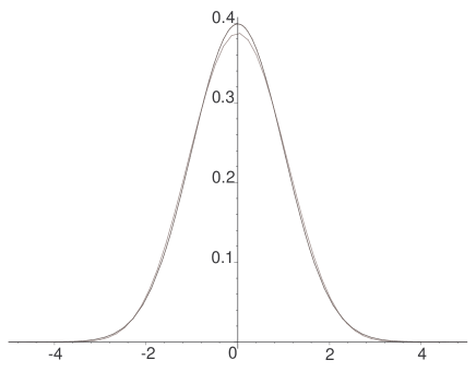
Figure 1.1: The distribution of the coefficients of $\mathscr{D}_{10}$ compared with the normal distribution.

Write the set $\{\bar{1},\bar{2},\ldots,\bar{n}\}$ as $[\bar{n}]$. Let $\mathfrak{S}_{n}^{B}$ denote the hyperoctahedral group of permutations on $[n]\cup[\bar{n}]$, called signed permutations or $B_{n}$-permutations, see Björner and Brenti [5]. Let $\mathscr{D}_{n}^{B}$ denote the set of $B_{n}$-derangements on $[n]$, namely,

$$\mathscr{D}_{n}^{B}=\{\pi=\pi_{1}\pi_{2}\cdots\pi_{n}\in\mathfrak{S}_{n}^{B}\colon\pi_{i}\neq i,\ i=1,2,\ldots,n\}.$$

For example, $\mathscr{D}_{1}^{B}=\{\bar{1}\}$, $\mathscr{D}_{2}^{B}=\left\{\bar{1}\bar{2},21,2\bar{1},\bar{2}1,\bar{2}\bar{1}\right\}$. For $B_{n}$-permutations, Adin and Roichman [3] introduced the notion of the flag major index, or the $\mathrm{fmaj}$ index for short, defined by

$$\mathrm{fmaj}(\pi)=2\mathrm{maj}(\pi)+\mathrm{neg}(\pi),$$

where $\mathrm{maj}(\pi)$ is the major index of $\pi$ with respect to the following order on $[n]\cup[\bar{n}]$:

$$\bar{n}<\cdots<\bar{2}<\bar{1}<1<2<\cdots<n,$$

and $\mathrm{neg}(\pi)$ is the number of $\pi_{i}$’s in $[\bar{n}]$, see also Adin, Brenti and Roichman [2], and Chow and Gessel [8]. For example, the flag major of the $B_{7}$-permutation $35\bar{1}2\bar{6}\bar{7}4$ equals $2\times 11+3=25$. Chow [7] derived the following formula for the $q$-derangement numbers of type $B$:

$$d_{n}^{B}(q)=\sum_{\pi\in\mathscr{D}_{n}^{B}}q^{\mathrm{fmaj}(\pi)}=[2n]_{q}!!\sum_{k=0}^{n}\frac{(-1)^{k}q^{k(k-1)}}{[2k]_{q}!!},$$ (1.2)

where $[2k]_{q}!!=[2k]_{q}[2k-2]_{q}\cdots[2]_{q}$. For $n\leq 4$, the coefficients of the polynomials $d_{n}^{B}(q)$ are given in Table 1.2.

$n\backslash k$	1	2	3	4	5	6	7	8	9	10	11	12	13	14	15	16
1	1
2	1	2	1	1
3	1	3	4	5	5	4	4	2	1
4	1	4	8	13	18	22	26	28	28	25	21	17	11	7	3	1

Table 1.2: The $q$-derangement numbers of type $B$ for $n\leq 4$.

Based on the formula (1.2), we will show that the limiting distribution of the coefficients of $d_{n}^{B}(q)$ is normal. Figure 1.2 is an illustration of the distribution for $n=10$.

Figure 1.2: The distribution of the coefficients of $\mathscr{D}_{10}^{B}$ compared with the normal distribution.

2 The Limiting Distribution of the Coefficients of $d_{n}(q)$

The aim of this section is to show that the limiting distribution of the coefficients of $d_{n}(q)$ is normal. We write

$$f_{n,k}(q)=\begin{cases}1,&\mbox{if }k=n;\\[5.0pt] [n]_{q}[n-1]_{q}\cdots[k+1]_{q},&\mbox{else}.\end{cases}$$

Then we can express $d_{n}(q)$ as

$$d_{n}(q)=\sum_{k=0}^{n}(-1)^{k}q^{k\choose 2}f_{n,k}(q).$$ (2.1)

Let $D_{n}=|\mathscr{D}_{n}|$ be the number of derangements in $\mathscr{D}_{n}$. For example, $D_{1}=0$, $D_{2}=1$, $D_{3}=2$, $D_{4}=9$, $D_{5}=44$.

We will adopt the common notation in asymptotic analysis. If $f(n)$ and $g(n)$ are two functions of $n$, then

• $f(n)=o(g(n))$ means that $\lim_{n\to\infty}f(n)/g(n)=0$;

• $f(n)\sim g(n)$ means that $\lim_{n\to\infty}|f(n)|/|g(n)|=1$.

We now recall some basic facts about the derangement numbers $D_{n}$, see, for example, Stanley [15]. For $n\geq 3$,

$$D_{n} =n!\sum_{k=0}^{n}\frac{(-1)^{k}}{k!}$$ (2.2)

$$=nD_{n-1}+(-1)^{n}$$ (2.3)

$$=(n-1)(D_{n-1}+D_{n-2})$$ (2.4)

$$=\left\lfloor\frac{n!}{e}+\frac{1}{2}\right\rfloor\sim\frac{n!}{e},$$ (2.5)

where the symbol $\lfloor x\rfloor$ denotes the largest integer not exceeding $x$. From (2.3) it immediately follows that

$$\frac{D_{n-1}}{D_{n}}=\frac{1}{n}-\frac{(-1)^{n}}{nD_{n}}\frac{1}{n}+o(1).$$ (2.6)

While it is common to use $\mathrm{maj}(\pi)$ to denote the major index of a permutation $\pi$, there does not seem to be any confusion if we also use $\mathrm{maj}$ to denote the major index of a random derangement on $[n]$. The probability generating function of $\mathrm{maj}$ is clearly $d_{n}(x)/D_{n}$, whereas the moment generating function of $\mathrm{maj}$ is given by

$$M_{n}(x)=\frac{1}{D_{n}}d_{n}\left(e^{x}\right)=\frac{1}{D_{n}}[n]_{e^{x}}!\sum_{k=0}^{n}\frac{(-1)^{k}\,e^{x{k\choose 2}}}{[k]_{e^{x}}!}.$$ (2.7)

Let $E_{n}$, $V_{n}$ and $\sigma_{n}=V_{n}^{1/2}$ denote the expectation, the variance and the standard deviation of $\mathrm{maj}$ respectively. Then the probability generating function $\widetilde{d_{n}}(q)$ of the normalized random variable $(\mathrm{maj}-E_{n})/\sigma_{n}$ equals

$$\widetilde{d_{n}}(q)=\sum_{\pi\in\mathscr{D}_{n}}q^{(\mathrm{maj}(\pi)-E_{n})/\sigma_{n}}=q^{-E_{n}/\sigma_{n}}d_{n}(q^{1/\sigma_{n}}).$$

Thus by the definition (2.7), the moment generating function of $(\mathrm{maj}-E_{n})/\sigma_{n}$ equals

$$\widetilde{M_{n}}(t)=\widetilde{d_{n}}(e^{t})/D_{n}=\exp(-t\,E_{n}/\sigma_{n})M_{n}(t/\sigma_{n}).$$ (2.8)

2.1 The expectation and variance

We now compute the expectation and variance of the major index $\mathrm{maj}$ of a random derangement on $[n]$.

Theorem 2.1

The expectation $E_{n}$ and variance $V_{n}$ of the random variable $\mathrm{maj}$ given by

$$E_{n}=\frac{1}{2}{n\choose 2}\left(1+\frac{D_{n-2}}{D_{n}}\right)=\frac{n^{2}-n+1}{4}+\frac{(-1)^{n}(n-1)}{4D_{n}},$$ (2.9)

and

$$V_{n}=\frac{2n^{3}+3n^{2}-5n-16}{72}+\frac{9n^{3}-4n^{2}-46n+41}{144}\frac{(-1)^{n}}{D_{n}}-\left(\frac{n-1}{4D_{n}}\right)^{2}.$$ (2.10)

Here we give only a sketch of the proof, and detailed steps are omitted.

Proof. The generating function (1.1) implies that

$$E_{n} =\frac{1}{D_{n}}\sum_{\pi\in\mathscr{D}_{n}}\mathrm{maj}(\pi)=\frac{d_{n}^{\prime}(1)}{D_{n}},$$ (2.11)

$$V_{n} =\frac{1}{D_{n}}\sum_{\pi\in\mathscr{D}_{n}}\mathrm{maj}^{2}(\pi)-E_{n}^{2}=\frac{d_{n}^{\prime\prime}(1)}{D_{n}}+E_{n}-E_{n}^{2},$$ (2.12)

where $d^{\prime}_{n}(q)$ and $d^{\prime\prime}_{n}(q)$ are the first and second derivatives of $d_{n}(q)$. From (2.1) and (2.2), we find

$$d_{n}^{\prime}(1)=\sum_{k=0}^{n}(-1)^{k}\left[{k\choose 2}f(1)+f^{\prime}(1)\right]=\frac{1}{2}{n\choose 2}(D_{n}+D_{n-2}).$$

So (2.9) follows from (2.11). Differentiating (2.1) twice yields

$$d_{n}^{\prime\prime}(1)=\sum_{k=0}^{n}(-1)^{k}\left[{k\choose 2}\left({k\choose 2}-1\right)f(1)+2{k\choose 2}f^{\prime}(1)+f^{\prime\prime}(1)\right].$$ (2.13)

The following relations can be easily verified:

$$\sum_{k=0}^{n}(-1)^{k}\left[{k\choose 2}\left({k\choose 2}-1\right)f(1)+2{k\choose 2}f^{\prime}(1)\right]=\frac{3}{2}{n\choose 3}(n+1)D_{n-2},$$

$$\sum_{k=0}^{n}(-1)^{k}f^{\prime\prime}(1)={n\choose 3}\frac{9(n-3)D_{n-4}-32D_{n-3}-18(n+1)D_{n-2}+(9n+13)D_{n}}{24}.$$

Now, using (2.13) and (2.4), we deduce that

$$d_{n}^{\prime\prime}(1)=\frac{1}{72}{n\choose 2}[(n-2)(27n+32)D_{n-2}-(9n+5)D_{n-1}+(n-2)(9n+13)D_{n}].$$

According to (2.12),

$$V_{n} =\frac{n}{144}\left[-(n-1)\left(27n^{2}-13n-23\right)\frac{D_{n-1}}{D_{n}}+\left(9n^{3}+13n^{2}-7n-38\right)\right]$$

$$\quad-\left(\frac{n^{2}}{4}-\frac{n(n-1)}{4}\frac{D_{n-1}}{D_{n}}\right)^{2}.$$

In view of (2.4) and (2.6), we obtain (2.10).  

We note that the formula (2.9) for the expectation of the major index can also be derived by a combinatorial argument, the details are omitted. Based on the estimates (2.5) and (2.6), we derive the following approximations.

Corollary 2.2

We have the following asymptotic estimates:

$$E_{n}=\frac{n^{2}}{4}-\frac{n}{4}+\frac{1}{4}+o(1),\quad\quad V_{n}=\frac{n^{3}}{36}+\frac{n^{2}}{24}-\frac{5n}{72}-\frac{2}{9}+o(1).$$

2.2 The limiting distribution

It is well-known that the moment generating function of a random variable determines its distribution by Curtiss’s theorem (see Curtiss [9] or Sachkov [14]). In particular, if the moment generating function $M_{n}(x)$ of a random variable $\xi_{n}$ has the limit

$$\lim_{n\to\infty}M_{n}(x)=e^{x^{2}/2},$$

then $\xi_{n}$ has as an asymptotically standard normal distribution as $n$ trending to infinity.

We will need Tannery’s theorem (see Tannery [13]) which is essential in the proofs of Lemma 2.4 and Lemma 3.3.

Theorem 2.3 (Tannery’s theorem)

Let $\{v_{k}(n)\}_{k\geq 0}$ be an infinite series satisfying the following two conditions.

• For any fixed $k$, there holds $\lim_{n\to\infty}v_{k}(n)=w_{k}$.

• For any non-negative integer $k$, $|v_{k}(n)|\leq M_{k}$, where $M_{k}$ independent of $n$ and the series $\sum_{k\geq 0}M_{k}$ is convergent.

Then

$$\lim_{n\to\infty}\sum_{k=0}^{m(n)}v_{k}(n)=\sum_{k=0}^{\infty}w_{k},$$

where $m(n)$ is an increasing integer-valued function which trends steadily to infinity as $n$ does.

Lemma 2.4

For any $|x|\leq 1$ and bounded $|t|\leq M$, we have

$$\lim_{n\to\infty}\sum_{k=0}^{n}\frac{x^{k}}{[k]_{e^{-t/\sigma_{n}}}!}=e^{x}.$$ (2.14)

Proof. We apply Tannery’s theorem and set

$$v_{k}(n)=\frac{x^{k}}{[k]_{e^{-t/\sigma_{n}}}!},$$

and $m(n)=n$. Then for any fixed $k$, by Corollary 2.2, it is clear that

$$w_{k}=\lim_{n\to\infty}v_{k}(n)=\frac{x^{k}}{k!}.$$

Note that the right hand side of (2.14) can be expressed as

$$e^{x}=\sum_{k=0}^{\infty}\frac{x^{k}}{k!}=\sum_{k=0}^{\infty}w_{k}.$$

By virtue of Tannery’s theorem, to prove (2.14) it suffices to find an upper bound $M_{k}$ for

$$|v_{k}(n)|=\frac{|x^{k}|}{[k]_{e^{-t/\sigma_{n}}}!},$$

such that $M_{k}$ is independent of $n$ and $\sum_{k=0}^{\infty}M_{k}$ converges. We claim that there exists a constant $c\in(0,1]$ such that $M_{k}=(1+c)^{1-k}$ is the desired upper bound and this bound clearly implies the convergence of $\sum_{k=0}^{\infty}M_{k}=1/c+2+c$.

For $t\leq 0$, we have $e^{-t/\sigma_{n}}\geq 1$ and thus

$$\frac{|x^{k}|}{[k]_{e^{-t/\sigma_{n}}}!}\leq\frac{|x^{k}|}{k!}\leq\frac{1}{k!}\leq\frac{1}{2^{k-1}}\leq M_{k}.$$

For $t\geq 0$, Corollary 2.2 implies that $\sigma_{n}$ has a positive lower bound as $n$ runs over all positive integers and so does $e^{-t/\sigma_{n}}$. Suppose that $e^{-t/\sigma_{n}}\geq c_{t}\in(0,1]$. Since the function $e^{-t/\sigma_{n}}$ is continuous in $t$ and $t$ is bounded, there exists a constant $c\in(0,1]$ independent of $t$ so that $e^{-t/\sigma_{n}}\geq c$ for all $|t|\leq M$. Hence for any $k\geq 1$,

$$\frac{|x^{k}|}{[k]_{e^{-t/\sigma_{n}}}!} =\prod_{j=1}^{k}\frac{|x|}{1+e^{-t/\sigma_{n}}+\cdots+e^{-(j-1)t/\sigma_{n}}}$$

$$\leq\prod_{j=1}^{k}\frac{1}{1+c+\cdots+c^{j-1}}$$

$$\leq\prod_{j=2}^{k}\frac{1}{1+c}=M_{k}.$$

This completes the proof.  

In the computation of the moment generating function of $\mathrm{maj}$, we will need the Bernoulli numbers $B_{k}$ which have the following generating function,

$$\frac{x}{e^{x}-1}=\sum_{k=0}^{\infty}B_{k}\frac{x^{k}}{k!}.$$ (2.15)

The first few Bernoulli numbers are

$$B_{0}=1,\ B_{1}=-1/2,\ B_{2}=1/6,\ B_{3}=0,\ B_{4}=-1/30.$$

Moreover, $B_{2i+1}=0$ for any $i\geq 1$. Alzer [4] establishes sharp bounds for $|B_{2n}|$ leading to the following asymptotic formula (see also [1, pp. 805]) which will be needed in the proof of Lemma 2.5:

$$|B_{2n}|\sim\frac{2\cdotp(2n)!}{(2\pi)^{2n}}.$$ (2.16)

Lemma 2.5

For any bounded $|t|<M$, we have

$$\lim_{n\to\infty}\sum_{i=2}^{\infty}\frac{B_{2i}\,t^{2i}}{(2i)\,(2i)!\,\sigma_{n}^{2i}}\sum_{j=1}^{n}\left(j^{2i}-1\right)=0,$$ (2.17)

where $B_{2i}$ are the Bernoulli numbers.

Proof. Let $\alpha$, $\beta$ and $\gamma$ be three constants such that $\alpha>1$, $\beta>36$, and $0<\gamma<1/2$. Let $N$ be a fixed integer satisfying the following three conditions:

• $n+1<\alpha n$ for any $n>N$;

• $\sigma_{n}^{2}-n^{3}/\beta>0$ for any $n>N$;

• $2\pi N^{\gamma/2}>M\alpha\sqrt{\beta}$.

The existence of such $N$ is obvious. Let $i\geq 2$ and $n>N$. From the inequalities

$$\sum_{j=1}^{n}\left(j^{2i}-1\right)<\int_{1}^{n+1}\left(t^{2i}-1\right)dt=\frac{(n+1)^{2i+1}-1}{2i+1}-n<\frac{(n+1)^{2i+1}}{5}<\frac{(\alpha n)^{2i+1}}{5}$$

and the assumption $\sigma_{n}^{2}>n^{3}/\beta$, we deduce that

$$\frac{1}{\sigma_{n}^{2i}}\sum_{j=1}^{n}\left(j^{2i}-1\right)<\frac{\beta^{i}}{n^{3i}}\frac{(\alpha n)^{2i+1}}{5}=\frac{\alpha}{5}\frac{\left(\alpha\sqrt{\beta}\right)^{2i}}{n^{i-1}}.$$

In light of the inequality

$$\frac{1}{n^{i-1}}=\frac{1}{n^{\gamma i}}\cdot\frac{1}{n^{(1-\gamma)i-1}}<\frac{1}{N^{\gamma i}}\cdot\frac{1}{n^{1-2\gamma}},$$

we see that

$$\lim_{n\to\infty}\sum_{i=2}^{\infty}\frac{B_{2i}\,t^{2i}}{(2i)\,(2i)!\,\sigma_{n}^{2i}}\sum_{j=1}^{n}\left(j^{2i}-1\right)\leq\frac{\alpha}{5}\lim_{n\to\infty}\left(\sum_{i=2}^{\infty}\frac{|B_{2i}|}{(2i)\,(2i)!}\frac{(\alpha\sqrt{\beta})^{2i}}{N^{\gamma i}}t^{2i}\right)n^{2\gamma-1}.$$ (2.18)

By the asymptotic estimate (2.16) for Bernoulli numbers, we see that the radius of convergence (see, for example, Howie [10]) of the series on the right hand of (2.18) equals

$$\lim_{i\to\infty}\left(\frac{|B_{2i}|}{(2i)\,(2i)!}\frac{\left(\alpha\sqrt{\beta}\right)^{2i}}{N^{\gamma i}}\right)^{-\frac{1}{2i}}=\frac{2\pi N^{\gamma/2}}{\alpha\sqrt{\beta}}>M.$$

Since $\lim_{n\to\infty}n^{2\gamma-1}=0$, we conclude that the series in (2.17) is absolutely convergent to zero for $|t|<M$.  

The following lemma gives an expression of the moment generating function of the random variable $\mathrm{maj}$ in term of the Bernoulli numbers. This lemma will be needed in the proof of Theorem 3.6.

Lemma 2.6

The moment generating function of $\mathrm{maj}$ equals

$$M_{n}(x)=\frac{n!}{D_{n}}\exp\left(\frac{n(n-1)x}{4}+\sum_{i=1}^{\infty}\frac{B_{2i}\,x^{2i}}{(2i)\,(2i)!}\sum_{j=1}^{n}\left(j^{2i}-1\right)\right)\sum_{k=0}^{n}\frac{(-1)^{k}}{[k]_{e^{-x}}!}.$$

Proof. By the formula (2.7), we need to express $[n]_{e^{x}}!$ and $e^{x{k\choose 2}}\big{/}[k]_{e^{x}}!$ in terms of Bernoulli numbers. It is known that, see, for example, Mcintosh [12],

$$1-e^{-x}=x\cdotp\exp\left(\sum_{k=1}^{\infty}\frac{B_{n}\,x^{k}}{k\cdotp k!}\right).$$

Thus for any $j\geq 1$,

$$1-e^{xj} =-xj\cdotp\exp\left(\sum_{i=1}^{\infty}\frac{B_{i}(-xj)^{i}}{i\cdotp i!}\right)=-xj\cdotp\exp\left(\frac{xj}{2}+\sum_{i=1}^{\infty}\frac{B_{2i}(xj)^{2i}}{(2i)\,(2i)!}\right),$$

$$[j]_{e^{x}} =\frac{1-e^{xj}}{1-e^{x}}=j\cdotp\exp\left(\frac{x(j-1)}{2}+\sum_{i=1}^{\infty}\frac{B_{2i}\,x^{2i}\left(j^{2i}-1\right)}{(2i)\,(2i)!}\right).$$

Therefore,

$$[n]_{e^{x}}! =\prod_{j=1}^{n}[j]_{e^{x}}=\prod_{j=1}^{n}j\cdotp\exp\left(\frac{x(j-1)}{2}+\sum_{i=1}^{\infty}\frac{B_{2i}\,x^{2i}\left(j^{2i}-1\right)}{(2i)\,(2i)!}\right)$$

$$=n!\cdotp\exp\left(\frac{n(n-1)x}{4}+\sum_{i=1}^{\infty}\frac{B_{2i}\,x^{2i}}{(2i)\,(2i)!}\sum_{j=1}^{n}\left(j^{2i}-1\right)\right).$$ (2.19)

Observe that

$$\frac{e^{x{k\choose 2}}}{[k]_{e^{x}}!}=e^{x{k\choose 2}}\left(\prod_{j=1}^{k}\frac{1-e^{jx}}{1-e^{x}}\right)^{-1}=\prod_{j=1}^{k}\frac{1-e^{x}}{1-e^{jx}}\frac{e^{jx}}{e^{x}}=\frac{1}{[k]_{e^{-x}}!}.$$ (2.20)

Substituting (2.19) and (2.20) into (2.7), we obtain the desired expression.  

Theorem 2.7

Let $\mathrm{maj}$ be the major index of a random derangement on $[n]$. Then the distribution of the random variable

$$\xi_{n}={\mathrm{maj}-E_{n}\over\sigma_{n}}$$

converges to the standard normal distribution as $n\to\infty$.

Proof. By Curtiss’s theorem and (2.8), the normality of the distribution of the standardized random variable $\xi_{n}$ can be justified by the following relation

$$\lim_{n\to\infty}e^{-t\,E_{n}/\sigma_{n}}M_{n}(t/\sigma_{n})=e^{t^{2}/2}.$$

By virtue of Lemma 2.6, the above relation can be restated as

$$\lim_{n\to\infty}\frac{n!}{D_{n}}\exp\left(-\frac{tE_{n}}{\sigma_{n}}+\frac{n(n-1)t}{4\sigma_{n}}+\sum_{i=1}^{\infty}\frac{B_{2i}\,t^{2i}}{(2i)\,(2i)!\sigma_{n}^{2i}}\sum_{j=1}^{n}\left(j^{2i}-1\right)\right)\sum_{k=0}^{n}\frac{(-1)^{k}}{[k]_{e^{-t/\sigma_{n}}}!}=e^{t^{2}/2}.$$

First of all, the estimate (2.5) implies that

$$\lim_{n\to\infty}n!/D_{n}=e.$$ (2.21)

By Corollary 2.2, for bounded $t$ we have

$$\lim_{n\to\infty}\left(\frac{n(n-1)t}{4\sigma_{n}}-\frac{tE_{n}}{\sigma_{n}}\right)=\lim_{n\to\infty}\frac{t}{\sigma_{n}}\left(\frac{n(n-1)}{4}-E_{n}\right)=0,$$ (2.22)

It is easily checked that

$$\lim_{n\to\infty}{1\over\sigma_{n}^{2}}\sum_{j=1}^{n}\left(j^{2}-1\right)=12.$$

In view of Lemma 2.5 and the fact that $B_{2}=1/6$, we have

$$\lim_{n\to\infty}\sum_{i=1}^{\infty}\frac{B_{2i}\,t^{2i}}{(2i)\,(2i)!\sigma_{n}^{2i}}\sum_{j=1}^{n}\left(j^{2i}-1\right)=\lim_{n\to\infty}\frac{B_{2}\,t^{2}}{2\cdot 2!\,\sigma_{n}^{2}}\sum_{j=1}^{n}\left(j^{2}-1\right)=\frac{t^{2}}{2}.$$ (2.23)

Finally, taking $x=-1$ in Lemma 2.4, we get

$$\lim_{n\to\infty}\sum_{k=0}^{n}\frac{(-1)^{k}}{[k]_{e^{-t/\sigma_{n}}}!}=e^{-1}.$$ (2.24)

Combining (2.21), (2.22), (2.23) and (2.24), we complete the proof.  

3 The Limiting Distribution of the Coefficients of $d_{n}^{B}(q)$

In this section, we show that the limiting distribution of the $q$-derangement numbers is normal. Let $D_{n}^{B}$ be the number of $B_{n}$-derangements on $[n]$. The first few values of $D_{n}^{B}$ are

$$D_{1}^{B}=1,\ D_{2}^{B}=5,\ D_{3}^{B}=29,\ D_{4}^{B}=233,\ D_{5}^{B}=2329,\ D_{6}^{B}=27949.$$

For $n\geq 3$, we have

$$D_{n}^{B} =d_{n}^{B}(1)=(2n)!!\sum_{k=0}^{n}\frac{(-1)^{k}}{(2k)!!}$$ (3.1)

$$=2nD_{n-1}^{B}+(-1)^{n}$$ (3.2)

$$=(2n-1)D_{n-1}^{B}+(2n-2)D_{n-2}^{B}$$ (3.3)

$$=\left\lfloor\frac{(2n)!!}{\sqrt{e}}+\frac{1}{2}\right\rfloor\sim\frac{(2n)!!}{\sqrt{e}}.$$ (3.4)

For completeness, we present a proof for (3.4):

$$D_{n}^{B}=(2n)!!\sum_{k=0}^{n}\left(-\frac{1}{2}\right)^{k}\frac{1}{k!}=(2n)!!\left(e^{-1/2}-\sum_{k=n+1}^{\infty}\frac{(-1)^{k}}{(2k)!!}\right).$$

It is easy to see that the absolute value of the remainder

$$r_{n}=\sum_{k=n+1}^{\infty}\frac{(-1)^{k}}{(2k)!!}$$

is not greater than the absolute value of the $(n+1)$-st term of the alternating series, i.e., $1/(2n+2)!!$. This yields

$$D_{n}^{B}=(2n)!!/\sqrt{e}-y_{n},$$

where

$$|y_{n}|=|(2n)!!r_{n}|\leq(2n+2)^{-1}\leq 1/4.$$

Since $D_{n}^{B}$ is an integer, (3.4) is verified.

From (3.2) it follows that

$$\frac{D_{n-1}^{B}}{D_{n}^{B}}=\frac{1}{2n}-\frac{(-1)^{n}}{2nD_{n}^{B}}\frac{1}{2n}+o(1).$$ (3.5)

Let $E_{n}^{B}$, $V_{n}^{B}$ and $\sigma_{n}^{B}=\left(V_{n}^{B}\right)^{1/2}$ denote the expectation, the variance and the standard deviation of $\mathrm{fmaj}$ respectively. We also use $\mathrm{fmaj}$ to denote the fmaj index of a random $B_{n}$-derangements on $[n]$. The probability generating function of $\mathrm{fmaj}$ is

$$\widetilde{d_{n}^{B}}(q)=q^{-E_{n}^{B}/\sigma_{n}^{B}}d_{n}^{B}\left(q^{1/\sigma_{n}^{B}}\right).$$

The moment generating function of $\mathrm{fmaj}$ is given by

$$M_{n}^{B}(x)=\frac{1}{D_{n}^{B}}d_{n}^{B}\left(e^{x}\right)=\sum_{k=0}^{\infty}\left(\frac{1}{D_{n}^{B}}\sum_{\pi\in\mathscr{D}_{n}^{B}}\mathrm{fmaj}(\pi)^{k}\right).$$ (3.6)

The normalized random variable $(\mathrm{fmaj}-E_{n}^{B})/\sigma_{n}^{B}$ equals

$$\widetilde{M_{n}^{B}}(t)=\exp\left(-t\,E_{n}^{B}/\sigma_{n}^{B}\right)M_{n}^{B}\left(t/\sigma_{n}^{B}\right).$$ (3.7)

3.1 The expectation and variance

Let $[x^{i}]f(x)$ to denote the coefficient of $x^{i}$ in the expansion of $f(x)$. Then the expectation and variance of $\mathrm{fmaj}$ can be expressed in terms of the moment generating function $M_{n}^{B}(x)$:

$$E_{n}^{B} =\frac{1}{D_{n}^{B}}\sum_{\pi\in\mathscr{D}_{n}^{B}}\mathrm{fmaj}=[x]M_{n}^{B}(x).$$ (3.8)

$$V_{n}^{B} =\left(\frac{1}{D_{n}^{B}}\sum_{\pi\in\mathscr{D}_{n}^{B}}\mathrm{fmaj}^{2}\right)-\left(E_{n}^{B}\right)^{2}=2\left[x^{2}\right]M_{n}^{B}(x)-\left(E_{n}^{B}\right)^{2}.$$ (3.9)

Let $\left\langle x^{2}\right\rangle f(x)$ to denote the truncated sum of $f(x)$ by keeping the terms up to $x^{2}$. Once $\left\langle x^{2}\right\rangle M_{n}^{B}(x)$ is computed, then the first and the second moments are easily extracted. In this notation, we have

$$\left\langle x^{2}\right\rangle e^{rx}=1+rx+r^{2}x^{2}/2.$$

Moreover,

$$\left\langle x^{2}\right\rangle\sum_{r=0}^{2j-1}e^{rx} =2j+{2j\choose 2}x+\frac{j(2j-1)(4j-1)}{6}x^{2},$$

$$\left\langle x^{2}\right\rangle\prod_{j=k+1}^{n}\sum_{r=0}^{2j-1}e^{rx} =\left\langle x^{2}\right\rangle\prod_{j=k+1}^{n}\left(2j+{2j\choose 2}x+\frac{j(2j-1)(4j-1)}{6}x^{2}\right)$$

$$=\frac{(2n)!!}{(2k)!!}\cdot\left(1+\frac{n^{2}-k^{2}}{2}x+c_{1}x^{2}\right),$$

where

$$c_{1} =\sum_{j=k+1}^{n}\frac{j(2j-1)(4j-1)}{6}\frac{1}{2j}+\sum_{k+1\leq i<j\leq n}{2i\choose 2}{2j\choose 2}\frac{1}{2i}\frac{1}{2j}$$

$$=\frac{(n-k)(9n^{3}+4n^{2}+9kn^{2}+6n-9k^{2}n+4kn-1+6k-9k^{3}+4k^{2})}{72}.$$

By the definition (3.6), we find

$$M_{n}^{B}(x)=\frac{1}{D_{n}^{B}}\sum_{k=0}^{n}(-1)^{k}e^{k(k-1)x}\frac{[2n]_{e^{x}}!!}{[2k]_{e^{x}}!!}=\frac{1}{D_{n}^{B}}\sum_{k=0}^{n}(-1)^{k}e^{k(k-1)x}\prod_{j=k+1}^{n}\sum_{r=0}^{2j-1}e^{rx}.$$

It follows that

$$\left\langle x^{2}\right\rangle M_{n}^{B}(x) =\frac{\left\langle x^{2}\right\rangle}{D_{n}^{B}}\sum_{k=0}^{n}(-1)^{k}\left(1+k(k-1)x+\frac{k^{2}(k-1)^{2}}{2}x^{2}\right)\frac{(2n)!!}{(2k)!!}\left(1+\frac{n^{2}-k^{2}}{2}x+c_{1}x^{2}\right)$$

$$=\frac{1}{D_{n}^{B}}\sum_{k=0}^{n}(-1)^{k}\frac{(2n)!!}{(2k)!!}\left(1+\left(\frac{n^{2}-k^{2}}{2}+k(k-1)\right)x+c_{2}x^{2}\right),$$

where

$$c_{2}=c_{1}+k(k-1)\frac{n^{2}-k^{2}}{2}+\frac{k^{2}(k-1)^{2}}{2}.$$

Let $(k)_{i}=k(k-1)\cdots(k-i+1)$ be the lower factorial. We get

$$c_{2}=\frac{9(k)_{4}+14(k)_{3}+(18n^{2}-27)(k)_{2}-18n^{2}k+(9n^{4}+4n^{3}+6n^{2}-n)}{72}.$$

Combining (3.1), (3.3) and (3.8), we find

$$E_{n}^{B} =[x]M_{n}^{B}(x)=\frac{1}{D_{n}^{B}}\sum_{k=0}^{n}(-1)^{k}\frac{(2n)!!}{(2k)!!}\left(\frac{n^{2}-k^{2}}{2}+k(k-1)\right)$$

$$=\frac{n^{2}}{2}+\frac{n}{4}+\left(-\frac{n^{2}}{2}+\frac{3n}{4}\right)\frac{D_{n-1}^{B}}{D_{n}^{B}}.$$

Now, the variance of $\mathrm{fmaj}$ equals

$$\frac{72D_{n}^{B}}{(2n)!!}[x^{2}]M_{n}^{B}(x) =72\sum_{k=0}^{n}(-1)^{k}\frac{c_{2}}{(2k)!!}$$

$$=\sum_{k=0}^{n}(-1)^{k}\left[\frac{9}{2^{4}(2k-8)!!}+\frac{14}{2^{3}(2k-6)!!}+\frac{18n^{2}-27}{2^{2}(2k-4)!!}\right.$$

$$\left.\quad-\frac{18n^{2}}{2(2k-2)!!}+\frac{9n^{4}+4n^{3}+6n^{2}-n}{(2k)!!}\right].$$

It can be deduced that

$$[x^{2}]M_{n}^{B}(x)=\frac{n(72n^{3}+140n^{2}-22n-101)}{576}-\frac{n(216n^{3}-356n^{2}-186n+127)}{576}\frac{D_{n-1}^{B}}{D_{n}^{B}}.$$

Theorem 3.1

The expectation $E_{n}^{B}$ and variance $V_{n}^{B}$ of $\mathrm{fmaj}$ given by

$$E_{n}^{B}=\frac{n^{2}}{2}+\frac{n}{4}+\left(-\frac{n^{2}}{2}+\frac{3n}{4}\right)\frac{D_{n-1}^{B}}{D_{n}^{B}},$$

and

$$V_{n}^{B}=\frac{n\left(68n^{2}-40n-101\right)}{288}-\frac{n\left(72n^{3}-212n^{2}-78n+127\right)}{288}\frac{D_{n-1}^{B}}{D_{n}^{B}}-\frac{n^{2}(2n-3)^{2}}{16}\left(\frac{D_{n-1}^{B}}{D_{n}^{B}}\right)^{2}.$$

In view of (3.4) and (3.5), we obtain the following estimates.

Corollary 3.2

We have the following asymptotic estimates:

$$E_{n}^{B}=\frac{n^{2}}{2}+\frac{3}{8}+o(1),\quad\quad V_{n}^{B}=\frac{n^{3}}{9}+\frac{n^{2}}{6}-\frac{n}{36}-\frac{13}{36}+o(1).$$

3.2 The limiting distribution

We aim to show that the limiting distribution of $\mathrm{fmaj}$ is normal. The following formula is analogous to Lemma 2.4.

Lemma 3.3

For any real $x$ satisfying $|x|\leq 1$ and bounded $|t|<M$,

$$\lim_{n\to\infty}\sum_{k=0}^{n}\frac{x^{k}}{[2k]_{e^{-t/\sigma_{n}^{B}}}!!\,e^{kt/\sigma_{n}^{B}}}=e^{x/2}.$$

Proof. By virtue of Tannery’s theorem, if suffices to find an upper bound $M_{k}$ for

$$|v_{k}(n)|=\frac{|x^{k}|}{[2k]_{e^{-t/\sigma_{n}^{B}}}!!\,e^{kt/\sigma_{n}^{B}}}$$

such that $M_{k}$ is independent of $n$ and $\sum_{k=0}^{\infty}M_{k}$ converges.

If $t\leq 0$, Corollary 3.2 implies that $\sigma_{n}^{B}$ has a positive lower bound as $n$ runs over all positive integers and so does $e^{t/\sigma_{n}^{B}}$. Suppose that $e^{t/\sigma_{n}^{B}}\geq c_{1}\in(0,1]$ for all $|t|\leq M$, where $c_{1}$ is independent of $t$. Then for any $k\geq 0$,

$$\frac{|x^{k}|}{[2k]_{e^{-t/\sigma_{n}^{B}}}!!\,e^{kt/\sigma_{n}^{B}}} =\prod_{j=1}^{k}\frac{|x|}{\left(1+e^{-t/\sigma_{n}^{B}}+e^{-2t/\sigma_{n}^{B}}+\cdots+e^{-(2j-1)t/\sigma_{n}^{B}}\right)e^{t/\sigma_{n}^{B}}}$$

$$=\prod_{j=1}^{k}\frac{|x|}{\left(e^{t/\sigma_{n}^{B}}+1+e^{-t/\sigma_{n}^{B}}+\cdots+e^{-(2j-2)t/\sigma_{n}^{B}}\right)}$$

$$\leq(1+c_{1})^{-k}.$$

Clearly, $\sum_{k\geq 0}(1+c_{1})^{-k}$ is convergent.

We now assume that $t\geq 0$. Suppose $e^{-t/\sigma_{n}}\geq c_{2}\in(0,1]$ where $c_{2}$ is independent of $t$. Then for any $k\geq 1$,

$$\frac{|x^{k}|}{[2k]_{e^{-t/\sigma_{n}^{B}}}!!\,e^{kt/\sigma_{n}^{B}}} =\prod_{j=1}^{k}\frac{|x|}{\left(1+e^{-t/\sigma_{n}^{B}}+\cdots+e^{-(2j-1)t/\sigma_{n}^{B}}\right)e^{kt/\sigma_{n}^{B}}}$$

$$\leq\prod_{j=1}^{k}\frac{1}{1+c_{2}+\cdots+c_{2}^{2j-1}}\leq(1+c_{2})^{-k}.$$

Similarly, $\sum_{k\geq 0}(1+c_{2})^{-k}$ is convergent.  

The following formula, which is similar to Lemma 2.5, will be crucial in the proof of main theorem of this section.

Lemma 3.4

For any bounded $|t|<M$,

$$\lim_{n\to\infty}\sum_{i=2}^{\infty}\frac{B_{2i}\,t^{2i}}{(2i)\,(2i)!\,\left(\sigma_{n}^{B}\right)^{2i}}\sum_{j=1}^{n}\left((2j)^{2i}-1\right)=0,$$ (3.10)

where $B_{2i}$ are the Bernoulli numbers.

Proof. Let $\alpha$, $\beta$ and $\gamma$ be three constants such that $\alpha>2$, $\beta>9$, and $0<\gamma<1/2$. Let $N$ be a fixed integer satisfying the following three conditions:

• $2n+2<\alpha n$ for any $n>N$;

• $\left(\sigma_{n}^{B}\right)^{2}-n^{3}/\beta>0$ for any $n>N$;

• $2\pi N^{\gamma/2}>M\alpha\sqrt{\beta}$.

The existence of such $N$ is evident. Let $i\geq 2$ and $n>N$. We will show that the series in (3.10) is convergent to zero absolutely. It is easy to derive the following upper bound:

$$\sum_{j=1}^{n}\left((2j)^{2i}-1\right)=2^{2i}\sum_{j=1}^{n}j^{2i}-n<2^{2i}\int_{1}^{n+1}t^{2i}dt$$

$$<\frac{2^{2i}(n+1)^{2i+1}}{2i+1}<\frac{(2n+2)^{2i+1}}{5}<\frac{(\alpha n)^{2i+1}}{5}.$$

The rest of the proof is similar to that of Lemma 2.5.  

Lemma 3.5

The following relation holds:

$$M_{n}^{B}(x)=\frac{(2n)!!}{D_{n}^{B}}\,\exp\left(\frac{xn^{2}}{2}+\sum_{i=1}^{\infty}\frac{B_{2i}\,x^{2i}}{(2i)\,(2i)!}\sum_{j=1}^{n}\left((2j)^{2i}-1\right)\right)\sum_{k=0}^{n}\frac{(-1)^{k}}{[2k]_{e^{-x}}!!\,e^{kx}}.$$

Proof. From (3.6) and (1.2), we have

$$M_{n}^{B}(x)=d_{n}^{B}\left(e^{x}\right)/D_{n}^{B}=\frac{1}{D_{n}^{B}}\,[2n]_{e^{x}}!!\sum_{k=0}^{n}\frac{(-1)^{k}\,e^{xk(k-1)}}{[2k]_{e^{x}}!!}.$$ (3.11)

Moreover,

$$[2n]_{e^{x}}!! =\prod_{j=1}^{n}[2j]_{e^{x}}=\prod_{j=1}^{n}(2j)\cdotp\exp\left(\frac{x(2j-1)}{2}+\sum_{i=1}^{\infty}\frac{B_{2i}\,x^{2i}\left((2j)^{2i}-1\right)}{(2i)\,(2i)!}\right)$$

$$=(2n)!!\cdotp\exp\left(\frac{xn^{2}}{2}+\sum_{i=1}^{\infty}\frac{B_{2i}\,x^{2i}}{(2i)\,(2i)!}\sum_{j=1}^{n}\left((2j)^{2i}-1\right)\right),$$ (3.12)

and

$$\frac{e^{xk^{2}}}{[2k]_{e^{x}}!!}=\prod_{j=1}^{k}\frac{e^{(2j-1)x}}{[2j]_{e^{x}}}=\prod_{j=1}^{k}\frac{e^{2jx}}{e^{x}}\frac{1-e^{x}}{1-e^{2jx}}=\prod_{j=1}^{k}\frac{1-e^{-x}}{1-e^{-2jx}}=\frac{1}{[2k]_{e^{-x}}!!}.$$ (3.13)

Substituting (3.12) and (3.13) into (3.11), we deduce the desired relation.  

Theorem 3.6

Let $\mathrm{fmaj}$ be the flag major index of a random $B_{n}$-derangement. Then the distribution of the random variable

$$\xi_{n}^{B}={\mathrm{fmaj}-E_{n}^{B}\over\sigma_{n}^{B}}$$

converges to the standard normal distribution as $n\to\infty$.

Proof. By Curtiss’s theorem and (3.7), normality of the distribution of $\mathrm{fmaj}$ follows from the identity

$$\lim_{n\to\infty}e^{-t\,E_{n}^{B}/\sigma_{n}^{B}}M_{n}^{B}\left(t/\sigma_{n}^{B}\right)=e^{t^{2}/2}.$$ (3.14)

By Lemma 3.5, the left hand side of (3.14) can be expressed as the limit of the following expression:

$$\frac{(2n)!!}{D_{n}^{B}}\exp\left(-\frac{tE_{n}^{B}}{\sigma_{n}^{B}}+\frac{tn^{2}}{2\sigma_{n}^{B}}+\sum_{i=1}^{\infty}\frac{B_{2i}\,t^{2i}}{(2i)\,(2i)!\left(\sigma_{n}^{B}\right)^{2i}}\sum_{j=1}^{n}\left((2j)^{2i}-1\right)\right)\sum_{k=0}^{n}\frac{(-1)^{k}}{[2k]_{e^{-t/\sigma_{n}^{B}}}!!\,e^{kt/\sigma_{n}^{B}}}.$$

First, the estimate (3.4) implies that

$$\lim_{n\to\infty}(2n)!!/D_{n}^{B}=\sqrt{e}.$$ (3.15)

By Corollary 3.2, for bounded $t$ we have

$$\lim_{n\to\infty}\left(-\frac{tE_{n}^{B}}{\sigma_{n}^{B}}+\frac{tn^{2}}{2\sigma_{n}^{B}}\right)=\lim_{n\to\infty}\frac{t}{\sigma_{n}^{B}}\left(\frac{n^{2}}{2}-E_{n}^{B}\right)=0.$$ (3.16)

It is easy to check that

$$\lim_{n\to\infty}\frac{1}{\left(\sigma_{n}^{B}\right)^{2}}\sum_{j=1}^{n}\left((2j)^{2}-1\right)=12.$$

Based on Lemma 3.4 and the fact that $B_{2}=1/6$, we see that

$$\lim_{n\to\infty}\sum_{i=1}^{\infty}\frac{B_{2i}\,t^{2i}}{(2i)\,(2i)!\left(\sigma_{n}^{B}\right)^{2i}}\sum_{j=1}^{n}\left((2j)^{2i}-1\right)=\lim_{n\to\infty}\frac{B_{2}t^{2}}{2\cdot 2!\,\left(\sigma_{n}^{B}\right)^{2}}\sum_{j=1}^{n}((2j)^{2}-1)=\frac{t^{2}}{2}.$$ (3.17)

Finally, taking $x=-1$ in Lemma 3.3, we get

$$\lim_{n\to\infty}\sum_{k=0}^{n}\frac{(-1)^{k}}{[2k]_{e^{-t/\sigma_{n}^{B}}}!!\,e^{kt/\sigma_{n}^{B}}}=e^{-1/2}.$$ (3.18)

Combining (3.15), (3.16), (3.17) and (3.18), we obtain (3.14). This completes the proof.  

Acknowledgments. This work was supported by the 973 Project, the PCSIRT Project of the Ministry of Education, the Ministry of Science and Technology, and the National Science Foundation of China.

References

- [1] M. Abramowitz and I.A. Stegun, Handbook of Mathematical Functions with Formulas, Graphs, and Mathematical Tables, National Bureau of Standards Applied Mathematics Series 55, 1965.
- [2] R.M. Adin, F. Brenti, and Y. Roichman, Descent numbers and major indices for the hyperoctahedral group, Adv. Appl. Math. 27 (2001), 210–224.
- [3] R.M. Adin and Y. Roichman, The flag major index and group actions on polynomial rings, European J. Combin. 22 (2001), 431–446.
- [4] H. Alzer, Sharp bounds for the Bernoulli numbers, Arch. Math. 74 (2000), 207–211.
- [5] A. Björner and F. Brenti, Combinatorics of Coxeter Groups, Springer, New York, NY. 2005.
- [6] W.Y.C. Chen and D.H. Xu, Labeled partitions and the -Derangement Numbers, SIAM J. Discrete Math., to appear.
- [7] C.-O. Chow, On derangement polynomials of type , Sém. Lothar. Combin. 55 (2006), Article B55b.
- [8] C.-O. Chow and I.M. Gessel, On the descent numbers and major indices for the hyperoctahedral group, Adv. Appl. Math. 38 (2007), 275–301.
- [9] J.H. Curtiss, A note on the theory of moment generating functions, Ann. Math. Statist. 13 (1942), No. 4, 430–433.
- [10] J.M. Howie, Complex Analysis, Springer-Verlag, London, 2003.
- [11] I.M. Gessel and C. Reutenauer, Counting permutations with given cycle structure and descent set, J. Combin. Theory Ser. A 64 (1993), 189–215.
- [12] R.J. Mcintosh, Some asymptotic formulae for -shifted factorials, Ramanujan J. 3 (1999), 205–214.
- [13] J. Tannery, Introduction a la Théorie des Fonctions d’une Variable, 2 Ed., Tome 1, Libraire Scientifique A. Hermann, Paris, 1904.
- [14] V.N. Sachkov, Probabilistic Methods in Combinatorial Analysis, Cambridge University Press, New York, NY, 1997.
- [15] R.P. Stanley, Enumerative Combinatorics 1, 2nd Ed., Cambridge, New York, Cambridge University Press, 1997.
- [16] M. Wachs, On -derangement numbers, Proc. Amer. Math. Soc. 106 (1989), 273–278.