Communication-optimal parallel and sequential QR and LU factorizations: theory and practice

Abstract

We present parallel and sequential dense QR factorization algorithms that are both optimal (up to polylogarithmic factors) in the amount of communication they perform, and just as stable as Householder QR. Our first algorithm, Tall Skinny QR (TSQR), factors $m\times n$ matrices in a one-dimensional (1-D) block cyclic row layout, and is optimized for $m\gg n$. Our second algorithm, CAQR (Communication-Avoiding QR), factors general rectangular matrices distributed in a two-dimensional block cyclic layout. It invokes TSQR for each block column factorization.

The new algorithms are superior in both theory and practice. We have extended known lower bounds on communication for sequential and parallel matrix multiplication to provide latency lower bounds, and show these bounds apply to the LU and QR decompositions. We not only show that our QR algorithms attain these lower bounds (up to polylogarithmic factors), but that existing LAPACK and ScaLAPACK algorithms perform asymptotically more communication. We also point out recent LU algorithms in the literature that attain at least some of these lower bounds.

Both TSQR and CAQR have asymptotically lower latency cost in the parallel case, and asymptotically lower latency and bandwidth costs in the sequential case. In practice, we have implemented parallel TSQR on several machines, with speedups of up to $6.7\times$ on 16 processors of a Pentium III cluster, and up to $4\times$ on 32 processors of a BlueGene/L. We have also implemented sequential TSQR on a laptop for matrices that do not fit in DRAM, so that slow memory is disk. Our out-of-DRAM implementation was as little as $2\times$ slower than the predicted runtime as though DRAM were infinite.

We have also modeled the performance of our parallel CAQR algorithm, yielding predicted speedups over ScaLAPACK’s PDGEQRF of up to $9.7\times$ on an IBM Power5, up to $22.9\times$ on a model Petascale machine, and up to $5.3\times$ on a model of the Grid.

1 Introduction

The large and increasing costs of communication motivate redesigning algorithms to avoid communication whenever possible. Communication matters for both parallel and sequential algorithms. In the parallel case, it refers to messages between processors, which may be sent over a network or via a shared memory. In the sequential case, it refers to data movement between different levels of the memory hierarchy. Many authors have pointed out the exponentially growing gaps between floating-point arithmetic rate, bandwidth, and latency, for many different storage devices and networks on modern high-performance computers (see e.g., Graham et al. [graham2005getting]).

We present parallel and sequential dense QR factorization algorithms that are both optimal (sometimes only up to polylogarithmic factors) in the amount of communication they perform, and just as stable as Householder QR. Some of the algorithms are novel, and some extend earlier work. The first set of algorithms, “Tall Skinny QR” (TSQR), are for matrices with many more rows than columns, and the second set, “Communication-Avoiding QR” (CAQR), are for general rectangular matrices. The algorithms have significantly lower latency cost in the parallel case, and significantly lower latency and bandwidth costs in the sequential case, than existing algorithms in LAPACK and ScaLAPACK. Our algorithms are numerically stable in the same senses as in LAPACK and ScaLAPACK.

The new algorithms are superior in both theory and practice. We have extended known lower bounds on communication for sequential and parallel matrix multiplication (see Hong and Kung [hong1981io] and Irony, Toledo, and Tiskin [irony2004communication]) to QR decomposition, and shown both that the new algorithms attain these lower bounds (sometimes only up to polylogarithmic factors), whereas existing LAPACK and ScaLAPACK algorithms perform asymptotically more communication. (LAPACK costs more in both latency and bandwidth, and ScaLAPACK in latency; it turns out that ScaLAPACK already uses optimal bandwidth.) Operation counts are shown in Tables 1–6, and will be discussed below in more detail.

In practice, we have implemented parallel TSQR on several machines, with significant speedups:

• up to $6.7\times$ on 16 processors of a Pentium III cluster, for a $100,000\times 200$ matrix; and

• up to $4\times$ on 32 processors of a BlueGene/L, for a $1,000,000\times 50$ matrix.

Some of this speedup is enabled by TSQR being able to use a much better local QR decomposition than ScaLAPACK can use, such as the recursive variant by Elmroth and Gustavson (see [elmroth2000applying] and the performance results in Section 12). We have also implemented sequential TSQR on a laptop for matrices that do not fit in DRAM, so that slow memory is disk. This requires a special implementation in order to run at all, since virtual memory does not accommodate matrices of the sizes we tried. By extrapolating runtime from matrices that do fit in DRAM, we can say that our out-of-DRAM implementation was as little as $2\times$ slower than the predicted runtime as though DRAM were infinite.

We have also modeled the performance of our parallel CAQR algorithm (whose actual implementation and measurement is future work), yielding predicted speedups over ScaLAPACK’s PDGEQRF of up to $9.7\times$ on an IBM Power5, up to $22.9\times$ on a model Petascale machine, and up to $5.3\times$ on a model of the Grid. The best speedups occur for the largest number of processors used, and for matrices that do not fill all of memory, since in this case latency costs dominate. In general, when the largest possible matrices are used, computation costs dominate the communication costs and improved communication does not help.

Tables 1–6 summarize our performance models for TSQR, CAQR, and ScaLAPACK’s sequential and parallel QR factorizations. We omit lower order terms. In these tables, we make the optimal choice of matrix layout for each algorithm. In the parallel case, that means choosing the block size $b$ as well as the processor grid dimensions $P_{r}\times P_{c}$ in the 2-D block cyclic layout. (See Sections 13.1 and 15.2 for discussion of how to choose these parameters for parallel CAQR resp. ScaLAPACK.) In case the matrix layout is fixed, Table 16 in Section 13 gives a general performance model of parallel CAQR and PDGEQRF as a function of the block size $b$ (we assume square $b\times b$ blocks) and the processor grid dimensions $P_{r}$ and $P_{c}$. (Table 16 shows that for fixed $b$, $P_{r}$ and $P_{c}$, the number of flops and words transferred roughly match, but the number of messages is about $b$ times lower for CAQR.) In the sequential case, choosing the optimal matrix layout means choosing the dimensions of the matrix block in fast memory so as to minimize runtime with respect to the fast memory size $W$. (See Sections LABEL:SS:CAQR-seq-detailed:opt and LABEL:SS:seqLL:factor for discussion of how to choose these parameters for sequential CAQR resp. (Sca)LAPACK QR.) Equation (LABEL:eq:CAQR:seq:modeltime:P) in Appendix LABEL:SS:CAQR-seq-detailed:factor gives the performance model of sequential CAQR as a function of the dimensions of the matrix block in fast memory (or rather, as a function of the $P_{r}\times P_{c}$ block layout, which uniquely determines the matrix block dimensions).

	TSQR	PDGEQRF	Lower bound
# flops	$\frac{2mn^{2}}{P}+\frac{2}{3}n^{3}\log P$	$\frac{2mn^{2}}{P}-\frac{2n^{3}}{3P}$	$\Theta\left(\frac{mn^{2}}{P}\right)$
# words	$\frac{n^{2}}{2}\log P$	$\frac{n^{2}}{2}\log P$	$\frac{n^{2}}{2}\log P$
# messages	$\mathbf{\log P}$	$\mathbf{2n\log P}$	$\mathbf{\log P}$

Table 1: Performance models of parallel TSQR and ScaLAPACK’s parallel QR factorization PDGEQRF on an $m\times n$ matrix with $P$ processors, along with lower bounds on the number of flops, words, and messages. We assume $m/P\geq n$. Everything (messages, words, and flops) is counted along the critical path. The boldface part of the table highlights TSQR’s improvement over ScaLAPACK.

	Par. CAQR	PDGEQRF	Lower bound
# flops	$\frac{2mn^{2}}{P}+\frac{2n^{3}}{3}$	$\frac{2mn^{2}}{P}+\frac{2n^{3}}{3}$	$\Theta\left(\frac{mn^{2}}{P}\right)$
# words	$\sqrt{\frac{mn^{3}}{P}}\log P-\frac{1}{4}\sqrt{\frac{n^{5}}{mP}}\log\left(\frac{nP}{m}\right)$	$\sqrt{\frac{mn^{3}}{P}}\log P-\frac{1}{4}\sqrt{\frac{n^{5}}{mP}}\log\left(\frac{nP}{m}\right)$	$\Theta\left(\sqrt{\frac{mn^{3}}{P}}\right)$
# messages	$\mathbf{\frac{1}{4}\sqrt{\frac{nP}{m}}\log^{2}\left(\frac{mP}{n}\right)\cdot\log\left(P\sqrt{\frac{mP}{n}}\right)}$	$\mathbf{\frac{n}{4}\log\left(\frac{mP^{5}}{n}\right)\log\left(\frac{mP}{n}\right)}$	$\mathbf{\Theta\left(\sqrt{\frac{nP}{m}}\right)}$

Table 2: Performance models of parallel CAQR and ScaLAPACK’s parallel QR factorization PDGEQRF on a $m\times n$ matrix with $P$ processors, along with lower bounds on the number of flops, words, and messages. The matrix is stored in a 2-D $P_{r}\times P_{c}$ block cyclic layout with square $b\times b$ blocks. We choose $b$, $P_{r}$, and $P_{c}$ optimally and independently for each algorithm. We assume $m\geq n$. Everything (messages, words, and flops) is counted along the critical path. The boldface part of the table highlights CAQR’s improvement over ScaLAPACK.

	Par. CAQR	PDGEQRF	Lower bound
# flops	$\frac{4n^{3}}{3P}$	$\frac{4n^{3}}{3P}$	$\Theta\left(\frac{n^{3}}{P}\right)$
# words	$\frac{3n^{2}}{4\sqrt{P}}\log P$	$\frac{3n^{2}}{4\sqrt{P}}\log P$	$\Theta\left(\frac{n^{2}}{\sqrt{P}}\right)$
# messages	$\mathbf{\frac{3}{8}\sqrt{P}\log^{3}P}$	$\mathbf{\frac{5n}{4}\log^{2}P}$	$\mathbf{\Theta\left(\sqrt{P}\right)}$

Table 3: Performance models of parallel CAQR and ScaLAPACK’s parallel QR factorization PDGEQRF on a square $n\times n$ matrix with $P$ processors, along with lower bounds on the number of flops, words, and messages. The matrix is stored in a 2-D $P_{r}\times P_{c}$ block cyclic layout with square $b\times b$ blocks. We choose $b$, $P_{r}$, and $P_{c}$ optimally and independently for each algorithm. Everything (messages, words, and flops) is counted along the critical path. The boldface part of the table highlights CAQR’s improvement over ScaLAPACK.

	Seq. TSQR	Householder QR	Lower bound
# flops	$2mn^{2}$	$2mn^{2}$	$\Theta(mn^{2})$
# words	$2mn$	$\frac{m^{2}n^{2}}{2W}$	$2mn$
# messages	$\frac{2mn}{\widetilde{W}}$	$\frac{mn^{2}}{2W}$	$\frac{2mn}{W}$

Table 4: Performance models of sequential TSQR and blocked sequential Householder QR (either LAPACK’s in-DRAM DGEQRF or ScaLAPACK’s out-of-DRAM PFDGEQRF) on an $m\times n$ matrix with fast memory size $W$, along with lower bounds on the number of flops, words, and messages. We assume $m\gg n$ and $W\geq 3n^{2}/2$. The boldface part of the table highlights TSQR’s improvement over (Sca)LAPACK. $\widetilde{W}=W-n(n+1)/2$, which is at least about $\frac{2}{3}W$.

	Seq. CAQR	Householder QR	Lower bound
# flops	$2mn^{2}-\frac{2n^{3}}{3}$	$2mn^{2}-\frac{2n^{3}}{3}$	$\Theta(mn^{2})$
# words	$\mathbf{3\frac{mn^{2}}{\sqrt{W}}}$	$\mathbf{\frac{m^{2}n^{2}}{2W}-\frac{mn^{3}}{6W}+\frac{3mn}{2}-\frac{3n^{2}}{4}}$	$\mathbf{\Theta(\frac{mn^{2}}{\sqrt{W}})}$
# messages	$\mathbf{12\frac{mn^{2}}{W^{3/2}}}$	$\mathbf{\frac{mn^{2}}{2W}+\frac{2mn}{W}}$	$\mathbf{\Theta(\frac{mn^{2}}{W^{3/2}})}$

Table 5: Performance models of sequential CAQR and blocked sequential Householder QR (either LAPACK’s in-DRAM DGEQRF or ScaLAPACK’s out-of-DRAM PFDGEQRF) on an $m\times n$ matrix with fast memory size $W$, along with lower bounds on the number of flops, words, and messages. The boldface part of the table highlights CAQR’s improvement over (Sca)LAPACK.

	Seq. CAQR	Householder QR	Lower bound
# flops	$\frac{4n^{3}}{3}$	$\frac{4n^{3}}{3}$	$\Theta(n^{3})$
# words	$\mathbf{3\frac{n^{3}}{\sqrt{W}}}$	$\mathbf{\frac{n^{4}}{3W}+\frac{3n^{2}}{4}}$	$\mathbf{\Theta(\frac{n^{3}}{\sqrt{W}})}$
# messages	$\mathbf{12\frac{n^{3}}{W^{3/2}}}$	$\mathbf{\frac{n^{3}}{2W}}$	$\mathbf{\Theta(\frac{n^{3}}{W^{3/2}})}$

Table 6: Performance models of sequential CAQR and blocked sequential Householder QR (either LAPACK’s in-DRAM DGEQRF or ScaLAPACK’s out-of-DRAM PFDGEQRF) on a square $n\times n$ matrix with fast memory size $W$, along with lower bounds on the number of flops, words, and messages. The boldface part of the table highlights CAQR’s improvement over (Sca)LAPACK.

Here are highlights of the six tables in this section. Tables 1–3 concern parallel algorithms. First, Table 1 compares parallel TSQR and ScaLAPACK’s parallel QR factorization PDGEQRF. TSQR requires fewer messages: $\log P$, which is both optimal, and a factor $2n$ fewer messages than ScaLAPACK. Table 2 compares parallel CAQR and PDGEQRF on a general rectangular matrix. Parallel CAQR needs fewer messages: $\Theta(\sqrt{nP/m})$, which is both optimal (modulo polylogarithmic factors), and a factor $\Theta(\sqrt{mn/P})$ fewer messages than ScaLAPACK. Note that $\sqrt{mn/P}$ is the square root of each processor’s local memory size, up to a small constant factor. Table 3 presents the same comparison for the special case of a square $n\times n$ matrix. There again, parallel CAQR requires fewer messages: $\Theta(\sqrt{P})$, which is both optimal and a factor $\Theta(n/\sqrt{P})$ fewer messages than PDGEQRF. This factor is the square root of the local memory size, up to a small constant factor.

Next, Tables 4–6 concern sequential QR factorization algorithms. Table 4 compares sequential TSQR with sequential blocked Householder QR. This is LAPACK’s QR factorization routine DGEQRF when fast memory is cache and slow memory is DRAM, and it is ScaLAPACK’s out-of-DRAM QR factorization routine PFDGEQRF when fast memory is DRAM and slow memory is disk. Sequential TSQR transfers fewer words between slow and fast memory: $2mn$, which is both optimal and a factor $mn/(4W)$ fewer words than transferred by blocked Householder QR. Note that $mn/W$ is how many times larger the matrix is than the fast memory size $W$. Furthermore, TSQR requires fewer messages: $2mn/\widetilde{W}$, which is close to optimal and $O(n)$ times lower than Householder QR. Table 5 compares sequential CAQR and sequential blocked Householder QR on a general rectangular matrix. Sequential CAQR transfers fewer words between slow and fast memory: $\Theta(mn^{2}/\sqrt{W})$, which is both optimal and a factor $\Theta(m/\sqrt{W})$ fewer words transferred than blocked Householder QR. Note that $m/\sqrt{W}$ is $\sqrt{m^{2}/W}$ which is the square root of how many times larger a square $m\times m$ matrix is than the fast memory size. Sequential CAQR also requires fewer messages: $12mn^{2}/W^{3/2}$, which is optimal. We note that our analysis of CAQR applies for any $W$, whereas our analysis of the algorithms in LAPACK and ScaLAPACK assume that at least 2 columns fit in fast memory, that is $W\geq 2m$; otherwise they may communicate even more. Finally, Table 6 presents the same comparison for the special case of a square $n\times n$ matrix. There again, sequential CAQR transfers fewer words between slow and fast memory: $\Theta(n^{3}/\sqrt{W})$, which is both optimal and a factor $\Theta(n/\sqrt{W})$ fewer words transferred than blocked Householder QR. Sequential CAQR also requires fewer messages: $12n^{3}/W^{3/2}$, which is optimal.

We expect parallel CAQR to outperform ScaLAPACK’s current parallel QR factorization especially well in the strong scaling regime, i.e., when the matrix dimensions are constant and the number of processors $P$ varies. Table 3 shows that the number of floating-point operations for both algorithms scales as $1/P$, and the number of words transferred scales as $n^{2}\log P/\sqrt{P}$. However, for ScaLAPACK, the number of messages is proportional to $n\log^{2}P$, whereas for parallel CAQR, the number of messages is proportional to $\sqrt{P}\log^{3}P$, a factor of $n/\sqrt{P}$ fewer messages. In either case, the number of messages grows with the number of processors and also with the data size, if we assume a limited amount of memory per processor, so reducing communication costs is important to achieving strong scalability.

We have concentrated on the cases of a homogeneous parallel computer and a sequential computer with a two-level memory hierarchy. But real computers are obviously more complicated, combining many levels of parallelism and memory hierarchy, perhaps heterogeneously. So we have shown that our parallel and sequential TSQR designs correspond to the two simplest cases of reduction trees (binary and flat, respectively), and that different choices of reduction trees will let us optimize TSQR for more general architectures.

Now we briefly describe related work and our contributions. The tree-based QR idea itself is not novel (see for example, [buttari2007class, cunha2002new, golub1988parallel, gunter2005parallel, kurzak2008qr, pothen1989distributed, quintana-orti2008scheduling, rabani2001outcore]), but we have a number of optimizations and generalizations:

• Our algorithm can perform almost all its floating-point operations using any fast sequential QR factorization routine. In particular, we can achieve significant speedups by invoking Elmroth and Gustavson’s recursive QR (see [elmroth1998new, elmroth2000applying]).

• We apply TSQR to the parallel factorization of arbitrary rectangular matrices in a two-dimensional block cyclic layout.

• We adapt TSQR to work on general reduction trees. This flexibility lets schedulers overlap communication and computation, and minimize communication for more complicated and realistic computers with multiple levels of parallelism and memory hierarchy (e.g., a system with disk, DRAM, and cache on multiple boards each containing one or more multicore chips of different clock speeds, along with compute accelerator hardware like GPUs).

• We prove optimality for both our parallel and sequential algorithms, with a 1-D layout for TSQR and 2-D block layout for CAQR, i.e., that they minimize bandwidth and latency costs. This assumes $O(n^{3})$ (non-Strassen-like algorithms), and is done in a Big-Oh sense, sometimes modulo polylogarithmic terms.

• We describe special cases in which existing sequential algorithms by Elmroth and Gustavson [elmroth2000applying] and also LAPACK’s DGEQRF attain minimum bandwidth. In particular, with the correct choice of block size, Elmroth’s and Gustavson’s RGEQRF algorithm attains minimum bandwidth and flop count, though not minimum latency.

• We observe that there are alternative LU algorithms in the literature that attain at least some of these communication lower bounds: [grigori2008calu] describes a parallel LU algorithm attaining both bandwidth and latency lower bounds, and [toledo1997locality] describes a sequential LU algorithm that at least attains the bandwidth lower bound.

• We outline how to extend both algorithms and optimality results to certain kinds of hierarchical architectures, either with multiple levels of memory hierarchy, or multiple levels of parallelism (e.g., where each node in a parallel machine consists of other parallel machines, such as multicore).

We note that the $Q$ factor is represented as a tree of smaller $Q$ factors, which differs from the traditional layout. Many previous authors did not explain in detail how to apply a stored TSQR $Q$ factor, quite possibly because this is not needed for solving least squares problems. Adjoining the right-hand side(s) to the matrix $A$, and taking the QR factorization of the result, requires only the $R$ factor. Previous authors discuss this optimization. However, many of our applications require storing and working with the implicit representation of the $Q$ factor. Our performance models show that applying this tree-structured $Q$ has about the same cost as the traditionally represented $Q$.

1.1 Outline

The rest of this report is organized as follows. Section 2 first gives a list of terms and abbreviations. We then begin the discussion of Tall Skinny QR by Section 3, which motivates the algorithm, giving a variety of applications where it is used, beyond as a building block for general QR. Section 4 introduces the TSQR algorithm and shows how the parallel and sequential versions correspond to different reduction or all-reduction trees. After that, Section 5 illustrates how TSQR is actually a reduction, introduces corresponding terminology, and discusses some design choices. Section 6 shows how the local QR decompositions in TSQR can be further optimized, including ways that current ScaLAPACK cannot exploit. We also explain how to apply the $Q$ factor from TSQR efficiently, which is needed both for general QR and other applications. Section 7 explains about our parallel and sequential machine models, and what parameters we use to describe them. Next, Sections 9 and 10 describe other ”tall skinny QR” algorithms, such as CholeskyQR and Gram-Schmidt, and compare their cost (Section 9) and numerical stability (Section 10) to that of TSQR. These sections show that TSQR is the only algorithm that simultaneously minimizes communication and is numerically stable. Section 11 describes the platforms used for testing TSQR, and Section 12 concludes the discussion of TSQR proper by describing the TSQR performance results.

Our discussion of CAQR presents both the parallel and the sequential CAQR algorithms for the QR factorization of general rectangular matrices. Section 13 describes the parallel CAQR algorithm and constructs a performance model. Section 14 does the same for sequential CAQR. Subsection 14.1 analyzes other sequential QR algorithms including those of Elmroth and Gustavson. Next, Section 15 compares the performance of parallel CAQR and ScaLAPACK’s PDGEQRF, showing CAQR to be superior, for the same choices of block sizes and data layout parameters, as well as when these parameters are chosen optimally and independently for CAQR and PDGEQRF. After that, Section 16 presents performance predictions comparing CAQR to PDGEQRF. Future work includes actual implementation and measurements.

The next two sections in the body of the text concern theoretical results about CAQR and other parallel and sequential QR factorizations. Section 17 describes how to extend known lower bounds on communication for matrix multiplication to QR, and shows that these are attained (modulo polylogarithmic factors) by TSQR and CAQR. Section LABEL:S:limits-to-par reviews known lower bounds on parallelism for QR, using a PRAM model of parallel computation.

The final section, Section LABEL:S:hierarchies briefly outlines how to extend the algorithms and optimality results to hierarchical architectures, either with several levels of memory hierarchy, or several levels of parallelism.

The Appendices provide details of operation counts and other results summarized in previous sections. Appendix LABEL:S:localQR-flops presents flop counts for optimizations of local QR decompositions described in Section 6. Appendices LABEL:S:TSQR-seq-detailed, LABEL:S:CAQR-seq-detailed, LABEL:S:TSQR-par-detailed, and LABEL:S:CAQR-par-detailed give details of performance models for sequential TSQR, sequential CAQR, parallel TSQR and parallel CAQR, respectively. Appendix LABEL:S:PFDGEQRF models sequential QR based on ScaLAPACK’s out-of-DRAM routine PFDGEQRF. Finally, Appendix LABEL:S:CommLowerBoundsFromCalculus proves communication lower bounds needed in Section 17.

1.2 Future work

Implementations of sequential and parallel CAQR are currently underway. Optimization of the TSQR reduction tree for more general, practical architectures (such as multicore, multisocket, or GPUs) is future work, as well as optimization of the rest of CAQR to the most general architectures, with proofs of optimality.

It is natural to ask to how much of dense linear algebra one can extend the results of this paper, that is finding algorithms that attain communication lower bounds. In the case of parallel LU with pivoting, refer to the technical report by Grigori, Demmel, and Xiang [grigori2008calu], and in the case of sequential LU, refer to the paper by Toledo [toledo1997locality] (at least for minimizing bandwidth). More broadly, we hope to extend the results of this paper to the rest of linear algebra, including two-sided factorizations (such as reduction to symmetric tridiagonal, bidiagonal, or (generalized) upper Hessenberg forms). Once a matrix is symmetric tridiagonal (or bidiagonal) and so takes little memory, fast algorithms for the eigenproblem (or SVD) are available. Most challenging is likely to be find eigenvalues of a matrix in upper Hessenberg form (or of a matrix pencil).

2 List of terms and abbreviations

alpha-beta model

A simple model for communication time, involving a latency parameter $\alpha$ and an inverse bandwidth parameter $\beta$: the time to transfer a single message containing $n$ words is $\alpha+\beta n$.

CAQR

Communication-Avoiding QR – a parallel and/or explicitly swapping QR factorization algorithm, intended for input matrices of general shape. Invokes TSQR for panel factorizations.

CholeskyQR

A fast but numerically unstable QR factorization algorithm for tall and skinny matrices, based on the Cholesky factorization of $A^{T}A$.

DGEQRF

LAPACK QR factorization routine for general dense matrices of double-precision floating-point numbers. May or may not exploit shared-memory parallelism via a multithreaded BLAS implementation.

GPU

Graphics processing unit.

Explicitly swapping

Refers to algorithms explicitly written to save space in one level of the memory hierarchy (“fast memory”) by using the next level (“slow memory”) as swap space. Explicitly swapping algorithms can solve problems too large to fit in fast memory. Special cases include out-of-DRAM (a.k.a. out-of-core), out-of-cache (which is a performance optimization that manages cache space explicitly in the algorithm), and algorithms written for processors with non-cache-coherent local scratch memory and global DRAM (such as Cell).

Flash drive

A persistent storage device that uses nonvolatile flash memory, rather than the spinning magnetic disks used in hard drives. These are increasingly being used as replacements for traditional hard disks for certain applications. Flash drives are a specific kind of solid-state drive (SSD), which uses solid-state (not liquid, gas, or plasma) electronics with no moving parts to store data.

Local store

A user-managed storage area which functions like a cache (in that it is smaller and faster than main memory), but has no hardware support for cache coherency.

Out-of-cache

Refers to algorithms explicitly written to save space in cache (or local store), by using the next larger level of cache (or local store), or main memory (DRAM), as swap space.

Out-of-DRAM

Refers to algorithms explicitly written to save space in main memory (DRAM), by using disk as swap space. (“Core” used to mean “main memory,” as main memories were once constructed of many small solenoid cores.) See explicitly swapping.

PDGEQRF

ScaLAPACK parallel QR factorization routine for general dense matrices of double-precision floating-point numbers.

PFDGEQRF

ScaLAPACK parallel out-of-core QR factorization routine for general dense matrices of double-precision floating-point numbers.

TSQR

Tall Skinny QR – our reduction-based QR factorization algorithm, intended for “tall and skinny” input matrices (i.e., those with many more rows than columns).

3 Motivation for TSQR

3.1 Block iterative methods

Block iterative methods frequently compute the QR factorization of a tall and skinny dense matrix. This includes algorithms for solving linear systems $Ax=B$ with multiple right-hand sides (such as variants of GMRES, QMR, or CG [vital:phdthesis:90, Freund:1997:BQA, oleary:80]), as well as block iterative eigensolvers (for a summary of such methods, see [templatesEigenBai, templatesEigenLehoucq]). Many of these methods have widely used implementations, on which a large community of scientists and engineers depends for their computational tasks. Examples include TRLAN (Thick Restart Lanczos), BLZPACK (Block Lanczos), Anasazi (various block methods), and PRIMME (block Jacobi-Davidson methods) [TRLANwebpage, BLZPACKwebpage, BLOPEXwebpage, irbleigs, TRILINOSwebpage, PRIMMEwebpage]. Eigenvalue computation is particularly sensitive to the accuracy of the orthogonalization; two recent papers suggest that large-scale eigenvalue applications require a stable QR factorization [lehoucqORTH, andrewORTH].

3.2 $s$-step Krylov methods

Recent research has reawakened an interest in alternate formulations of Krylov subspace methods, called $s$-step Krylov methods, in which some number $s$ steps of the algorithm are performed all at once, in order to reduce communication. Demmel et al. review the existing literature and discuss new advances in this area [demmel2008comm]. Such a method begins with an $n\times n$ matrix $A$ and a starting vector $v$, and generates some basis for the Krylov subspace $\operatorname{span}\{v$, $Av$, $A^{2}v$, $\dots$, $A^{s}v\}$, using a small number of communication steps that is independent of $s$. Then, a QR factorization is used to orthogonalize the basis vectors.

The goal of combining $s$ steps into one is to leverage existing basis generation algorithms that reduce the number of messages and/or the volume of communication between different levels of the memory hierarchy and/or different processors. These algorithms make the resulting number of messages independent of $s$, rather than growing with $s$ (as in standard Krylov methods). However, this means that the QR factorization is now the communications bottleneck, at least in the parallel case: the current PDGEQRF algorithm in ScaLAPACK takes $2s\log_{2}P$ messages (in which $P$ is the number of processors), compared to $\log_{2}P$ messages for TSQR. Numerical stability considerations limit $s$, so that it is essentially a constant with respect to the matrix size $m$. Furthermore, a stable QR factorization is necessary in order to restrict the loss of stability caused by generating $s$ steps of the basis without intermediate orthogonalization. This is an ideal application for TSQR, and in fact inspired its (re-)discovery.

3.3 Panel factorization in general QR

Householder QR decompositions of tall and skinny matrices also comprise the panel factorization step for typical QR factorizations of matrices in a more general, two-dimensional layout. This includes the current parallel QR factorization routine PDGEQRF in ScaLAPACK, as well as ScaLAPACK’s out-of-DRAM QR factorization PFDGEQRF. Both algorithms use a standard column-based Householder QR for the panel factorizations, but in the parallel case this is a latency bottleneck, and in the out-of-DRAM case it is a bandwidth bottleneck. Replacing the existing panel factorization with TSQR would reduce this cost by a factor equal to the number of columns in a panel, thus removing the bottleneck. TSQR requires more floating-point operations, though some of this computation can be overlapped with communication. Section 13 will discuss the advantages of this approach in detail.

4 TSQR matrix algebra

In this section, we illustrate the insight behind the TSQR algorithm. TSQR uses a reduction-like operation to compute the QR factorization of an $m\times n$ matrix $A$, stored in a 1-D block row layout. We begin with parallel TSQR on a binary tree of four processors ($P=4$), and later show sequential TSQR on a linear tree with four blocks.

4.1 Parallel TSQR on a binary tree

Figure 1: Execution of the parallel TSQR factorization on a binary tree of four processors. The gray boxes indicate where local QR factorizations take place. The $Q$ and $R$ factors each have two subscripts: the first is the sequence number within that stage, and the second is the stage number.

The basic idea of using a reduction on a binary tree to compute a tall skinny QR factorization has been rediscovered more than once (see e.g., [cunha2002new, pothen1989distributed]). (TSQR was also suggested by Golub et al. [golub1988parallel], but they did not reduce the number of messages from $n\log P$ to $\log P$.) We repeat it here in order to show its generalization to a whole space of algorithms. First, we decompose the $m\times n$ matrix $A$ into four $m/4\times n$ block rows:

$$A=\begin{pmatrix}A_{0}\\ A_{1}\\ A_{2}\\ A_{3}\\ \end{pmatrix}.$$

Then, we independently compute the QR factorization of each block row:

$$\begin{pmatrix}A_{0}\\ A_{1}\\ A_{2}\\ A_{3}\\ \end{pmatrix}=\begin{pmatrix}Q_{00}R_{00}\\ Q_{10}R_{10}\\ Q_{20}R_{20}\\ Q_{30}R_{30}\\ \end{pmatrix}.$$

This is “stage 0” of the computation, hence the second subscript 0 of the $Q$ and $R$ factors. The first subscript indicates the block index at that stage. (Abstractly, we use the Fortran convention that the first index changes “more frequently” than the second index.) Stage 0 operates on the $P=4$ leaves of the tree. We can write this decomposition instead as a block diagonal orthogonal matrix times a column of blocks:

$$A=\begin{pmatrix}Q_{00}R_{00}\\ Q_{10}R_{10}\\ Q_{20}R_{20}\\ Q_{30}R_{30}\\ \end{pmatrix}=\left(\begin{array}[]{c | c | c | c}Q_{00}&&&\\ \hline\cr&Q_{10}&&\\ \hline\cr&&Q_{20}&\\ \hline\cr&&&Q_{30}\\ \end{array}\right)\cdot\begin{pmatrix}R_{00}\\ \hline\cr R_{10}\\ \hline\cr R_{20}\\ \hline\cr R_{30}\\ \end{pmatrix},$$

although we do not have to store it this way. After this stage 0, there are $P=4$ of the $R$ factors. We group them into successive pairs $R_{i,0}$ and $R_{i+1,0}$, and do the QR factorizations of grouped pairs in parallel:

$$\begin{pmatrix}R_{00}\\ R_{10}\\ \hline\cr R_{20}\\ R_{30}\\ \end{pmatrix}=\begin{pmatrix}\begin{pmatrix}R_{00}\\ R_{10}\\ \end{pmatrix}\\ \hline\cr\begin{pmatrix}R_{20}\\ R_{30}\\ \end{pmatrix}\end{pmatrix}=\begin{pmatrix}Q_{01}R_{01}\\ \hline\cr Q_{11}R_{11}\\ \end{pmatrix}.$$

As before, we can rewrite the last term as a block diagonal orthogonal matrix times a column of blocks:

$$\begin{pmatrix}Q_{01}R_{01}\\ \hline\cr Q_{11}R_{11}\\ \end{pmatrix}=\left(\begin{array}[]{c | c}Q_{01}&\\ \hline\cr&Q_{11}\\ \end{array}\right)\cdot\begin{pmatrix}R_{01}\\ \hline\cr R_{11}\\ \end{pmatrix}.$$

This is stage 1, as the second subscript of the $Q$ and $R$ factors indicates. We iteratively perform stages until there is only one $R$ factor left, which is the root of the tree:

$$\begin{pmatrix}R_{01}\\ R_{11}\\ \end{pmatrix}=Q_{02}R_{02}.$$

Equation (1) shows the whole factorization:

$$A=\begin{pmatrix}A_{0}\\ A_{1}\\ A_{2}\\ A_{3}\\ \end{pmatrix}=\left(\begin{array}[]{c | c | c | c}Q_{00}&&&\\ \hline\cr&Q_{10}&&\\ \hline\cr&&Q_{20}&\\ \hline\cr&&&Q_{30}\\ \end{array}\right)\cdot\left(\begin{array}[]{c | c}Q_{01}&\\ \hline\cr&Q_{11}\\ \end{array}\right)\cdot Q_{02}\cdot R_{02},$$ (1)

in which the product of the first three matrices has orthogonal columns, since each of these three matrices does. Note the binary tree structure in the nested pairs of $R$ factors.

Figure 1 illustrates the binary tree on which the above factorization executes. Gray boxes highlight where local QR factorizations take place. By “local,” we refer to a factorization performed by any one processor at one node of the tree; it may involve one or more than one block row. If we were to compute all the above $Q$ factors explicitly as square matrices, each of the $Q_{i0}$ would be $m/P\times m/P$, and $Q_{ij}$ for $j>0$ would be $2n\times 2n$. The final $R$ factor would be upper triangular and $m\times n$, with $m-n$ rows of zeros. In a “thin QR” factorization, in which the final $Q$ factor has the same dimensions as $A$, the final $R$ factor would be upper triangular and $n\times n$. In practice, we prefer to store all the local $Q$ factors implicitly until the factorization is complete. In that case, the implicit representation of $Q_{i0}$ fits in an $m/P\times n$ lower triangular matrix, and the implicit representation of $Q_{ij}$ (for $j>0$) fits in an $n\times n$ lower triangular matrix (due to optimizations that will be discussed in Section 6).

Note that the maximum per-processor memory requirement is $\max\{mn/P,n^{2}+O(n)\}$, since any one processor need only factor two $n\times n$ upper triangular matrices at once, or a single $m/P\times n$ matrix.

4.2 Sequential TSQR on a flat tree

Figure 2: Execution of the sequential TSQR factorization on a flat tree with four submatrices. The gray boxes indicate where local QR factorizations take place The $Q$ and $R$ factors each have two subscripts: the first is the sequence number for that stage, and the second is the stage number.

Sequential TSQR uses a similar factorization process, but with a “flat tree” (a linear chain). It may also handle the leaf nodes of the tree slightly differently, as we will show below. Again, the basic idea is not new; see e.g., [buttari2007class, buttari2007parallel, gunter2005parallel, kurzak2008qr, quintana-orti2008scheduling, rabani2001outcore]. (Some authors (e.g., [buttari2007class, kurzak2008qr, quintana-orti2008scheduling]) refer to sequential TSQR as “tiled QR.” We use the phrase “sequential TSQR” because both our parallel and sequential algorithms could be said to use tiles.) In particular, Gunter and van de Geijn develop a parallel out-of-DRAM QR factorization algorithm that uses a flat tree for the panel factorizations [gunter2005parallel]. Buttari et al. suggest using a QR factorization of this type to improve performance of parallel QR on commodity multicore processors [buttari2007class]. Quintana-Orti et al. develop two variations on block QR factorization algorithms, and use them with a dynamic task scheduling system to parallelize the QR factorization on shared-memory machines [quintana-orti2008scheduling]. Kurzak and Dongarra use similar algorithms, but with static task scheduling, to parallelize the QR factorization on Cell processors [kurzak2008qr]. The reason these authors use what we call sequential TSQR in a parallel context …

We will show that the basic idea of sequential TSQR fits into the same general framework as the parallel QR decomposition illustrated above, and also how this generalization expands the tuning space of QR factorization algorithms. In addition, we will develop detailed performance models of sequential TSQR and the current sequential QR factorization implemented in LAPACK.

We start with the same block row decomposition as with parallel TSQR above:

$$A=\begin{pmatrix}A_{0}\\ A_{1}\\ A_{2}\\ A_{3}\\ \end{pmatrix}$$

but begin with a QR factorization of $A_{0}$, rather than of all the block rows:

$$\begin{pmatrix}A_{0}\\ A_{1}\\ A_{2}\\ A_{3}\\ \end{pmatrix}=\begin{pmatrix}Q_{00}R_{00}\\ A_{1}\\ A_{2}\\ A_{3}\\ \end{pmatrix}.$$

This is “stage 0” of the computation, hence the second subscript 0 of the $Q$ and $R$ factor. We retain the first subscript for generality, though in this example it is always zero. We can write this decomposition instead as a block diagonal matrix times a column of blocks:

$$\begin{pmatrix}Q_{00}R_{00}\\ A_{1}\\ A_{2}\\ A_{3}\\ \end{pmatrix}=\left(\begin{array}[]{c | c | c | c}Q_{00}&&&\\ \hline\cr&I&&\\ \hline\cr&&I&\\ \hline\cr&&&I\\ \end{array}\right)\cdot\begin{pmatrix}R_{00}\\ \hline\cr A_{1}\\ \hline\cr A_{2}\\ \hline\cr A_{3}\\ \end{pmatrix}.$$

We then combine $R_{00}$ and $A_{1}$ using a QR factorization:

$$\begin{pmatrix}R_{00}\\ A_{1}\\ A_{2}\\ A_{3}\\ \end{pmatrix}=\begin{pmatrix}R_{00}\\ A_{1}\\ \hline\cr A_{2}\\ A_{3}\\ \end{pmatrix}=\begin{pmatrix}Q_{01}R_{01}\\ \hline\cr A_{2}\\ A_{3}\\ \end{pmatrix}$$

This can be rewritten as a block diagonal matrix times a column of blocks:

$$\begin{pmatrix}Q_{01}R_{01}\\ \hline\cr A_{2}\\ A_{3}\\ \end{pmatrix}=\left(\begin{array}[]{c | c | c}Q_{01}&&\\ \hline\cr&I&\\ \hline\cr&&I\\ \end{array}\right)\cdot\begin{pmatrix}R_{01}\\ \hline\cr A_{2}\\ \hline\cr A_{3}\\ \end{pmatrix}.$$

We continue this process until we run out of $A_{i}$ factors. The resulting factorization has the following structure:

$$\begin{pmatrix}A_{0}\\ A_{1}\\ A_{2}\\ A_{3}\\ \end{pmatrix}=\left(\begin{array}[]{c | c | c | c}Q_{00}&&&\\ \hline\cr&I&&\\ \hline\cr&&I&\\ \hline\cr&&&I\\ \end{array}\right)\cdot\left(\begin{array}[]{c | c | c}Q_{01}&&\\ \hline\cr&I&\\ \hline\cr&&I\\ \end{array}\right)\cdot\left(\begin{array}[]{c | c | c}I&&\\ \hline\cr&Q_{02}&\\ \hline\cr&&I\\ \end{array}\right)\cdot\left(\begin{array}[]{c | c | c}I&&\\ \hline\cr&I&\\ \hline\cr&&Q_{03}\\ \end{array}\right)R_{30}.$$ (2)

Here, the $A_{i}$ blocks are $m/P\times n$. If we were to compute all the above $Q$ factors explicitly as square matrices, then $Q_{00}$ would be $m/P\times m/P$ and $Q_{0j}$ for $j>0$ would be $2m/P\times 2m/P$. The above $I$ factors would be $m/P\times m/P$. The final $R$ factor, as in the parallel case, would be upper triangular and $m\times n$, with $m-n$ rows of zeros. In a “thin QR” factorization, in which the final $Q$ factor has the same dimensions as $A$, the final $R$ factor would be upper triangular and $n\times n$. In practice, we prefer to store all the local $Q$ factors implicitly until the factorization is complete. In that case, the implicit representation of $Q_{00}$ fits in an $m/P\times n$ lower triangular matrix, and the implicit representation of $Q_{0j}$ (for $j>0$) fits in an $m/P\times n$ lower triangular matrix as well (due to optimizations that will be discussed in Section 6).

Figure 2 illustrates the flat tree on which the above factorization executes. Gray boxes highlight where “local” QR factorizations take place.

The sequential algorithm differs from the parallel one in that it does not factor the individual blocks of the input matrix $A$, excepting $A_{0}$. This is because in the sequential case, the input matrix has not yet been loaded into working memory. In the fully parallel case, each block of $A$ resides in some processor’s working memory. It then pays to factor all the blocks before combining them, as this reduces the volume of communication (only the triangular $R$ factors need to be exchanged) and reduces the amount of arithmetic performed at the next level of the tree. In contrast, the sequential algorithm never writes out the intermediate $R$ factors, so it does not need to convert the individual $A_{i}$ into upper triangular factors. Factoring each $A_{i}$ separately would require writing out an additional $Q$ factor for each block of $A$. It would also add another level to the tree, corresponding to the first block $A_{0}$.

Note that the maximum per-processor memory requirement is $mn/P+n^{2}/2+O(n)$, since only an $m/P\times n$ block and an $n\times n$ upper triangular block reside in fast memory at one time. We could save some fast memory by factoring each $A_{i}$ block separately before combining it with the next block’s $R$ factor, as long as each block’s $Q$ and $R$ factors are written back to slow memory before the next block is loaded. One would then only need to fit no more than two $n\times n$ upper triangular factors in fast memory at once. However, this would result in more writes, as each $R$ factor (except the last) would need to be written to slow memory and read back into fact memory, rather than just left in fast memory for the next step.

In both the parallel and sequential algorithms, a vector or matrix is multiplied by $Q$ or $Q^{T}$ by using the implicit representation of the $Q$ factor, as shown in Equation (1) for the parallel case, and Equation (2) for the sequential case. This is analogous to using the Householder vectors computed by Householder QR as an implicit representation of the $Q$ factor.

4.3 TSQR on general trees

Figure 3: Execution of a hybrid parallel / out-of-core TSQR factorization. The matrix has 16 blocks, and four processors can execute local QR factorizations simultaneously. The gray boxes indicate where local QR factorizations take place. We number the blocks of the input matrix $A$ in hexadecimal to save space (which means that the subscript letter A is the number $10_{10}$, but the non-subscript letter $A$ is a matrix block). The $Q$ and $R$ factors each have two subscripts: the first is the sequence number for that stage, and the second is the stage number.

The above two algorithms are extreme points in a large set of possible QR factorization methods, parametrized by the tree structure. Our version of TSQR is novel because it works on any tree. In general, the optimal tree may depend on both the architecture and the matrix dimensions. This is because TSQR is a reduction (as we will discuss further in Section 5). Trees of types other than binary often result in better reduction performance, depending on the architecture (see e.g., [nishtala2008performance]). Throughout this paper, we discuss two examples – the binary tree and the flat tree – as easy extremes for illustration. We will show that the binary tree minimizes the number of stages and messages in the parallel case, and that the flat tree minimizes the number and volume of input matrix reads and writes in the sequential case. Section 5 shows how to perform TSQR on any tree. Methods for finding the best tree in the case of TSQR are future work. Nevertheless, we can identify two regimes in which a “nonstandard” tree could improve performance significantly: parallel memory-limited CPUs, and large distributed-memory supercomputers.

The advent of desktop and even laptop multicore processors suggests a revival of parallel out-of-DRAM algorithms, for solving cluster-sized problems while saving power and avoiding the hassle of debugging on a cluster. TSQR could execute efficiently on a parallel memory-limited device if a sequential flat tree were used to bring blocks into memory, and a parallel tree (with a structure that reflects the multicore memory hierarchy) were used to factor the blocks. Figure 3 shows an example with 16 blocks executing on four processors, in which the factorizations are pipelined for maximum utilization of the processors. The algorithm itself needs no modification, since the tree structure itself encodes the pipelining. This is, we believe, a novel extension of the parallel out-of-core QR factorization of Gunter et al. [gunter2005parallel].

TSQR’s choice of tree shape can also be optimized for modern supercomputers. A tree with different branching factors at different levels could naturally accommodate the heterogeneous communication network of a cluster of multicores. The subtrees at the lowest level may have the same branching factor as the number of cores per node (or per socket, for a multisocket shared-memory architecture).

Note that the maximum per-processor memory requirement of all TSQR variations is bounded above by

$$\frac{qn(n+1)}{2}+\frac{mn}{P},$$

in which $q$ is the maximum branching factor in the tree.

5 TSQR as a reduction

Section 4 explained the algebra of the TSQR factorization. It outlined how to reorganize the parallel QR factorization as a tree-structured computation, in which groups of neighboring processors combine their $R$ factors, perform (possibly redundant) QR factorizations, and continue the process by communicating their $R$ factors to the next set of neighbors. Sequential TSQR works in a similar way, except that communication consists of moving matrix factors between slow and fast memory. This tree structure uses the same pattern of communication found in a reduction or all-reduction. Thus, effective optimization of TSQR requires understanding these operations.

5.1 Reductions and all-reductions

Reductions and all-reductions are operations that take a collection as input, and combine the collection using some (ideally) associative function into a single item. The result is a function of all the items in the input. Usually, one speaks of (all-) reductions in the parallel case, where ownership of the input collection is distributed across some number $P$ of processors. A reduction leaves the final result on exactly one of the $P$ processors; an all-reduction leaves a copy of the final result on all the processors. See, for example, [gropp1999using].

In the sequential case, there is an analogous operation. Imagine that there are $P$ “virtual processors.” To each one is assigned a certain amount of fast memory. Virtual processors communicate by sending messages via slow memory, just as the “real processors” in the parallel case communicate via the (relatively slow) network. Each virtual processor owns a particular subset of the input data, just as each real processor does in a parallel implementation. A virtual processor can read any other virtual processor’s subset by reading from slow memory (this is a “receive”). It can also write some data to slow memory (a “send”), for another virtual processor to read. We can run programs for this virtual parallel machine on an actual machine with only one processor and its associated fast memory by scheduling the virtual processors’ tasks on the real processor(s) in a way that respects task dependencies. Note that all-reductions and reductions produce the same result when there is only one actual processor, because if the final result ends up in fast memory on any of the virtual processors, it is also in fast memory on the one actual processor.

The “virtual processors” argument may also have practical use when implementing (all-) reductions on clusters of SMPs or vector processors, multicore out-of-core, or some other combination consisting of tightly-coupled parallel units with slow communication links between the units. A good mapping of virtual processors to real processors, along with the right scheduling of the “virtual” algorithm on the real machine, can exploit multiple levels of parallelism and the memory hierarchy.

5.2 (All-) reduction trees

Reductions and all-reductions are performed on directed trees. In a reduction, each node represents a processor, and each edge a message passed from one processor to another. All-reductions have two different implementation strategies:

• “Reduce-broadcast”: Perform a standard reduction to one processor, followed by a broadcast (a reduction run backwards) of the result to all processors.

• “Butterfly” method, with a communication pattern like that of a fast Fourier transform.

The butterfly method uses a tree with the following recursive structure:

• Each leaf node corresponds to a single processor.

• Each interior node is an ordered tuple whose members are the node’s children.

• Each edge from a child to a parent represents a complete exchange of information between all individual processors at the same positions in the sibling tuples.

We call the processors that communicate at a particular stage neighbors. For example, in a a binary tree with eight processors numbered 0 to 7, processors 0 and 1 are neighbors at the first stage, processors 0 and 2 are neighbors at the second stage, and processors 0 and 4 are neighbors at the third (and final) stage. At any stage, each neighbor sends its current reduction value to all the other neighbors. The neighbors combine the values redundantly, and the all-reduction continues. Figure 4 illustrates this process. The butterfly all-reduction can be extended to any number of processors, not just powers of two.

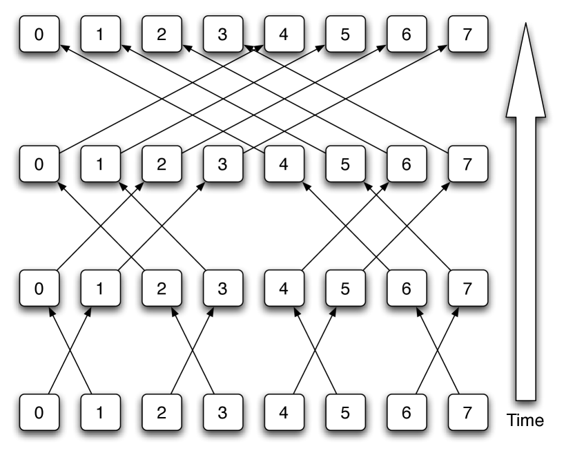
Figure 4: Diagram of a parallel butterfly all-reduction on a binary tree of eight processors. Each arrow represents a message from one processor to another. Time moves upwards.

The reduce-broadcast implementation requires about twice as many stages as the butterfly pattern (in the case of a binary tree) and thus as much as twice the latency. However, it reduces the total number of messages communicated per level of the tree (not just the messages on the critical path). In the case of a binary tree, reduce-broadcast requires at most $P/2$ messages at any one level, and $P\log(P)/2$ total messages. A butterfly always generates $P$ messages at every level, and requires $P\log(P)$ total messages. The choice between reduce-broadcast and butterfly depends on the properties of the communication network.

5.3 TSQR-specific (all-) reduction requirements

TSQR uses an (all-) reduction communication pattern, but has requirements that differ from the standard (all-) reduction. For example, if the $Q$ factor is desired, then TSQR must store intermediate results (the local $Q$ factor from each level’s computation with neighbors) at interior nodes of the tree. This requires reifying and preserving the (all-) reduction tree for later invocation by users. Typical (all-) reduction interfaces, such as those provided by MPI or OpenMP, do not allow this (see e.g., [gropp1999using]). They may not even guarantee that the same tree will be used upon successive invocations of the same (all-) reduction operation, or that the inputs to a node of the (all-) reduction tree will always be in the same order.

6 Optimizations for local QR factorizations

Although TSQR achieves its performance gains because it optimizes communication, the local QR factorizations lie along the critical path of the algorithm. The parallel cluster benchmark results in Section 12 show that optimizing the local QR factorizations can improve performance significantly. In this section, we outline a few of these optimizations, and hint at how they affect the formulation of the general CAQR algorithm in Section 13.

6.1 Structured QR factorizations

Many of the inputs to the local QR factorizations have a particular structure. In the parallel case, they are vertical stacks of $n\times n$ upper triangular matrices, and in the sequential case, at least one of the blocks is upper triangular. In this section, we show how to modify a standard dense Householder QR factorization in order to exploit this structure. This can save a factor of $5\times$ flops and (at least) $3\times$ storage, in the parallel case, and a factor of $2\times$ flops and (up to) $2\times$ storage in the sequential case. We also show how to perform the trailing matrix update with these structured QR factorizations, as it will be useful for Section 13.

Suppose that we have two upper triangular matrices $R_{0}$ and $R_{1}$, each of size $5\times 5$. (The notation here is generic and not meant to correspond to a specific stage of TSQR. This is extended easily enough to the case of $q$ upper triangular matrices, for $q=2,3,\dots$.) Then, we can write their vertical concatenation as follows, in which an $x$ denotes a structural nonzero of the matrix, and empty spaces denote zeros:

$$\begin{pmatrix}R_{0}\\ R_{1}\\ \end{pmatrix}=\begin{pmatrix}x&x&x&x&x\\ &x&x&x&x\\ &&x&x&x\\ &&&x&x\\ &&&&x\\ x&x&x&x&x\\ &x&x&x&x\\ &&x&x&x\\ &&&x&x\\ &&&&x\\ \end{pmatrix}.$$ (3)

Note that we do not need to store the ones on the diagonal explicitly. The $Q$ factor effectively overwrites $R_{1}$ and the $R$ factor overwrites $R_{0}$.

The approach used for performing the QR factorization of the first block column affects the storage for the Householder vectors as well as the update of any trailing matrices that may exist. In general, Householder transformations have the form $I-\tau_{j}v_{j}v_{j}^{T}$, in which the Householder vector $v_{i}$ is normalized so that $v_{i}(1)=1$. This means that $v_{i}(1)$ need not be stored explicitly. Furthermore, if we use structured Householder transformations, we can avoid storing and computing with the zeros in Equation (3). As the Householder vector always has the same nonzero pattern as the vector from which it is calculated, the nonzero structure of the Householder vector is trivial to determine.

For a $2n\times n$ rectangular matrix composed of $n\times n$ upper triangular matrices, the $i$-th Householder vector $v_{i}$ in the QR factorization of the matrix is a vector of length $2n$ with nonzeros in entries $n+1$ through $n+i$, a one in entry $i$, and zeros elsewhere. If we stack all $n$ Householder vectors into a $2n\times n$ matrix, we obtain the following representation of the $Q$ factor (not including the $\tau$ array of multipliers):

$$\begin{pmatrix}1&&&&\\ &1&&&\\ &&1&&\\ &&&1&\\ &&&&1\\ x&x&x&x&x\\ &x&x&x&x\\ &&x&x&x\\ &&&x&x\\ &&&&x\\ \end{pmatrix}.$$ (4)

Algorithm 1 Sequential QR factorization of $qn\times n$ matrix $A$, with structure as in Equation (3)

1:

2:for $j=1$ to $n$ do

3:

4:Let $\mathcal{I}_{j}$ be the index set $\{j$, $n+1:n+j$, $\dots$, $(q-1)n+1:(q-1)n+j\}$

5:

6:$w:=A(\mathcal{I}_{j},j)$$\triangleright$ Gather pivot column of $A$ into $w$

7:

8:$[\tau_{j},v]:=\operatorname{House}(w)$$\triangleright$ Compute Householder reflection, normalized so that $v(1)=1$

9:

10:$X:=A(\mathcal{I}_{j},j+1:n)$$\triangleright$ Gather from $A$ into $X$. One would normally perform the update in place; we use a copy to improve clarity.

11:

12:$X:=(I-\tau_{j}vv^{T})X$$\triangleright$ Apply Householder reflection

13:

14:$A(\mathcal{I}_{j}\setminus\{j\},j):=v(2:end)$$\triangleright$ Scatter $v(2:end)$ back into $A$

15:

16:$A(\mathcal{I}_{j},j+1:n):=X$$\triangleright$ Scatter $X$ back into $A$

17:end for

Algorithm 1 shows a standard, column-by-column sequential QR factorization of the $qn\times n$ matrix of upper triangular $n\times n$ blocks, using structured Householder reflectors. To analyze the cost, consider the components:

1. $\operatorname{House}(w)$: the cost of this is dominated by finding the norm of the vector $w$ and scaling it.

2. Applying a length $n$ Householder reflector, whose vector contains $k$ nonzeros, to an $n\times b$ matrix $A$. This is an operation $(I-\tau vv^{T})A=A-v(\tau(v^{T}A))$.

Appendix LABEL:S:localQR-flops counts the arithmetic operations in detail. There, we find that the total cost is about

$$\frac{2}{3}(q-1)n^{3}$$

flops, to factor a $qn\times n$ matrix (we showed the specific case $q=2$ above). The flop count increases by about a factor of $3\times$ if we ignore the structure of the inputs.

6.2 BLAS 3 structured Householder QR

Algorithm 2 Computing $Y$ and $T$ in the $(Y,T)$ representation of a collection of $n$ Householder reflectors. Modification of an algorithm in [schreiber1989storage] so that $P_{j}=I-\tau_{j}v_{j}v_{j}^{T}$.

1:$n$ Householder reflectors $\rho_{j}=I-\tau_{j}v_{j}v_{j}^{T}$

2:

3:for $j=1$ to $n$ do

4:

5:if $j=1$ then

6:

7:$Y:=[v_{1}]$

8:

9:$T:=[-\tau_{j}]$

10:

11:else

12:

13:$z:=-\tau_{j}(T(Y^{T}v_{j}))$

14:

15:$Y:=\begin{pmatrix}Y&v_{j}\end{pmatrix}$

16:

17:$T:=\begin{pmatrix}T&z\\ 0&-\tau_{j}\\ \end{pmatrix}$

18:end if

19:end for

20:$Y$ and $T$ satisfy $\rho_{1}\cdot\rho_{2}\cdot\dots\rho_{n}=I+YTY^{T}$

Representing the local $Q$ factor as a collection of Householder transforms means that the local QR factorization is dominated by BLAS 2 operations (dense matrix-vector products). A number of authors have shown how to reformulate the standard Householder QR factorization so as to coalesce multiple Householder reflectors into a block, so that the factorization is dominated by BLAS 3 operations. For example, Schreiber and Van Loan describe a so-called YT representation of a collection of Householder reflectors [schreiber1989storage]. BLAS 3 transformations like this are now standard in LAPACK and ScaLAPACK.

We can adapt these techniques in a straightforward way in order to exploit the structured Householder vectors depicted in Equation (4). Schreiber and Van Loan use a slightly different definition of Householder reflectors: $\rho_{j}=I-2v_{j}v_{j}^{T}$, rather than LAPACK’s $\rho_{j}=I-\tau_{j}v_{j}v_{j}^{T}$. Schreiber and Van Loan’s $Y$ matrix is the matrix of Householder vectors $Y=[v_{1}\,v_{2}\,\dots\,v_{n}]$; its construction requires no additional computation as compared with the usual approach. However, the $T$ matrix must be computed, which increases the flop count by a constant factor. The cost of computing the $T$ factor for the $qn\times n$ factorization above is about $qn^{3}/3$. Algorithm 2 shows the resulting computation. Note that the $T$ factor requires $n(n-1)/2$ additional storage per processor on which the $T$ factor is required.

6.3 Recursive Householder QR

In Section 12, we show large performance gains obtained by using Elmroth and Gustavson’s recursive algorithm for the local QR factorizations [elmroth2000applying]. The authors themselves observed that their approach works especially well with “tall thin” matrices, and others have exploited this effect in their applications (see e.g., [rabani2001outcore]). The recursive approach outperforms LAPACK because it makes the panel factorization a BLAS 3 operation. In LAPACK, the panel QR factorization consists only of matrix-vector and vector-vector operations. This suggests why recursion helps especially well with tall, thin matrices. Elmroth and Gustavson’s basic recursive QR does not perform well when $n$ is large, as the flop count grows cubically in $n$, so they opt for a hybrid approach that divides the matrix into panels of columns, and performs the panel QR factorizations using the recursive method.

Elmroth and Gustavson use exactly the same representation of the $Q$ factor as Schreiber and Van Loan [schreiber1989storage], so the arguments of the previous section still apply.

6.4 Trailing matrix update

Section 13 will describe how to use TSQR to factor matrices in general 2-D layouts. For these layouts, once the current panel (block column) has been factored, the panels to the right of the current panel cannot be factored until the transpose of the current panel’s $Q$ factor has been applied to them. This is called a trailing matrix update. The update lies along the critical path of the algorithm, and consumes most of the floating-point operations in general. This holds regardless of whether the factorization is left-looking, right-looking, or some hybrid of the two. Thus, it’s important to make the updates efficient.

The trailing matrix update consists of a sequence of applications of local $Q^{T}$ factors to groups of “neighboring” trailing matrix blocks. (Section 5 explains the meaning of the word “neighbor” here.) We now explain how to do one of these local $Q^{T}$ applications. (Do not confuse the local $Q$ factor, which we label generically as $Q$, with the entire input matrix’s $Q$ factor.)

Let the number of rows in a block be $M$, and the number of columns in a block be $N$. We assume $M\geq N$. Suppose that we want to apply the local $Q^{T}$ factor from the above $qN\times N$ matrix factorization, to two blocks $C_{0}$ and $C_{1}$ of a trailing matrix panel. (This is the case $q=2$, which we assume for simplicity.) We divide each of the $C_{i}$ into a top part and a bottom part:

$$C_{i}=\begin{pmatrix}C_{i}(1:N,:)\\ C_{i}(N+1:M,:)\end{pmatrix}=\begin{pmatrix}C_{i}^{\prime}\\ C_{i}^{\prime\prime}\end{pmatrix}.$$

Our goal is to perform the operation

$$\begin{pmatrix}R_{0}&C_{0}^{\prime}\\ R_{1}&C_{1}^{\prime}\\ \end{pmatrix}=\begin{pmatrix}QR&C_{0}^{\prime}\\ &C_{1}^{\prime}\\ \end{pmatrix}=Q\cdot\begin{pmatrix}R&\hat{C}_{0}^{\prime}\\ &\hat{C}_{1}^{\prime}\\ \end{pmatrix},$$

in which $Q$ is the local $Q$ factor and $R$ is the local $R$ factor of $[R_{0};R_{1}]$. Implicitly, the local $Q$ factor has the dimensions $2M\times 2M$, as Section 4 explains. However, it is not stored explicitly, and the implicit operator that is stored has the dimensions $2N\times 2N$. We assume that processors $P_{0}$ and $P_{1}$ each store a redundant copy of $Q$, that processor $P_{2}$ has $C_{0}$, and that processor $P_{3}$ has $C_{1}$. We want to apply $Q^{T}$ to the matrix

$$C=\begin{pmatrix}C_{0}\\ C_{1}\\ \end{pmatrix}.$$

First, note that $Q$ has a specific structure. If stored explicitly, it would have the form

$$Q=\begin{pmatrix}\begin{matrix}U_{00}&\\ &I_{M-N}\end{matrix}&\begin{matrix}U_{01}&\\ &\mathbf{0}_{M-N}\end{matrix}\\ \begin{matrix}U_{10}&\\ &\mathbf{0}_{M-N}\end{matrix}&\begin{matrix}U_{11}&\\ &I_{M-N}\end{matrix}\\ \end{pmatrix},$$

in which the $U_{ij}$ blocks are each $N\times N$. This makes the only nontrivial computation when applying $Q^{T}$ the following:

$$\begin{pmatrix}\hat{C}_{0}^{\prime}\\ \hat{C}_{1}^{\prime}\\ \end{pmatrix}:=\begin{pmatrix}U_{00}^{T}&U_{10}^{T}\\ U_{01}^{T}&U_{11}^{T}\end{pmatrix}\cdot\begin{pmatrix}C_{0}^{\prime}\\ C_{1}^{\prime}\\ \end{pmatrix}.$$ (5)

We see, in particular, that only the uppermost $N$ rows of each block of the trailing matrix need to be read or written. Note that it is not necessary to construct the $U_{ij}$ factors explicitly; we need only operate on $C_{0}^{\prime}$ and $C_{1}^{\prime}$ with $Q^{T}$.

If we are using a standard Householder QR factorization (without BLAS 3 optimizations), then computing Equation (5) is straightforward. When one wishes to exploit structure (as in Section 6.1) and use a local QR factorization that exploits BLAS 3 operations (as in Section 6.2), more interesting load balance issues arise. We will discuss these in the following section.

6.4.1 Trailing matrix update with structured BLAS 3 QR

An interesting attribute of the YT representation is that the $T$ factor can be constructed using only the $Y$ factor and the $\tau$ multipliers. This means that it is unnecessary to send the $T$ factor for updating the trailing matrix; the receiving processors can each compute it themselves. However, one cannot compute $Y$ from $T$ and $\tau$ in general.

When the YT representation is used, the update of the trailing matrices takes the following form:

$$\begin{pmatrix}\hat{C_{0}}^{\prime}\\ \hat{C_{1}}^{\prime}\\ \end{pmatrix}:=\begin{pmatrix}I-\begin{pmatrix}I\\ Y_{1}\\ \end{pmatrix}\cdot\begin{array}[]{cc}T^{T}\\ \\ \end{array}\cdot\begin{pmatrix}I\\ Y_{1}\\ \end{pmatrix}^{T}\end{pmatrix}\begin{pmatrix}C_{0}^{\prime}\\ C_{1}^{\prime}\\ \end{pmatrix}.$$

Here, $Y_{1}$ starts on processor $P_{1}$, $C_{0}^{\prime}$ on processor $P_{2}$, and $C_{1}^{\prime}$ on processor $P_{3}$. The matrix $T$ must be computed from $\tau$ and $Y_{1}$; we can assume that $\tau$ is on processor $P_{1}$. The updated matrices $\hat{C_{0}}^{\prime}$ and $\hat{C_{1}}^{\prime}$ are on processors $P_{2}$ resp. $P_{3}$.

There are many different ways to perform this parallel update. The data dependencies impose a directed acyclic graph (DAG) on the flow of data between processors. One can find the the best way to do the update by realizing an optimal computation schedule on the DAG. Our performance models can be used to estimate the cost of a particular schedule.

Here is a straightforward but possibly suboptimal schedule. First, assume that $Y_{1}$ and $\tau$ have already been sent to $P_{3}$. Then,

$P_{2}$’s tasks:

• Send $C_{0}^{\prime}$ to $P_{3}$

• Receive $W$ from $P_{3}$

• Compute $\hat{C_{0}}^{\prime}=C_{0}^{\prime}-W$

$P_{3}$’s tasks:

• Compute the $T$ factor and $W:=T^{T}(C_{0}^{\prime}+Y_{1}^{T}C_{1}^{\prime})$

• Send $W$ to $P_{2}$

• Compute $\hat{C_{1}}^{\prime}:=C_{1}^{\prime}-Y_{1}W$

However, this leads to some load imbalance, since $P_{3}$ performs more computation than $P_{2}$. It does not help to compute $T$ on $P_{0}$ or $P_{1}$ before sending it to $P_{3}$, because the computation of $T$ lies on the critical path in any case. We will see in Section 13 that part of this computation can be overlapped with the communication.

For $q\geq 2$, we can write the update operation as

$$\begin{pmatrix}\hat{C_{0}}^{\prime}\\ \hat{C_{1}}^{\prime}\\ \vdots\\ \hat{C_{q-1}}^{\prime}\\ \end{pmatrix}:=\left(I-\begin{pmatrix}I_{N\times N}\\ Y_{1}\\ \vdots\\ Y_{q-1}\\ \end{pmatrix}T^{T}\begin{pmatrix}I_{N\times N}&Y_{1}^{T}&\dots&Y_{q-1}^{T}\\ \end{pmatrix}\right)\begin{pmatrix}C_{0}^{\prime}\\ C_{1}^{\prime}\\ \vdots\\ C_{q-1}^{\prime}\\ \end{pmatrix}.$$

If we let

$$D:=C_{0}^{\prime}+Y_{1}^{T}C_{1}^{\prime}+Y_{2}^{T}C_{2}^{\prime}+\dots+Y_{q-1}^{T}C_{q-1}^{\prime}$$

be the “inner product” part of the update operation formulas, then we can rewrite the update formulas as

$$\hat{C_{0}}^{\prime} :=C_{0}^{\prime}-T^{T}D,$$

$$\hat{C_{1}}^{\prime} :=C_{1}^{\prime}-Y_{1}T^{T}D,$$

$$\vdots$$

$$\hat{C_{q-1}}^{\prime} :=C_{q-1}^{\prime}-Y_{q-1}T^{T}D.$$

As the branching factor $q$ gets larger, the load imbalance becomes less of an issue. The inner product $D$ should be computed as an all-reduce in which the processor owning $C_{i}$ receives $Y_{i}$ and $T$. Thus, all the processors but one will have the same computational load.

7 Machine model

7.1 Parallel machine model

Throughout this work, we use the “alpha-beta” or latency-bandwidth model of communication, in which a message of size $n$ floating-point words takes time $\alpha+\beta n$ seconds. The $\alpha$ term represents message latency (seconds per message), and the $\beta$ term inverse bandwidth (seconds per floating-point word communicated). Our algorithms only need to communicate floating-point words, all of the same size. We make no attempt to model overlap of communication and computation, but we do mention the possibility of overlap when it exists. Exploiting overlap could potentially speed up our algorithms (or any algorithm) by a factor of two.

We predict floating-point performance by counting floating-point operations and multiplying them by $\gamma$, the inverse peak floating-point performance, also known as the floating-point throughput. The quantity $\gamma$ has units of seconds per flop (so it can be said to measure the bandwidth of the floating-point hardware). If we need to distinguish between adds and multiplies on one hand, and divides on the other, we use $\gamma$ for the throughput of adds and multiplies, and $\gamma_{d}$ for the throughput of divides.

When appropriate, we may scale the peak floating-point performance prediction of a particular matrix operation by a factor, in order to account for the measured best floating-point performance of local QR factorizations. This generally gives the advantage to competing algorithms rather than our own, as our algorithms are designed to perform better when communication is much slower than arithmetic.

7.2 Sequential machine model

We also apply the alpha-beta model to communication between levels of the memory hierarchy in the sequential case. We restrict our model to describe only two levels at one time: fast memory (which is smaller) and slow memory (which is larger). The terms “fast” and “slow” are always relative. For example, DRAM may be considered fast if the slow memory is disk, but DRAM may be considered slow if the fast memory is cache. As in the parallel case, the time to complete a transfer between two levels is modeled as $\alpha+\beta n$. We assume that user has explicit control over data movement (reads and writes) between fast and slow memory. This offers an upper bound when control is implicit (as with caches), and also allows our model as well as our algorithms to extend to systems like the Cell processor (in which case fast memory is an individual local store, and slow memory is DRAM).

We assume that the fast memory can hold $W$ floating-point words. For any QR factorization operating on an $m\times n$ matrix, the quantity

$$\frac{mn}{W}$$

bounds from below the number of loads from slow memory into fast memory (as the method must read each entry of the matrix at least once). It is also a lower bound on the number of stores from fast memory to slow memory (as we assume that the algorithm must write the computed $Q$ and $R$ factors back to slow memory). Sometimes we may refer to the block size $P$. In the case of TSQR, we usually choose

$$P=\frac{mn}{3W},$$

since at most three blocks of size $P$ must be in fast memory at one time when applying the $Q$ or $Q^{T}$ factor in sequential TSQR (see Section 4).

In the sequential case, just as in the parallel case, we assume all memory transfers are nonoverlapped. Overlapping communication and computation may provide up to a twofold performance improvement. However, some implementations may consume fast memory space in order to do buffering correctly. This matters because the main goal of our sequential algorithms is to control fast memory usage, often to solve problems that do not fit in fast memory. We usually want to use as much of fast memory as possible, in order to avoid expensive transfers to and from slow memory.

8 TSQR implementation

In this section, we describe the TSQR factorization algorithm in detail. We also build a performance model of the algorithm, based on the machine model in Section 7 and the operation counts of the local QR factorizations in Section 6. Parallel TSQR performs $2mn^{2}/P+\frac{2n^{3}}{3}\log P$ flops, compared to the $2mn^{2}/P-2n^{3}/(3P)$ flops performed by ScaLAPACK’s parallel QR factorization PDGEQRF, but requires $2n$ times fewer messages. The sequential TSQR factorization performs the same number of flops as sequential blocked Householder QR, but requires $\Theta(n)$ times fewer transfers between slow and fast memory, and a factor of $\Theta(m/\sqrt{W})$ times fewer words transferred, in which $W$ is the fast memory size.

8.1 Reductions and all-reductions

In Section 5, we gave a detailed description of (all-)reductions. We did so because the TSQR factorization is itself an (all-)reduction, in which additional data (the components of the $Q$ factor) is stored at each node of the (all-)reduction tree. Applying the $Q$ or $Q^{T}$ factor is also a(n) (all-)reduction.

If we implement TSQR with an all-reduction, then we get the final $R$ factor replicated over all the processors. This is especially useful for Krylov subspace methods. If we implement TSQR with a reduction, then the final $R$ factor is stored only on one processor. This avoids redundant computation, and is useful both for block column factorizations for 2-D block (cyclic) matrix layouts, and for solving least squares problems when the $Q$ factor is not needed.

8.2 Factorization

We now describe the parallel and sequential TSQR factorizations for the 1-D block row layout. (We omit the obvious generalization to a 1-D block cyclic row layout.)

Parallel TSQR computes an $R$ factor which is duplicated over all the processors, and a $Q$ factor which is stored implicitly in a distributed way. The algorithm overwrites the lower trapezoid of $A_{i}$ with the set of Householder reflectors for that block, and the $\tau$ array of scaling factors for these reflectors is stored separately. The matrix $R_{i,k}$ is stored as an $n\times n$ upper triangular matrix for all stages $k$. Algorithm 3 shows an implementation of parallel TSQR, based on an all-reduction. (Note that running Algorithm 3 on a matrix stored in a 1-D block cyclic layout still works, though it performs an implicit block row permutation on the $Q$ factor.)

Algorithm 3 Parallel TSQR

1:$\Pi$ is the set of $P$ processors

2:All-reduction tree with height $L$. If $P$ is a power of two and we want a binary all-reduction tree, then $L=\log_{2}P$.

3:$i\in\Pi$: my processor’s index

4:The $m\times n$ input matrix $A$ is distributed in a 1-D block row layout over the processors; $A_{i}$ is the block of rows belonging to processor $i$.

5:

6:Compute $[Q_{i,0},R_{i,0}]:=qr(A_{i})$ using sequential Householder QR

7:

8:for $k$ from 1 to $L$ do

9:

10:if I have any neighbors in the all-reduction tree at this level then

11:

12:Send (non-blocking) $R_{i,k-1}$ to each neighbor not myself

13:

14:Receive (non-blocking) $R_{j,k-1}$ from each neighbor $j$ not myself

15:

16:Wait until the above sends and receives complete$\triangleright$ Note: not a global barrier.

17:

18:Stack the upper triangular $R_{j,k-1}$ from all neighbors (including my own $R_{i,k-1}$), by order of processor ids, into a $qn\times n$ array $C$, in which $q$ is the number of neighbors.

19:

20:Compute $[Q_{i,k},R_{i,k}]:=qr(C)$ using Algorithm 1 in Section 6.1

21:

22:else

23:

24:$R_{i,k}:=R_{i,k-1}$

25:

26:$Q_{i,k}:=I_{n\times n}$$\triangleright$ Stored implicitly

27:end if

28:

29:Processor $i$ has an implicit representation of its block column of $Q_{i,k}$. The blocks in the block column are $n\times n$ each and there are as many of them as there are neighbors at stage $k$ (including $i$ itself). We don’t need to compute the blocks explicitly here.

30:end for

31:$R_{i,L}$ is the $R$ factor of $A$, for all processors $i\in\Pi$.

32:The $Q$ factor is implicitly represented by $\{Q_{i,k}\}$: $i\in\Pi$, $k\in\{0,1,\dots,L\}\}$.

Sequential TSQR begins with an $m\times n$ matrix $A$ stored in slow memory. The matrix $A$ is divided into $P$ blocks $A_{0}$, $A_{1}$, $\dots$, $A_{P-1}$, each of size $m/P\times n$. (Here, $P$ has nothing to do with the number of processors.) Each block of $A$ is loaded into fast memory in turn, combined with the $R$ factor from the previous step using a QR factorization, and the resulting $Q$ factor written back to slow memory. Thus, only one $m/P\times n$ block of $A$ resides in fast memory at one time, along with an $n\times n$ upper triangular $R$ factor. Sequential TSQR computes an $n\times n$ $R$ factor which ends up in fast memory, and a $Q$ factor which is stored implicitly in slow memory as a set of blocks of Householder reflectors. Algorithm 4 shows an implementation of sequential TSQR.

Algorithm 4 Sequential TSQR

1:The $m\times n$ input matrix $A$, stored in slow memory, is divided into $P$ row blocks $A_{0}$, $A_{1}$, $\dots$, $A_{P-1}$

2:

3:Load $A_{0}$ into fast memory

4:

5:Compute $[Q_{00},R_{00}]:=qr(A_{0})$ using standard sequential QR. Here, the $Q$ factor is represented implicitly by an $m/P\times n$ lower triangular array of Householder reflectors $Y_{00}$ and their $n$ associated scaling factors $\tau_{00}$

6:

7:Write $Y_{00}$ and $\tau_{00}$ back to slow memory; keep $R_{00}$ in fast memory

8:

9:for $k=1$ to $P-1$ do

10:

11:Load $A_{k}$

12:

13:Compute $[Q_{01},R_{01}]=qr([R_{0,k-1};A_{k}])$ using the structured method analyzed in Appendix LABEL:SSS:localQR-flops:seq:2blocks. Here, the $Q$ factor is represented implicitly by a full $m/P\times n$ array of Householder reflectors $Y_{0k}$ and their $n$ associated scaling factors $\tau_{0k}$.

14:

15:Write $Y_{0k}$ and $\tau_{0k}$ back to slow memory; keep $R_{0k}$ in fast memory

16:end for

17:$R_{0,P-1}$ is the $R$ factor in the QR factorization of $A$, and is in fast memory

18:The $Q$ factor is implicitly represented by $Q_{00}$, $Q_{01}$, $\dots$, $Q_{0,P-1}$, and is in slow memory

8.2.1 Performance model

In Appendix LABEL:S:TSQR-par-detailed, we develop a performance model for parallel TSQR on a binary tree. Appendix LABEL:S:TSQR-seq-detailed does the same for sequential TSQR on a flat tree.

A parallel TSQR factorization on a binary reduction tree performs the following computations along the critical path: One local QR factorization of a fully dense $m/P\times n$ matrix, and $\log P$ factorizations, each of a $2n\times n$ matrix consisting of two $n\times n$ upper triangular matrices. The factorization requires

$$\frac{2mn^{2}}{P}+\frac{2n^{3}}{3}\log P$$

flops and $\log P$ messages, and transfers a total of $(1/2)n^{2}\log P$ words between processors. In contrast, parallel Householder QR requires

$$\frac{2mn^{2}}{P}-\frac{2n^{3}}{3}$$

flops and $2n\log P$ messages, but also transfers $(1/2)n^{2}\log P$ words between processors. For details, see Table 10 in Section 9.

Sequential TSQR on a flat tree performs the same number of flops as sequential Householder QR, namely

$$2mn^{2}-\frac{2n^{3}}{3}$$

flops. However, sequential TSQR only transfers

$$2mn-\frac{n(n+1)}{2}+\frac{mn^{2}}{\tilde{W}}$$

words between slow and fast memory, in which $\tilde{W}=W-n(n+1)/2$, and only performs

$$\frac{2mn}{\tilde{W}}$$

transfers between slow and fast memory. In contrast, blocked sequential Householder QR transfers

$$\frac{m^{2}n^{2}}{2W}-\frac{mn^{3}}{6W}+\frac{3mn}{2}-\frac{3n^{2}}{4}$$

words between slow and fast memory, and only performs

$$\frac{2mn}{W}+\frac{mn^{2}}{2W}$$

transfers between slow and fast memory. For details, see Table 11 in Section 9.

8.3 Applying $Q$ or $Q^{T}$ to vector(s)

Just like Householder QR, TSQR computes an implicit representation of the $Q$ factor. One need not generate an explicit representation of $Q$ in order to apply the $Q$ or $Q^{T}$ operators to one or more vectors. In fact, generating an explicit $Q$ matrix requires just as many messages as applying $Q$ or $Q^{T}$. (The performance model for applying $Q$ or $Q^{T}$ is an obvious extension of the factorization performance model; the parallel performance model is developed in Appendix LABEL:SS:TSQR-par-detailed:apply and the sequential performance model in Appendix LABEL:SS:TSQR-seq-detailed:apply.) Furthermore, the implicit representation can be updated or downdated, by using standard techniques (see e.g., [govl:96]) on the local QR factorizations recursively. The $s$-step Krylov methods mentioned in Section 3 employ updating and downdating extensively.

In the case of the “thin” $Q$ factor (in which the vector input is of length $n$), applying $Q$ involves a kind of broadcast operation (which is the opposite of a reduction). If the “full” $Q$ factor is desired, then applying $Q$ or $Q^{T}$ is a kind of all-to-all (like the fast Fourier transform). Computing $Q\cdot x$ runs through the nodes of the (all-)reduction tree from leaves to root, whereas computing $Q^{T}\cdot y$ runs from root to leaves.

9 Other “tall skinny” QR algorithms

There are many other algorithms besides TSQR for computing the QR factorization of a tall skinny matrix. They differ in terms of performance and accuracy, and may store the $Q$ factor in different ways that favor certain applications over others. In this section, we model the performance of the following competitors to TSQR:

• Four different Gram-Schmidt variants

• CholeskyQR (see [stwu:02])

• Householder QR, with a block row layout

Each includes parallel and sequential versions. For Householder QR, we base our parallel model on the ScaLAPACK routine PDGEQRF, and the sequential model on left-looking blocked Householder. Our left-looking blocked Householder implementation is modeled on the out-of-core ScaLAPACK routine PFDGEQRF, which is left-looking instead of right-looking in order to minimize the number of writes to slow memory (the total amount of data moved between slow and fast memory is the same for both left-looking and right-looking blocked Householder QR). See Appendix LABEL:S:PFDGEQRF for details. In the subsequent Section 10, we summarize the numerical accuracy of these QR factorization methods, and discuss their suitability for different applications.

In the parallel case, CholeskyQR and TSQR have comparable numbers of messages and communicate comparable numbers of words, but CholeskyQR requires a constant factor fewer flops along the critical path. However, the $Q$ factor computed by TSQR is always numerically orthogonal, whereas the $Q$ factor computed by CholeskyQR loses orthogonality proportionally to $\kappa_{2}(A)^{2}$. The variants of Gram-Schmidt require at best a factor $n$ more messages than these two algorithms, and lose orthogonality at best proportionally to $\kappa_{2}(A)$.

9.1 Gram-Schmidt orthogonalization

Gram-Schmidt has two commonly used variations: “classical” (CGS) and “modified” (MGS). Both versions have the same floating-point operation count, but MGS performs them in a different order to improve stability. We will show that a parallel implementation of MGS uses at best $2n\log P$ messages, in which $P$ is the number of processors, and a blocked sequential implementation requires at least

$$\frac{mn^{2}}{2W-n(n+1)}$$

transfers between slow and fast memory, in which $W$ is the fast memory capacity. In contrast, parallel TSQR requires only $\log P$ messages, and sequential TSQR only requires

$$\frac{4mn}{2W-n(n+1)}$$

transfers between slow and fast memory, a factor of about $n/4$ less. See Tables 7 and 8 for details.

9.1.1 Left- and right-looking

Just like many matrix factorizations, both MGS and CGS come in left-looking and right-looking variants. To distinguish between the variants, we append “_L” resp. “_R” to the algorithm name to denote left- resp. right-looking. We show all four combinations as Algorithms 5–8. Both right-looking and left-looking variants loop from left to right over the columns of the matrix $A$. At iteration $k$ of this loop, the left-looking version only accesses columns $1$ to $k$ inclusive, whereas the right-looking version only accesses columns $k$ to $n$ inclusive. Thus, right-looking algorithms require the entire matrix to be available, which forbids their use when the matrix is to be generated and orthogonalized one column at a time. (In this case, only left-looking algorithms may be used.) We assume here that the entire matrix is available at the start of the algorithm.

Right-looking Gram-Schmidt is usually called “row-oriented Gram-Schmidt,” and by analogy, left-looking Gram-Schmidt is usually called “column-oriented Gram-Schmidt.” We use the terms “right-looking” resp. “left-looking” for consistency with the other QR factorization algorithms in this paper.

Algorithm 5 Modified Gram-Schmidt, right-looking

1:$A$: $m\times n$ matrix with $m\geq n$

2:

3:for $k=1$ to $n$ do

4:

5:$R(k,k):=\|A(:,k)\|_{2}$

6:

7:$Q(:,k):=A(:,k)/R(k,k)$

8:

9:$R(k,k+1:n):=Q(:,k)^{T}\cdot A(:,k+1:n)$

10:

11:$A(:,k+1:n):=A(:,k+1:n)-R(k,k+1:n)\cdot Q(:,k)$

12:end for

Algorithm 6 Modified Gram-Schmidt, left-looking

1:$A$: $m\times n$ matrix with $m\geq n$

2:

3:for $k=1$ to $n$ do

4:

5:$v:=A(:,k)$

6:

7:for $j=1$ to $k-1$ do$\triangleright$ Data dependencies hinder vectorization

8:

9:$R(j,k):=Q(:,j)^{T}\cdot v$$\triangleright$ Change $v$ to $A(:,k)$ to get CGS

10:

11:$v:=v-R(j,k)\cdot Q(:,j)$

12:end for

13:

14:$R(k,k):=\|v\|_{2}$

15:

16:$Q(:,k):=v/R(k,k)$

17:end for

Algorithm 7 Classical Gram-Schmidt, right-looking

1:$A$: $m\times n$ matrix with $m\geq n$

2:

3:$V:=A$$\triangleright$ Not copying $A$ would give us right-looking MGS.

4:

5:for $k=1$ to $n$ do

6:

7:$R(k,k):=\|V(:,k)\|_{2}$

8:

9:$Q(:,k):=V(:,k)/R(k,k)$

10:

11:$R(k,k+1:n):=Q(:,k)^{T}\cdot A(:,k+1:n)$

12:

13:$V(:,k+1:n):=V(:,k+1:n)-R(k,k+1:n)\cdot Q(:,k)$

14:end for

Algorithm 8 Classical Gram-Schmidt, left-looking

1:$A$: $m\times n$ matrix with $m\geq n$

2:

3:for $k=1$ to $n$ do

4:

5:$R(1:k-1,k):=Q(:,1:k-1)^{T}\cdot A(:,k)$$\triangleright$ This and the next statement are not vectorized in left-looking MGS.

6:

7:$A(:,k):=A(:,k)-R(1:k-1,k)\cdot Q(:,1:k-1)$$\triangleright$ In the sequential case, one can coalesce the read of each block of $A(:,k)$ in this statement with the read of each block of $A(:,k)$ in the next statement.

8:

9:$R(k,k):=\|A(:,k)\|_{2}$

10:

11:$Q(:,k):=A(:,k)/R(k,k)$

12:end for

9.1.2 Reorthogonalization

One can improve the stability of CGS by reorthogonalizing the vectors. The simplest way is to make two orthogonalization passes per column, that is, to orthogonalize the current column against all the previous columns twice. We call this “CGS2.” This method only makes sense for left-looking Gram-Schmidt, when there is a clear definition of “previous columns.” Normally one would orthogonalize the column against all previous columns once, and then use some orthogonality criterion to decide whether to reorthogonalize the column. As a result, the performance of CGS2 is data-dependent, so we do not model its performance here. In the worst case, it can cost twice as much as CGS_L. Section 10 discusses the numerical stability of CGS2 and why “twice is enough.”

9.1.3 Parallel Gram-Schmidt

MGS_L (Algorithm 6) requires about $n/4$ times more messages than MGS_R (Algorithm 5), since the left-looking algorithm’s data dependencies prevent the use of matrix-vector products. CGS_R (Algorithm 7) requires copying the entire input matrix; not doing so results in MGS_R (Algorithm 5), which is more numerically stable in any case. Thus, for the parallel case, we favor MGS_R and CGS_L for a fair comparison with TSQR.

In the parallel case, all four variants of MGS and CGS listed here require

$$\frac{2mn^{2}}{P}+O\left(\frac{mn}{P}\right)$$

arithmetic operations, and involve communicating

$$\frac{n^{2}}{2}\log(P)+O(n\log(P))$$

floating-point words in total. MGS_L requires

$$\frac{n^{2}}{2}\log(P)+O(n\log(P))$$

messages, whereas the other versions only need $2n\log(P)$ messages. Table 7 shows all four performance models.

Parallel algorithm	# flops	# messages	# words
Right-looking MGS	$2mn^{2}/P$	$2n\log(P)$	$\frac{n^{2}}{2}\log(P)$
Left-looking MGS	$2mn^{2}/P$	$\frac{n^{2}}{2}\log(P)$	$\frac{n^{2}}{2}\log(P)$
Right-looking CGS	$2mn^{2}/P$	$2n\log(P)$	$\frac{n^{2}}{2}\log(P)$
Left-looking CGS	$2mn^{2}/P$	$2n\log(P)$	$\frac{n^{2}}{2}\log(P)$

Table 7: Arithmetic operation counts, number of messages, and total communication volume (in number of words transferred) for parallel left-looking and right-looking variants of CGS and MGS. Reductions are performed using a binary tree on $P$ processors. Lower-order terms omitted.

9.1.4 Sequential Gram-Schmidt

For one-sided factorizations in the out-of-slow-memory regime, left-looking algorithms require fewer writes than their right-looking analogues (see e.g., [toledo99survey]). We will see this in the results below, which is why we spend more effort analyzing the left-looking variants.

Both MGS and CGS can be reorganized into blocked variants that work on panels. These variants perform the same floating-point operations as their unblocked counterparts, but save some communication. In the parallel case, the blocked algorithms encounter the same latency bottleneck as ScaLAPACK’s parallel QR factorization PDGEQRF, so we do not analyze them here. The sequential case offers more potential for communication savings.

The analysis of blocked sequential Gram-Schmidt’s communication costs resembles that of blocked left-looking Householder QR (see Appendix LABEL:S:PFDGEQRF), except that Gram-Schmidt computes and stores the $Q$ factor explicitly. This means that Gram-Schmidt stores the upper triangle of the matrix twice: once for the $R$ factor, and once for the orthogonalized vectors. Left-looking MGS and CGS would use a left panel of width $b$ and a current panel of width $c$, just like blocked left-looking Householder QR. Right-looking Gram-Schmidt would use a current panel of width $c$ and a right panel of width $b$. Unlike Householder QR, however, Gram-Schmidt requires storing the $R$ factor separately, rather than overwriting the original matrix’s upper triangle. We assume here that $W\gg n(n+1)/2$, so that the entire $R$ factor can be stored in fast memory. This need not be the case, but it is a reasonable assumption for the “tall skinny” regime. If $m\approx n$, then Gram-Schmidt’s additional bandwidth requirements, due to working with the upper triangle twice (once for the $Q$ factor and once for the $R$ factor), make Householder QR more competitive than Gram-Schmidt.

For sequential MGS_L, the number of words transferred between slow and fast memory is about

$$\sum_{j=1}{\frac{n}{c}}\left(2cm+\sum{k=1}{\frac{c(j-1)}{b}}bm\right)=\frac{3mn}{2}+\frac{mn^{2}}{2c},$$ (6)

and the number of messages is about

$$\frac{n^{2}}{2bc}+\frac{2n}{c}-\frac{n}{2b}.$$ (7)

The fast memory usage is about $(b+c)m+n(n+1)/2$, so if we optimize for bandwidth and take $b=1$ and

$$c\approx\frac{W-n(n+1)/2}{m},$$

the number of words transferred between slow and fast memory is about

$$\frac{3mn}{2}+\frac{m^{2}n^{2}}{2W-n(n+1)},$$ (8)

and the number of messages is about (using the highest-order term only)

$$\frac{mn^{2}}{2W-n(n+1)}.$$ (9)

For sequential MGS_R, the number of words transferred between slow and fast memory is about

$$\sum_{j=1}^{\frac{n}{c}}\left(2cm+\sum_{k=\frac{c(j-1)}{b}}^{\frac{n}{b}}2bm\right)=3mn+\frac{mn^{2}}{c}+\frac{2bmn}{c}.$$ (10)

This is always greater than the number of words transferred by MGS_L. The number of messages is about

$$\frac{n^{2}}{bc}+\frac{4n}{c}+\frac{n}{b},$$ (11)

which is also always greater than the number of messages transferred by MGS_L. Further analysis is therefore unnecessary; we should always use the left-looking version.

Table 8 shows performance models for blocked versions of left-looking and right-looking sequential MGS and CGS. We omit CGS_R as it requires extra storage and provides no benefits over MGS_R.

Sequential algorithm	# flops	# messages	# words
Right-looking MGS	$2mn^{2}$	$\frac{2mn^{2}}{2W-n(n+1)}$	$3mn+\frac{2mn^{2}}{2W-n(n+1)}$
Left-looking MGS	$2mn^{2}$	$\frac{mn^{2}}{2W-n(n+1)}$	$\frac{3mn}{2}+\frac{m^{2}n^{2}}{2W-n(n+1)}$
Left-looking CGS	$2mn^{2}$	$\frac{mn^{2}}{2W-n(n+1)}$	$\frac{3mn}{2}+\frac{m^{2}n^{2}}{2W-n(n+1)}$

Table 8: Arithmetic operation counts, number of reads and writes, and total communication volume (in number of words read and written) for sequential left-looking CGS and MGS. $W$ is the fast memory capacity in number of floating-point words. Lower-order terms omitted.

9.2 CholeskyQR

Algorithm 9 CholeskyQR factorization

1:$A$: $m\times n$ matrix with $m\geq n$

2:

3:$W:=A^{T}A$$\triangleright$ (All-)reduction

4:

5:Compute the Cholesky factorization $L\cdot L^{T}$ of $W$

6:

7:$Q:=AL^{-T}$

8:$[Q,L^{T}]$ is the QR factorization of $A$

CholeskyQR (Algorithm 9) is a QR factorization that requires only one all-reduction [stwu:02]. In the parallel case, it requires $\log_{2}P$ messages, where $P$ is the number of processors. In the sequential case, it reads the input matrix only once. Thus, it is optimal in the same sense that TSQR is optimal. Furthermore, the reduction operator is matrix-matrix addition rather than a QR factorization of a matrix with comparable dimensions, so CholeskyQR should always be faster than TSQR. Section 12 supports this claim with performance data on a cluster. Note that in the sequential case, $P$ is the number of blocks, and we assume conservatively that fast memory must hold $2mn/P$ words at once (so that $W=2mn/P$).

Algorithm	# flops	# messages	# words
Parallel CholeskyQR	$\frac{2mn^{2}}{P}+\frac{n^{3}}{3}$	$\log(P)$	$\frac{n^{2}}{2}\log(P)$
Sequential CholeskyQR	$2mn^{2}+\frac{n^{3}}{3}$	$\frac{6mn}{W}$	$3mn$

Table 9: Performance model of the parallel and sequential CholeskyQR factorization. We assume $W=2mn/P$ in the sequential case, where $P$ is the number of blocks and $W$ is the number of floating-point words that fit in fast memory. Lower-order terms omitted. All parallel terms are counted along the critical path.

CholeskyQR begins by computing half of the symmetric matrix $A^{T}A$. In the parallel case, each processor $i$ computes half of its component $A_{i}^{T}A_{i}$ locally. In the sequential case, this happens one block at a time. Since this result is a symmetric $n\times n$ matrix, the operation takes only $mn^{2}/P+O(mn/P)$ flops. These local components are then summed using a(n) (all-)reduction, which can also exploit symmetry. The final operation, the Cholesky factorization, requires $n^{3}/3+O(n^{2})$ flops. (Choosing a more stable or robust factorization does not improve the accuracy bound, as the accuracy has already been lost by computing $A^{T}A$.) Finally, the $Q:=AL^{-T}$ operation costs $mn^{2}/P+O(mn/P)$ flops per block of $A$. Table 9 summarizes both the parallel and sequential performance models. In Section 10, we compare the accuracy of CholeskyQR to that of TSQR and other “tall skinny” QR factorization algorithms.

9.3 Householder QR

Householder QR uses orthogonal reflectors to reduce a matrix to upper tridiagonal form, one column at a time (see e.g., [govl:96]). In the current version of LAPACK and ScaLAPACK, the reflectors are coalesced into block columns (see e.g., [schreiber1989storage]). This makes trailing matrix updates more efficient, but the panel factorization is still standard Householder QR, which works one column at a time. These panel factorizations are an asymptotic latency bottleneck in the parallel case, especially for tall and skinny matrices. Thus, we model parallel Householder QR without considering block updates. In contrast, we will see that operating on blocks of columns can offer asymptotic bandwidth savings in sequential Householder QR, so it pays to model a block column version.

9.3.1 Parallel Householder QR

ScaLAPACK’s parallel QR factorization routine, PDGEQRF, uses a right-looking Householder QR approach [lawn80]. The cost of PDGEQRF depends on how the original matrix $A$ is distributed across the processors. For comparison with TSQR, we assume the same block row layout on $P$ processors.

PDGEQRF computes an explicit representation of the $R$ factor, and an implicit representation of the $Q$ factor as a sequence of Householder reflectors. The algorithm overwrites the upper triangle of the input matrix with the $R$ factor. Thus, in our case, the $R$ factor is stored only on processor zero, as long as $m/P\geq n$. We assume $m/P\geq n$ in order to simplify the performance analysis.

Section 6.2 describes BLAS 3 optimizations for Householder QR. PDGEQRF exploits these techniques in general, as they accelerate the trailing matrix updates. We do not count floating-point operations for these optimizations here, since they do nothing to improve the latency bottleneck in the panel factorizations.

In PDGEQRF, some processors may need to perform fewer flops than other processors, because the number of rows in the current working column and the current trailing matrix of $A$ decrease by one with each iteration. With the assumption that $m/P\geq n$, however, all but the first processor must do the same amount of work at each iteration. In the tall skinny regime, “flops on the critical path” (which is what we count) is a good approximation of “flops on each processor.” We count floating-point operations, messages, and words transferred by parallel Householder QR on general matrix layouts in Section 15; in particular, Equation (30) in that section gives a performance model.

Parallel algorithm	# flops	# messages	# words
TSQR	$\frac{2mn^{2}}{P}+\frac{2n^{3}}{3}\log(P)$	$\log(P)$	$\frac{n^{2}}{2}\log(P)$
PDGEQRF	$\frac{2mn^{2}}{P}-\frac{2n^{3}}{3P}$	$2n\log(P)$	$\frac{n^{2}}{2}\log(P)$
MGS_R	$\frac{2mn^{2}}{P}$	$2n\log(P)$	$\frac{n^{2}}{2}\log(P)$
CGS_L	$\frac{2mn^{2}}{P}$	$2n\log(P)$	$\frac{n^{2}}{2}\log(P)$
CholeskyQR	$\frac{2mn^{2}}{P}+\frac{n^{3}}{3}$	$\log(P)$	$\frac{n^{2}}{2}\log(P)$

Table 10: Performance model of various parallel QR factorization algorithms. “CGS2” means CGS with one reorthogonalization pass. Lower-order terms omitted. All parallel terms are counted along the critical path. We show only the best-performing versions of MGS and CGS. We omit CGS2 because it is no slower than applying CGS twice, but the number of orthogonalization steps may vary based on the numerical properties of the input, so it is hard to predict performance a priori.

Table 10 compares the performance of all the parallel QR factorizations discussed here. We see that 1-D TSQR and CholeskyQR save both messages and bandwidth over MGS_R and ScaLAPACK’s PDGEQRF, but at the expense of a higher-order $n^{3}$ flops term.

9.3.2 Sequential Householder QR

LAPACK Working Note #118 describes a left-looking out-of-DRAM QR factorization PFDGEQRF, which is implemented as an extension of ScaLAPACK [dazevedo1997design]. It uses ScaLAPACK’s parallel QR factorization PDGEQRF to perform the current panel factorization in DRAM. Thus, it is able to exploit parallelism. We assume here, though, that it is running sequentially, since we are only interested in modeling the traffic between slow and fast memory. PFDGEQRF is a left-looking method, as usual with out-of-DRAM algorithms. The code keeps two panels in memory: a left panel of fixed width $b$, and the current panel being factored, whose width $c$ can expand to fill the available memory. Appendix LABEL:S:PFDGEQRF describes the method in more detail with performance counts, and Algorithm LABEL:Alg:PFDGEQRF:outline in the Appendix gives an outline of the code.

See Equation (LABEL:eq:PFDGEQRF:runtime:W) in Appendix LABEL:S:PFDGEQRF for the following counts. The PFDGEQRF algorithm performs

$$2mn^{2}-\frac{2n^{3}}{3}$$

floating-point arithmetic operations, just like any sequential Householder QR factorization. (Here and elsewhere, we omit lower-order terms.) It transfers a total of about

$$\frac{m^{2}n^{2}}{2W}-\frac{mn^{3}}{6W}+\frac{3mn}{2}-\frac{3n^{2}}{4}$$

floating-point words between slow and fast memory, and accesses slow memory (counting both reads and writes) about

$$\frac{mn^{2}}{2W}+\frac{2mn}{W}-\frac{n}{2}$$

times. In contrast, sequential TSQR only requires

$$\frac{2mn}{\tilde{W}}$$

slow memory accesses, where $\tilde{W}=W-n(n+1)/2$, and only transfers

$$2mn-\frac{n(n+1)}{2}+\frac{mn^{2}}{\tilde{W}}$$

words between slow and fast memory (see Equation (LABEL:eq:TSQR:seq:modeltimeW:factor) in Appendix LABEL:S:TSQR-seq-detailed). We note that we expect $W$ to be a reasonably large multiple of $n^{2}$, so that $\tilde{W}\approx W$.

Table 11 compares the performance of the sequential QR factorizations discussed in this section, including our modeled version of PFDGEQRF.

Sequential algorithm	# flops	# messages	# words
TSQR	$2mn^{2}-\frac{2n^{3}}{3}$	$\frac{2mn}{\tilde{W}}$	$2mn-\frac{n(n+1)}{2}+\frac{mn^{2}}{\tilde{W}}$
PFDGEQRF	$2mn^{2}-\frac{2n^{3}}{3}$	$\frac{2mn}{W}+\frac{mn^{2}}{2W}$	$\frac{m^{2}n^{2}}{2W}-\frac{mn^{3}}{6W}+\frac{3mn}{2}-\frac{3n^{2}}{4}$
MGS	$2mn^{2}$	$\frac{2mn^{2}}{\tilde{W}}$	$\frac{3mn}{2}+\frac{m^{2}n^{2}}{2\tilde{W}}$
CholeskyQR	$2mn^{2}+\frac{n^{3}}{3}$	$\frac{6mn}{W}$	$3mn$

Table 11: Performance model of various sequential QR factorization algorithms. PFDGEQRF is our model of ScaLAPACK’s out-of-DRAM QR factorization; $W$ is the fast memory size, and $\tilde{W}=W-n(n+1)/2$. Lower-order terms omitted. We omit CGS2 because it is no slower than applying CGS twice, but the number of orthogonalization steps may vary based on the numerical properties of the input, so it is hard to predict performance a priori.

10 Numerical stability of TSQR and other QR factorizations

In the previous section, we modeled the performance of various QR factorization algorithms for tall and skinny matrices on a block row layout. Our models show that CholeskyQR should have better performance than all the other methods. However, numerical accuracy is also an important consideration for many users. For example, in CholeskyQR, the loss of orthogonality of the computed $Q$ factor depends quadratically on the condition number of the input matrix (see Table 12). This is because computing the Gram matrix $A^{T}A$ squares the condition number of $A$. One can avoid this stability loss by computing and storing $A^{T}A$ in doubled precision. However, this doubles the communication volume. It also increases the cost of arithmetic operations by a hardware-dependent factor.

Algorithm	$\|I-Q^{T}Q\|_{2}$ bound	Assumption on $\kappa(A)$	Reference(s)
Householder QR	$O(\varepsilon)$	None	[govl:96]
TSQR	$O(\varepsilon)$	None	[govl:96]
CGS2	$O(\varepsilon)$	$O(\varepsilon\kappa(A))<1$	[abde:71, kiel:74]
MGS	$O(\varepsilon\kappa(A))$	None	[bjor:67]
CholeskyQR	$O(\varepsilon\kappa(A)^{2})$	None	[stwu:02]
CGS	$O(\varepsilon\kappa(A)^{n-1})$	None	[kiel:74, smbl:06]

Table 12: Upper bounds on deviation from orthogonality of the $Q$ factor from various QR algorithms. Machine precision is $\varepsilon$. “Assumption on $\kappa(A)$” refers to any constraints which $\kappa(A)$ must satisfy in order for the bound in the previous column to hold.

Unlike CholeskyQR, CGS, or MGS, Householder QR is unconditionally stable. That is, the computed $Q$ factors are always orthogonal to machine precision, regardless of the properties of the input matrix [govl:96]. This also holds for TSQR, because the algorithm is composed entirely of no more than $P$ Householder QR factorizations, in which $P$ is the number of input blocks. Each of these factorizations is itself unconditionally stable. In contrast, the orthogonality of the $Q$ factor computed by CGS, MGS, or CholeskyQR depends on the condition number of the input matrix. Reorthogonalization in MGS and CGS can make the computed $Q$ factor orthogonal to machine precision, but only if the input matrix $A$ is numerically full rank, i.e., if $O(\varepsilon\kappa(A))<1$. Reorthogonalization also doubles the cost of the algorithm.

However, sometimes some loss of accuracy can be tolerated, either to improve performance, or for the algorithm to have a desirable property. For example, in some cases the input vectors are sufficiently well-conditioned to allow using CholeskyQR, and the accuracy of the orthogonalization is not so important. Another example is GMRES. Its backward stability was proven first for Householder QR orthogonalization, and only later for modified Gram-Schmidt orthogonalization [greenbaum1997numerical]. Users traditionally prefer the latter formulation, mainly because the Householder QR version requires about twice as many floating-point operations (as the $Q$ matrix must be computed explicitly). Another reason is that most GMRES descriptions make the vectors available for orthogonalization one at a time, rather than all at once, as Householder QR would require (see e.g., [walker1985implementation]). (Demmel et al. review existing techniques and present new methods for rearranging GMRES and other Krylov subspace methods for use with Householder QR and TSQR [demmel2008comm].)

We care about stability for two reasons. First, an important application of TSQR is the orthogonalization of basis vectors in Krylov methods. When using Krylov methods to compute eigenvalues of large, ill-conditioned matrices, the whole solver can fail to converge or have a considerably slower convergence when the orthogonality of the Ritz vectors is poor [lehoucqORTH, andrewORTH]. Second, we will use TSQR in Section 13 as the panel factorization in a QR decomposition algorithm for matrices of general shape. Users who ask for a QR factorization generally expect it to be numerically stable. This is because of their experience with Householder QR, which does more work than LU or Cholesky, but produces more accurate results. Users who are not willing to spend this additional work already favor faster but less stable algorithms.

Table 12 summarizes known upper bounds on the deviation from orthogonality $\|I-Q^{T}Q\|_{2}$ of the computed $Q$ factor, as a function of the machine precision $\varepsilon$ and the input matrix’s two-norm condition number $\kappa(A)$, for various QR factorization algorithms. Except for CGS, all these bounds are sharp. Smoktunowicz et al. demonstrate a matrix satisfying $O(\varepsilon\kappa(A)^{2})<1$ for which $\|I-Q^{T}Q\|_{2}$ is not $O(\varepsilon\kappa(A)^{2})$, but as far as we know, no matrix has yet been found for which the $\|I-Q^{T}Q\|_{2}$ is $O(\varepsilon\kappa(A)^{n-1})$ bound is sharp [smbl:06].

In the table, “CGS2” refers to classical Gram-Schmidt with one reorthogonalization pass. A single reorthgonalization pass suffices to make the $Q$ factor orthogonal to machine precision, as long as the input matrix is numerically full rank, i.e., if $O(\varepsilon\kappa(A))<1$. This is the source of Kahan’s maxim, “Twice is enough” [parlett1998symmetric]: the accuracy reaches its theoretical best after one reorthogonalization pass (see also [abde:71]), and further reorthogonalizations do not improve orthogonality. However, TSQR needs only half as many messages to do just as well as CGS2. In terms of communication, TSQR’s stability comes for free.

11 Platforms of interest for TSQR experiments and models

11.1 A large, but composable tuning space

TSQR is not a single algorithm, but a space of possible algorithms. It encompasses all possible reduction tree shapes, including:

1. Binary (to minimize number of messages in the parallel case)

2. Flat (to minimize communication volume in the sequential case)

3. Hybrid (to account for network topology, and/or to balance bandwidth demands with maximum parallelism)

as well as all possible ways to perform the local QR factorizations, including:

1. (Possibly multithreaded) standard LAPACK (DGEQRF)

2. An existing parallel QR factorization, such as ScaLAPACK’s PDGEQRF

3. A “divide-and-conquer” QR factorization (e.g., [elmroth1998new])

4. Recursive (invoke another form of TSQR)

Choosing the right combination of parameters can help minimize communication between any or all of the levels of the memory hierarchy, from cache and shared-memory bus, to DRAM and local disk, to parallel filesystem and distributed-memory network interconnects, to wide-area networks.

The huge tuning space makes it a challenge to pick the right platforms for experiments. Luckily, TSQR’s hierarchical structure makes tunings composable. For example, once we have a good choice of parameters for TSQR on a single multicore node, we don’t need to change them when we tune TSQR for a cluster of these nodes. From the cluster perspective, it’s as if the performance of the individual nodes improved. This means that we can benchmark TSQR on a small, carefully chosen set of scenarios, with confidence that they represent many platforms of interest.

11.2 Platforms of interest

Here we survey a wide variety of interesting platforms for TSQR, and explain the key features of each that we will distill into a small collection of experiments.

11.2.1 Single-node parallel, and explicitly swapping

The “cluster of shared-memory parallel (SMP) nodes” continues to provide a good price-performance point for many large-scale applications. This alone would justify optimizing the single-node case. Perhaps more importantly, the “multicore revolution” seeks to push traditionally HPC applications into wider markets, which favor the single-node workstation or even the laptop over the expensive, power-hungry, space-consuming, difficult-to-maintain cluster. A large and expanding class of users may never run their jobs on a cluster.

Multicore SMPs can help reduce communication costs, but cannot eliminate them. TSQR can exploit locality by sizing individual subproblems to fit within any level of the memory hierarchy. This gives programmers explicit control over management of communication between levels, much like a traditional “out-of-core” algorithm. TSQR’s hierarchical structure makes explicit swap management easy; it’s just another form of communication. It gives us an optimized implementation for “free” on platforms like Cell or GPUs, which require explicitly moving data into separate storage areas for processing. Also, it lets us easily and efficiently solve problems too large to fit in DRAM. This seems like an old-fashioned issue, since an individual node nowadays can accommodate as much as 16 GB of DRAM. Explicitly swapping variants of libraries like ScaLAPACK tend to be ill-maintained, due to lack of interest. However, we predict a resurgence of interest in explicitly-swapping algorithms, for the following reasons:

• Single-node workstations will become more popular than multinode clusters, as the number of cores per node increases.

• The amount of DRAM per node cannot scale linearly with the number of cores per node, because of DRAM’s power requirements. Trying to scale DRAM will wipe out the power savings promised by multicore parallelism.

• The rise to prominence of mobile computing – e.g., more laptops than desktops were sold in U.S. retail in 2006 – drives increasing concern for total-system power use.

• Most operating systems do not treat “virtual memory” as another level of the memory hierarchy. Default and recommended configurations for Linux, Windows XP, Solaris, and AIX on modern machines assign only 1–3 times as much swap space as DRAM, so it’s not accurate to think of DRAM as a cache for disk. Few operating systems expand swap space on demand, and expanding it manually generally requires administrative access to the machine. It’s better for security and usability to ask applications to adapt to the machine settings, rather than force users to change their machine for their applications.

• Unexpected use of virtual memory swap space generally slows down applications by orders of magnitude. HPC programmers running batch jobs consider this a performance problem serious enough to warrant terminating the job early and sizing down the problem. Users of interactive systems typically experience large (and often frustrating) delays in whole-system responsiveness when extensive swapping occurs.

• In practice, a single application need not consume all memory in order to trigger the virtual memory system to swap extensively.

• Explicitly swapping software does not stress the OS’s virtual memory system, and can control the amount of memory and disk bandwidth resources that it uses.

• Alternate storage media such as solid-state drives offer more bandwidth than traditional magnetic hard disks. Typical hard disk read or write bandwidth as of this work’s publication date is around 60 MB/s, whereas Samsung announced in May 2008 the upcoming release of a 256 GB capacity solid-state drive with 200 MB/s read bandwidth and 160 MB/s write bandwidth [samsung2008ssd]. Solid-state drives are finding increasing use in mobile devices and laptops, due to their lower power requirements. This will make out-of-DRAM applications more attractive by widening any bandwidth bottlenecks.

11.2.2 Distributed-memory machines

Avoiding communication is a performance-enhancing strategy for distributed-memory architectures as well. TSQR can improve performance on traditional clusters as well as other networked systems, such as grid and perhaps even volunteer computing. Avoiding communication also makes improving network reliability less of a performance burden, as software-based reliability schemes use some combination of redundant and/or longer messages. Many distributed-memory supercomputers have high-performance parallel filesystems, which increase the bandwidth available for out-of-DRAM TSQR. This enables reducing per-node memory requirements without increasing the number of nodes needed to solve the problem.

11.3 Pruning the platform space

For single-node platforms, we think it pays to investigate both problems that fit in DRAM (perhaps with explicit cache management), and problems too large to fit in DRAM, that call for explicit swapping to a local disk. High-performance parallel filesystems offer potentially much more bandwidth, but we chose not to use them for our experiments for the following reasons:

• Lack of availability of a single-node machine with exclusive access to a parallel filesystem

• On clusters, parallel filesystems are usually shared among all cluster users, which would make it difficult to collect repeatable timings.

For multinode benchmarks, we opted for traditional clusters rather than volunteer computing, due to the difficulty of obtaining repeatable timings in the latter case.

11.4 Platforms for experiments

We selected the following experiments as characteristic of the space of platforms:

• Single node, sequential, out-of-DRAM, and

• Distributed memory, in-DRAM on each node.

We ran sequential TSQR on a laptop with a single PowerPC CPU. It represents the embedded and mobile space, with its tighter power and heat requirements. Details of the platform are as follows:

• Single-core PowerPC G4 (1.5 GHz)

• 512 KB of L2 cache

• 512 MB of DRAM on a 167 MHz bus

• One Fujitsu MHT2080AH 80 HB hard drive (5400 RPM)

• MacOS X 10.4.11

• GNU C Compiler (gcc), version 4.0.1

• vecLib (Apple’s optimized dense linear algebra library), version 3.2.2

We ran parallel TSQR on the following distributed-memory machines:

1. Pentium III cluster (“Beowulf”)

   • Operated by the University of Colorado at Denver and the Health Sciences Center

   • 35 dual-socket 900 MHz Pentium III nodes with Dolphin interconnect

   • Floating-point rate: 900 Mflop/s per processor, peak

   • Network latency: less than 2.7 $\mu$s, benchmarked

   • Network bandwidth: 350 MB/s, benchmarked upper bound

2. IBM BlueGene/L (“Frost”)

   • Operated by the National Center for Atmospheric Research

   • One BlueGene/L rack with 1024 700 MHz compute CPUs

   • Floating-point rate: 2.8 Gflop/s per processor, peak

   • Network latency: 1.5 $\mu$s, hardware

   • Network one-way bandwidth: 350 MB/s, hardware

11.5 Platforms for performance models

In Section 16, we estimate performance of CAQR, our QR factorization algorithm on a 2-D matrix layout, on three different parallel machines: an existing IBM POWER5 cluster with a total of 888 processors (“IBM POWER5”), a future proposed petascale machine with 8192 processors (“Peta”), and a collection of 128 processors linked together by the Internet (“Grid”). Here are the parameters we use in our models for the three parallel machines:

• IBM POWER5

  • 888 processors

  • Floating-point rate: 7.6 Gflop/s per processor, peak

  • Network latency: 5 $\mu$s

  • Network bandwidth: 3.2 GB/s

• Peta

  • 8192 processors

  • Floating-point rate: 500 Gflop/s per processor, peak

  • Network latency: 10 $\mu$s

  • Network bandwidth: 4 GB/s

• Grid

  • 128 processors

  • Floating-point rate: 10 Tflop/s, peak

  • Network latency: 0.1 s

  • Network bandwidth: 0.32 GB/s

Peta is our projection of a future high-performance computing cluster, and Grid is our projection of a collection of geographically separated high-performance clusters, linked over a TeraGrid-like backbone. Each “processor” of Peta may itself be a parallel multicore node, but we consider it as a single fast sequential processor for the sake of our model. Similarly, each “processor” of Grid is itself a cluster, but we consider it as a single very fast sequential processor.

12 TSQR performance results

12.1 Scenarios used in experiments

Previous work covers some parts of the tuning space mentioned in Section 11.3. Gunter et al. implemented an out-of-DRAM version of TSQR on a flat tree, and used a parallel distributed QR factorization routine to factor in-DRAM blocks [gunter2005parallel]. Pothen and Raghavan [pothen1989distributed] and Cunha et al. [cunha2002new] both benchmarked parallel TSQR using a binary tree on a distributed-memory cluster, and implemented the local QR factorizations with a single-threaded version of DGEQRF. All these researchers observed significant performance improvements over previous QR factorization algorithms.

We chose to run two sets of experiments. The first set covers the out-of-DRAM case on a single CPU. The second set is like the parallel experiments of previous authors in that it uses a binary tree on a distributed-memory cluster, but it improves on their approach by using a better local QR factorization (the divide-and-conquer approach – see [elmroth2000applying]).

12.2 Sequential out-of-DRAM tests

We developed an out-of-DRAM version of TSQR that uses a flat reduction tree. It invokes the system vendor’s native BLAS and LAPACK libraries. Thus, it can exploit a multithreaded BLAS on a machine with multiple CPUs, but the parallelism is limited to operations on a single block of the matrix. We used standard POSIX blocking file operations, and made no attempt to overlap communication and computation. Exploiting overlap could at best double the performance.

We ran sequential tests on a laptop with a single PowerPC CPU, as described in Section 11.4. In our experiments, we first used both out-of-DRAM TSQR and standard LAPACK QR to factor a collection of matrices that use only slightly more than half of the total DRAM for the factorization. This was so that we could collect comparison timings. Then, we ran only out-of-DRAM TSQR on matrices too large to fit in DRAM or swap space, so that an out-of-DRAM algorithm is necessary to solve the problem at all. For the latter timings, we extrapolated the standard LAPACK QR timings up to the larger problem sizes, in order to estimate the runtime if memory were unbounded. LAPACK’s QR factorization swaps so much for out-of-DRAM problem sizes that its actual runtimes are many times larger than these extrapolated unbounded-memory runtime estimates. As mentioned in Section 11.2, once an in-DRAM algorithm begins swapping, it becomes so much slower that most users prefer to abort the computation and try solving a smaller problem. No attempt to optimize by overlapping communication and computation was made.

We used the following power law for the extrapolation:

$$t=A_{1}bm^{A_{2}}n^{A_{3}},$$

in which $t$ is the time spent in computation, $b$ is the number of input matrix blocks, $m$ is the number of rows per block, and $n$ is the number of columns in the matrix. After taking logarithms of both sides, we performed a least squares fit of $\log(A_{1})$, $A_{2}$, and $A_{3}$. The value of $A_{2}$ was 1, as expected. The value of $A_{3}$ was about 1.6. This is less than 2 as expected, given that increasing the number of columns increases the computational intensity and thus the potential for exploitation of locality (a BLAS 3 effect). We expect around two digits of accuracy in the parameters, which in themselves are not as interesting as the extrapolated runtimes; the parameter values mainly serve as a sanity check.

12.2.1 Results

Figure 5: Runtimes (in seconds) of out-of-DRAM TSQR and standard QR (LAPACK’s DGEQRF) on a single-processor laptop. All data is measured. We limit memory usage to 256 MB, which is half of the laptop’s total system memory, so that we can collect performance data for DGEQRF. The graphs show different choices of block dimensions and number of blocks. The top of the blue bar is the benchmarked total runtime for DGEQRF, the top of the green bar is the benchmarked compute time for TSQR, and the top of the brown bar is the benchmarked total time for TSQR. Thus the height of the brown bar alone is the I/O time. Note that LAPACK starts and ends in DRAM, and TSQR starts and ends on disk.

Figure 6: Measured runtime (in seconds) of out-of-DRAM TSQR, compared against extrapolated runtime (in seconds) of standard QR (LAPACK’s DGEQRF) on a single-processor laptop. We use the data in Figure 5 to construct a power-law performance extrapolation. The graphs show different choices of block dimensions and number of blocks. The top of the blue bar is the extrapolated total runtime for DGEQRF, the top of the green bar is the benchmarked compute time for TSQR, and the top of the brown bar is the benchmarked total time for TSQR. Thus the height of the brown bar alone is the I/O time. Note that LAPACK starts and ends in DRAM (if it could fit in DRAM), and TSQR starts and ends on disk.

Figure 5 shows the measured in-DRAM results on the laptop platform, and Figure 6 shows the (measured TSQR, extrapolated LAPACK) out-of-DRAM results on the same platform. In these figures, the number of blocks used, as well as the number of elements in the input matrix (and thus the total volume of communication), is the same for each group of five bars. We only varied the number of blocks and the number of columns in the matrix. For each graph, the total number of rows in the matrix is constant for all groups of bars. Note that we have not tried to overlap I/O and computation in this implementation. The trends in Figure 5 suggest that the extrapolation is reasonable: TSQR takes about twice as much time for computation as does standard LAPACK QR, and the fraction of time spent in I/O is reasonable and decreases with problem size.

TSQR assumes that the matrix starts and ends on disk, whereas LAPACK starts and ends in DRAM. Thus, to compare the two, one could also estimate LAPACK performance with infinite DRAM but where the data starts and ends on disk. The height of the reddish-brown bars in Figures 5 and 6 is the I/O time for TSQR, which can be used to estimate the LAPACK I/O time. Add this to the blue bar (the LAPACK compute time) to estimate the runtime when the LAPACK QR routine must load the matrix from disk and store the results back to disk.

12.2.2 Conclusions

The main purpose of our out-of-DRAM code is not to outperform existing in-DRAM algorithms, but to be able to solve classes of problems which the existing algorithms cannot solve. The above graphs show that the penalty of an explicitly swapping approach is about 2x, which is small enough to warrant its practical use. This holds even for problems with a relatively low computational intensity, such as when the input matrix has very few columns. Furthermore, picking the number of columns sufficiently large may allow complete overlap of file I/O by computation.

12.3 Parallel cluster tests

# procs	CholeskyQR	TSQR	CGS	MGS	TSQR	ScaLAPACK
		(DGEQR3)			(DGEQRF)
1	1.02	4.14	3.73	7.17	9.68	12.63
2	0.99	4.00	6.41	12.56	15.71	19.88
4	0.92	3.35	6.62	12.78	16.07	19.59
8	0.92	2.86	6.87	12.89	11.41	17.85
16	1.00	2.56	7.48	13.02	9.75	17.29
32	1.32	2.82	8.37	13.84	8.15	16.95
64	1.88	5.96	15.46	13.84	9.46	17.74

Table 13: Runtime in seconds of various parallel QR factorizations on the Beowulf machine. The total number of rows $m=100000$ and the ratio $\lceil n/\sqrt{P}\rceil=50$ (with $P$ being the number of processors) were kept constant as $P$ varied from 1 to 64. This illustrates weak scaling with respect to the square of the number of columns $n$ in the matrix, which is of interest because the number of floating-point operations in sequential QR is $\Theta(mn^{2})$. If an algorithm scales perfectly, then all the numbers in that algorithm’s column should be constant. Both the $Q$ and $R$ factors were computed explicitly; in particular, for those codes which form an implicit representation of $Q$, the conversion to an explicit representation was included in the runtime measurement.

# procs	CholeskyQR	TSQR	CGS	MGS	TSQR	ScaLAPACK
		(DGEQR3)			(DGEQRF)
1	0.45	3.43	3.61	7.13	7.07	7.26
2	0.47	4.02	7.11	14.04	11.59	13.95
4	0.47	4.29	6.09	12.09	13.94	13.74
8	0.50	4.30	7.53	15.06	14.21	14.05
16	0.54	4.33	7.79	15.04	14.66	14.94
32	0.52	4.42	7.85	15.38	14.95	15.01
64	0.65	4.45	7.96	15.46	14.66	15.33

Table 14: Runtime in seconds of various parallel QR factorizations on the Beowulf machine, illustrating weak scaling with respect to the total number of rows $m$ in the matrix. The ratio $\lceil m/P\rceil=100000$ and the total number of columns $n=50$ were kept constant as the number of processors $P$ varied from 1 to 64. If an algorithm scales perfectly, then all the numbers in that algorithm’s column should be constant. For those algorithms which compute an implicit representation of the $Q$ factor, that representation was left implicit.

# procs	TSQR		ScaLAPACK
	(DGEQR3)	(DGEQRF)	(PDGEQRF)	(PDGEQR2)
32	690	276	172	206
64	666	274	172	206
128	662	316	196	232
256	610	322	184	218

Table 15: Performance per processor (Mflop / s / (# processors)) on a $10^{6}\times 50$ matrix, on the Frost machine. This metric illustrates strong scaling (constant problem size, but number of processors increases). If an algorithm scales perfectly, than all the numbers in that algorithm’s column should be constant. DGEQR3 is a recursive local QR factorization, and DGEQRF LAPACK’s standard local QR factorization.

We also have results from a parallel MPI implementation of TSQR on a binary tree. Rather than LAPACK’s DGEQRF, the code uses a custom local QR factorization, DGEQR3, based on the recursive approach of Elmroth and Gustavson [elmroth2000applying]. Tests show that DGEQR3 consistently outperforms LAPACK’s DGEQRF by a large margin for matrix dimensions of interest.

We ran our experiments on two platforms: a Pentium III cluster (“Beowulf”) and on a BlueGene/L (“Frost”), both described in detail in Section 11.4. The experiments compare many different implementations of a parallel QR factorization. “CholeskyQR” first computes the product $A^{T}A$ using a reduction, then performs a QR factorization of the product. It is less stable than TSQR, as it squares the condition number of the original input matrix (see Table 12 in Section 10 for a stability comparison of various QR factorization methods). TSQR was tested both with the recursive local QR factorization DGEQR3, and the standard LAPACK routine DGEQRF. Both CGS and MGS were timed.

12.3.1 Results

Tables 13 and 14 show the results of two different performance experiments on the Pentium III cluster. In the first of these, the total number of rows $m=100000$ and the ratio $\lceil n/\sqrt{P}\rceil=50$ (with $P$ being the number of processors) were kept constant as $P$ varied from 1 to 64. This was meant to illustrate weak scaling with respect to $n^{2}$ (the square of the number of columns in the matrix), which is of interest because the number of floating-point operations in sequential QR is $\Theta(mn^{2})$. If an algorithm scales perfectly, then all the numbers in that algorithm’s column should be constant. Both the $Q$ and $R$ factors were computed explicitly; in particular, for those codes which form an implicit representation of $Q$, the conversion to an explicit representation was included in the runtime measurement. The results show that TSQR scales better than CGS or MGS, and significantly outperforms ScaLAPACK’s QR. Also, using the recursive local QR in TSQR, rather than LAPACK’s QR, more than doubles performance. CholeskyQR gets the best performance of all the algorithms, but at the expense of significant loss of orthogonality.

Table 14 shows the results of the second set of experiments on the Pentium III cluster. In these experiments, the ratio $\lceil m/P\rceil=100000$ and the total number of columns $n=50$ were kept constant as the number of processors $P$ varied from 1 to 64. This was meant to illustrate weak scaling with respect to the total number of rows $m$ in the matrix. If an algorithm scales perfectly, then all the numbers in that algorithm’s column should be constant. Unlike in the previous set of experiments, for those algorithms which compute an implicit representation of the $Q$ factor, that representation was left implicit. The results show that TSQR scales well. In particular, when using TSQR with the recursive local QR factorization, there is almost no performance penalty for moving from one processor to two, unlike with CGS, MGS, and ScaLAPACK’s QR. Again, the recursive local QR significantly improves TSQR performance; here it is the main factor in making TSQR perform better than ScaLAPACK’s QR.

Table 15 shows the results of the third set of experiments, which was performed on the BlueGene/L cluster “Frost.” These data show performance per processor (Mflop / s / (number of processors)) on a matrix of constant dimensions $10^{6}\times 50$, as the number of processors was increased. This illustrates strong scaling. If an algorithm scales perfectly, than all the numbers in that algorithm’s column should be constant. Two different versions of ScaLAPACK’s QR factorization were used: PDGEQR2 is the textbook Householder QR panel factorization, and PDGEQRF is the blocked version which tries to coalesce multiple trailing matrix updates into one. The results again show that TSQR scales at least as well as ScaLAPACK’s QR factorization, which unlike TSQR is presumably highly tuned on this platform. Furthermore, using the recursive local QR factorization with TSQR makes its performance competitive with that of ScaLAPACK.

12.3.2 Conclusions

Both the Pentium III and BlueGene/L platforms have relatively slow processors with a relatively low-latency interconnect. TSQR was optimized for the opposite case of fast processors and expensive communication. Nevertheless, TSQR outperforms ScaLAPACK’s QR by $6.8\times$ on 16 processors (and $3.5\times$ on 64 processors) on the Pentium III cluster, and successfully competes with ScaLAPACK’s QR on the BlueGene/L machine.

13 Parallel 2-D QR factorization

The parallel CAQR (“Communication-Avoiding QR”) algorithm uses parallel TSQR to perform a right-looking QR factorization of a dense matrix $A$ on a two-dimensional grid of processors $P=P_{r}\times P_{c}$. The $m\times n$ matrix (with $m\geq n$) is distributed using a 2-D block cyclic layout over the processor grid, with blocks of dimension $b\times b$. We assume that all the blocks have the same size; we can always pad the input matrix with zero rows and columns to ensure this is possible. For a detailed description of the 2-D block cyclic layout of a dense matrix, please refer to [scalapackusersguide], in particular to the section entitled “Details of Example Program #1.” There is also an analogous sequential version of CAQR, which we summarize in Section 14 and describe in detail in Appendix LABEL:S:CAQR-seq-detailed. In summary, Table 16 says that the number of arithmetic operations and words transferred is roughly the same between parallel CAQR and ScaLAPACK’s parallel QR factorization, but the number of messages is a factor $b$ times lower for CAQR. For related work on parallel CAQR, see the second paragraph of Section 14.

CAQR is based on TSQR in order to minimize communication. At each step of the factorization, TSQR is used to factor a panel of columns, and the resulting Householder vectors are applied to the rest of the matrix. As we will show, the block column QR factorization as performed in PDGEQRF is the latency bottleneck of the current ScaLAPACK QR algorithm. Replacing this block column factorization with TSQR, and adapting the rest of the algorithm to work with TSQR’s representation of the panel $Q$ factors, removes the bottleneck. We use the reduction-to-one-processor variant of TSQR, as the panel’s $R$ factor need only be stored on one processor (the pivot block’s processor).

CAQR is defined inductively. We assume that the first $j-1$ iterations of the CAQR algorithm have been performed. That is, $j-1$ panels of width $b$ have been factored and the trailing matrix has been updated. The active matrix at step $j$ (that is, the part of the matrix which needs to be worked on) is of dimension

$$(m-(j-1)b)\times(n-(j-1)b)=m_{j}\times n_{j}.$$

Figure 7: Step $j$ of the QR factorization algorithm. First, the current panel of width $b$, consisting of the blocks $B_{0}$, $B_{1}$, $\dots$, $B_{p-1}$, is factorized using TSQR. Here, $p$ is the number of blocks in the current panel. Second, the trailing matrix, consisting of the blocks $C_{0}$, $C_{1}$, $\dots$, $C_{p-1}$, is updated. The matrix elements above the current panel and the trailing matrix belong to the $R$ factor and will not be modified further by the QR factorization.

Figure 7 shows the execution of the QR factorization. For the sake of simplicity, we suppose that processors $0$, $\dots$, $P_{r}-1$ lie in the column of processes that hold the current panel $j$. The $m_{j}\times b$ matrix $B$ represents the current panel $j$. The $m_{j}\times(n_{j}-b)$ matrix $C$ is the trailing matrix that needs to be updated after the TSQR factorization of $B$. For each processor $p$, we refer to the first $b$ rows of its first block row of $B$ and $C$ as $B_{p}$ and $C_{p}$ respectively.

We first introduce some notation to help us refer to different parts of a binary TSQR reduction tree.

• $level(i,k)=\left\lfloor\frac{i}{2^{k}}\right\rfloor$ denotes the node at level $k$ of the reduction tree which is assigned to a set of processors that includes processor $i$. The initial stage of the reduction, with no communication, is $k=0$.

• $first\_proc(i,k)=2^{k}level(i,k)$ is the index of the “first” processor associated with the node $level(i,k)$ at stage $k$ of the reduction tree. In a reduction (not an all-reduction), it receives the messages from its neighbors and performs the local computation.

• $target(i,k)=first\_proc(i,k)+(i+2^{k-1})\mod 2^{k}$ is the index of the processor with which processor $i$ exchanges data at level $k$ of the butterfly all-reduction algorithm.

• $target\_first\_proc(i,k)=target(first\_proc(i,k))=first\_proc(i,k)+2^{k-1}$ is the index of the processor with which $first\_proc(i,k)$ exchanges data in an all-reduction at level $k$, or the index of the processor which sends its data to $first\_proc(i,k)$ in a reduction at level $k$.

Algorithm 10 outlines the right-looking parallel QR decomposition. At iteration $j$, first, the block column $j$ is factored using TSQR. We assume for ease of exposition that TSQR is performed using a binary tree. After the block column factorization is complete, the matrices $C_{p}$ are updated as follows. The update corresponding to the QR factorization at the leaves of the TSQR tree is performed locally on every processor. The updates corresponding to the upper levels of the TSQR tree are performed between groups of neighboring trailing matrix processors as described in Section 6.4. Note that only one of the trailing matrix processors in each neighbor group continues to be involved in successive trailing matrix updates. This allows overlap of computation and communication, as the uninvolved processors can finish their computations in parallel with successive reduction stages.

Algorithm 10 Right-looking parallel CAQR factorization

1:

2:for $j=1$ to $n/b$ do

3:

4:The column of processors that holds panel $j$ computes a TSQR factorization of this panel. The Householder vectors are stored in a tree-like structure as described in Section 8.

5:

6:Each processor $p$ that belongs to the column of processes holding panel $j$ broadcasts along its row of processors the $m_{j}/P_{r}\times b$ rectangular matrix that holds the two sets of Householder vectors. Processor $p$ also broadcasts two arrays of size $b$ each, containing the Householder multipliers $\tau_{p}$.

7:

8:Each processor in the same process row as processor $p$, $0\leq p<P_{r}$, forms $T_{p0}$ and updates its local trailing matrix $C$ using $T_{p0}$ and $Y_{p0}$. (This computation involves all processors.)

9:

10:for $k=1$ to $\log P_{r}$, the processors that lie in the same row as processor $p$, where $0\leq p<P_{r}$ equals $first\_proc(p,k)$ or $target\_first\_proc(p,k)$, respectively. do

11:

12:Processors in the same process row as $target\_first\_proc(p,k)$ form $T_{level(p,k),k}$ locally. They also compute local pieces of $W=Y_{level(p,k),k}^{T}C_{target\_first\_proc(p,k)}$, leaving the results distributed. This computation is overlapped with the communication in Line 14.

13:

14:Each processor in the same process row as $first\_proc(p,k)$ sends to the processor in the same column and belonging to the row of processors of $target\_first\_proc(p,k)$ the local pieces of $C_{first\_proc(p,k)}$.

15:

16:Processors in the same process row as $target\_first\_proc(p,k)$ compute local pieces of

$$W=T_{level(p,k),k}^{T}\left(C_{first\_proc(p,k)}+W\right).$$

17:

18:Each processor in the same process row as $target\_first\_proc(p,k)$ sends to the processor in the same column and belonging to the process row of $first\_proc(p,k)$ the local pieces of $W$.

19:

20:Processors in the same process row as $first\_proc(p,k)$ and $target\_first\_proc(p,k)$ each complete the rank-$b$ updates $C_{first\_proc(p,k)}:=C_{first\_proc(p,k)}-W$ and $C_{target\_first\_proc(p,k)}:=C_{target\_first\_proc(p,k)}-Y_{level(p,k),k}\cdot W$ locally. The latter computation is overlapped with the communication in Line 18.

21:end for

22:end for

We see that CAQR consists of $\frac{n}{b}$ TSQR factorizations involving $P_{r}$ processors each, and $n/b-1$ applications of the resulting Householder vectors. Table 16 expresses the performance model over a rectangular $P_{r}\times P_{c}$ grid of processors. A detailed derivation of the model is given in Appendix LABEL:S:CAQR-par-detailed. According to the table, the number of arithmetic operations and words transferred is roughly the same between parallel CAQR and ScaLAPACK’s parallel QR factorization, but the number of messages is a factor $b$ times lower for CAQR.

	Parallel CAQR
# messages	$\frac{3n}{b}\log P_{r}+\frac{2n}{b}\log P_{c}$
# words	$\left(\frac{n^{2}}{P_{c}}+\frac{bn}{2}\right)\log P_{r}+\left(\frac{mn-n^{2}/2}{P_{r}}+2n\right)\log P_{c}$
# flops	$\frac{2n^{2}(3m-n)}{3P}+\frac{bn^{2}}{2P_{c}}+\frac{3bn(2m-n)}{2P_{r}}+\left(\frac{4b^{2}n}{3}+\frac{n^{2}(3b+5)}{2P_{c}}\right)\log P_{r}-b^{2}n$
# divisions	$\frac{mn-n^{2}/2}{P_{r}}+\frac{bn}{2}\left(\log P_{r}-1\right)$
	ScaLAPACK’s PDGEQRF
# messages	$3n\log P_{r}+\frac{2n}{b}\log P_{c}$
# words	$\left(\frac{n^{2}}{P_{c}}+bn\right)\log P_{r}+\left(\frac{mn-n^{2}/2}{P_{r}}+\frac{bn}{2}\right)\log P_{c}$
# flops	$\frac{2n^{2}(3m-n)}{3P}+\frac{bn^{2}}{2P_{c}}+\frac{3bn(2m-n)}{2P_{r}}-\frac{b^{2}n}{3P_{r}}$
# divisions	$\frac{mn-n^{2}/2}{P_{r}}$

Table 16: Performance models of parallel CAQR and ScaLAPACK’s PDGEQRF when factoring an $m\times n$ matrix, distributed in a 2-D block cyclic layout on a $P_{r}\times P_{c}$ grid of processors with square $b\times b$ blocks. All terms are counted along the critical path. In this table exclusively, “flops” only includes floating-point additions and multiplications, not floating-point divisions. Some lower-order terms are omitted. We generally assume $m\geq n$. Note that the number of flops, divisions, and words transferred all roughly match between the two algorithms, but the number of messages is about $b$ times lower for CAQR.

The parallelization of the computation is represented by the number of multiplies and adds and by the number of divides, in Table 16. We discuss first the parallelization of multiplies and adds. The first term for CAQR represents mainly the parallelization of the local Householder update corresponding to the leaves of the TSQR tree (the matrix-matrix multiplication in line 8 of Algorithm 10), and matches the first term for PDGEQRF. The second term for CAQR corresponds to forming the $T_{p0}$ matrices for the local Householder update in line 8 of the algorithm, and also has a matching term for PDGEQRF. The third term for CAQR represents the QR factorization of a panel of width $b$ that corresponds to the leaves of the TSQR tree (part of line 4) and part of the local rank-$b$ update (triangular matrix-matrix multiplication) in line 8 of the algorithm, and also has a matching term for PDGEQRF.

The fourth term in the number of multiplies and adds for CAQR represents the redundant computation introduced by the TSQR formulation. In this term, the number of flops performed for computing the QR factorization of two upper triangular matrices at each node of the TSQR tree is $(2/3)nb^{2}\log(P_{r})$. The number of flops performed during the Householder updates issued by each QR factorization of two upper triangular matrices is $n^{2}(3b+5)/(2P_{c})\log(P_{r})$.

The runtime estimation in Table 16 does not take into account the overlap of computation and communication in lines 12 and 14 of Algorithm 10 or the overlap in steps 18 and 20 of the algorithm. Suppose that at each step of the QR factorization, the condition

$$\alpha+\beta\frac{b(n_{j}-b)}{P_{c}}>\gamma b(b+1)\frac{n_{j}-b}{P_{c}}$$

is fulfilled. This is the case for example when $\beta/\gamma>b+1$. Then the fourth non-division flops term that accounts for the redundant computation is decreased by $n^{2}(b+1)\log(P_{r})/P_{c}$, about a factor of $3$.

	Parallel CAQR w/ optimal $b$, $P_{r}$, $P_{c}$
# flops	$\frac{2mn^{2}}{P}-\frac{2n^{3}}{3P}$
# messages	$\frac{1}{4C}\sqrt{\frac{nP}{m}}\log^{2}\left(\frac{mP}{n}\right)\cdot\log\left(P\sqrt{\frac{mP}{n}}\right)$
# words	$\sqrt{\frac{mn^{3}}{P}}\log P-\frac{1}{4}\sqrt{\frac{n^{5}}{mP}}\log\left(\frac{nP}{m}\right)$
Optimal $b$	$C\sqrt{\frac{mn}{P}}\log^{-2}\left(\frac{mP}{n}\right)$
Optimal $P_{r}$	$\sqrt{\frac{mP}{n}}$
Optimal $P_{c}$	$\sqrt{\frac{nP}{m}}$
	PDGEQRF w/ optimal $b$, $P_{r}$, $P_{c}$
# flops	$\frac{2mn^{2}}{P}-\frac{2n^{3}}{3P}$
# messages	$\frac{n}{4C}\log\left(\frac{mP^{5}}{n}\right)\log\left(\frac{mP}{n}\right)+\frac{3n}{2}\log\left(\frac{mP}{n}\right)$
# words	$\sqrt{\frac{mn^{3}}{P}}\log P-\frac{1}{4}\sqrt{\frac{n^{5}}{mP}}\log\left(\frac{nP}{m}\right)$
Optimal $b$	$C\sqrt{\frac{mn}{P}}\log^{-1}\left(\frac{mP}{n}\right)$
Optimal $P_{r}$	$\sqrt{\frac{mP}{n}}$
Optimal $P_{c}$	$\sqrt{\frac{nP}{m}}$
	Theoretical lower bound
# messages	$\sqrt{\frac{nP}{2^{11}m}}$
# words	$\sqrt{\frac{mn^{3}}{2^{11}P}}$

Table 17: Highest-order terms in the performance models of parallel CAQR, ScaLAPACK’s PDGEQRF, and theoretical lower bounds for each, when factoring an $m\times n$ matrix, distributed in a 2-D block cyclic layout on a $P_{r}\times P_{c}$ grid of processors with square $b\times b$ blocks. All terms are counted along the critical path. The theoretical lower bounds assume that $n\geq 2^{11}m/P$, i.e., that the matrix is not too tall and skinny. The parameter $C$ in both algorithms is a $\Theta(1)$ tuning parameter. In summary, if we choose $b$, $P_{r}$, and $P_{c}$ independently and optimally for both algorithms, the two algorithms match in the number of flops and words transferred, but CAQR sends a factor of $\Theta(\sqrt{mn/P})$ messages fewer than ScaLAPACK QR. This factor is the local memory requirement on each processor, up to a small constant.

The execution time for a square matrix ($m=n$), on a square grid of processors ($P_{r}=P_{c}=\sqrt{P}$) and with more lower order terms ignored, simplifies to:

$$\begin{split}T_{Par.\ CAQR}(n,n,\sqrt{P},\sqrt{P})=\gamma\left(\frac{4n^{3}}{3P}+\frac{3n^{2}b}{4\sqrt{P}}\log P\right)\\ +\beta\frac{3n^{2}}{4\sqrt{P}}\log P+\alpha\frac{5n}{2b}\log P.\end{split}$$ (12)

13.1 Choosing $b$, $P_{r}$, and $P_{c}$ to minimize runtime

A simple 2-D block layout may not be optimal for all possible $m$, $n$, and $P$. In order to minimize the runtime of parallel CAQR, we could use a general nonlinear optimization algorithm to minimize the runtime model (see Table 16) with respect to $b$, $P_{r}$, and $P_{c}$. However, some general heuristics can improve insight into the roles of these parameters. For example, we would like to choose them such that the flop count is $2mn^{2}/P-(2/3)n^{3}/P$ plus lower-order terms, just as in ScaLAPACK’s parallel QR factorization. We follow this heuristic in the following paragraphs. In summary, if we choose $b$, $P_{r}$, and $P_{c}$ independently and optimally for both parallel CAQR and ScaLAPACK’s parallel Householder QR, the two algorithms match in the number of flops and words transferred, but CAQR sends a factor of $\Theta(\sqrt{mn/P})$ messages fewer than ScaLAPACK QR (see Table 17). This factor is the local memory requirement on each processor, up to a small constant.

13.1.1 Ansatz

The parameters $b$, $P_{r}$ and $P_{c}$ are integers which must satisfy the following conditions:

$$1\leq P_{r},P_{c}\leq P$$ (13)

$$P_{r}\cdot P_{c}=P$$

$$1\leq b\leq\frac{m}{P_{r}}$$

$$1\leq b\leq\frac{n}{P_{c}}$$

We assume in the above that $P_{r}$ evenly divides $m$ and that $P_{c}$ evenly divides $n$. From now on in this section (Section 13.1.1), we implicitly allow $b$, $P_{r}$, and $P_{c}$ to range over the reals. The runtime models are sufficiently smooth that for sufficiently large $m$ and $n$, we can round these parameters back to integer values without moving far from the minimum runtime. Example values of $b$, $P_{r}$, and $P_{c}$ which satisfy the constraints in Equation (13) are

$$P_{r} =\sqrt{\frac{mP}{n}}$$

$$P_{c} =\sqrt{\frac{nP}{m}}$$

$$b =\sqrt{\frac{mn}{P}}$$

These values are chosen simultaneously to minimize the approximate number of words sent, $n^{2}/P_{c}+mn/P_{r}-n^{2}/(2P_{r})$, and the approximate number of messages, $5n/b$, where for simplicity we temporarily ignore logarithmic factors and lower-order terms in Table 16. This suggests using the following ansatz:

$$P_{r} =K\cdot\sqrt{\frac{mP}{n}},$$ (14)

$$P_{c} =\frac{1}{K}\cdot\sqrt{\frac{nP}{m}},\text{and}$$

$$b =B\cdot\sqrt{\frac{mn}{P}},$$

for general values of $K$ and $B\leq\min\{K,1/K\}$, since we can thereby explore all possible values of $b$, $P_{r}$ and $P_{c}$ satisfying (13).

13.1.2 Flops

Using the substitutions in Equation (14), the flop count (neglecting lower-order terms, including the division counts) becomes

$$\frac{mn^{2}}{P}\left(2-B^{2}+\frac{3B}{K}+\frac{BK}{2}\right)-\\ \frac{n^{3}}{P}\left(\frac{2}{3}+\frac{3B}{2K}\right)+\\ \frac{mn^{2}\log\left(K\cdot\sqrt{\frac{mP}{n}}\right)}{P}\left(\frac{4B^{2}}{3}+\frac{3BK}{2}\right).$$ (15)

We wish to choose $B$ and $K$ so as to minimize the flop count. We know at least that we need to eliminate the dominant $mn^{2}\log(\dots)$ term, so that parallel CAQR has the same asymptotic flop count as ScaLAPACK’s PDGEQRF. This is because we know that CAQR performs at least as many floating-point operations (asymptotically) as PDGEQRF, so matching the highest-order terms will help minimize CAQR’s flop count.

To make the high-order terms of (15) match the $2mn^{2}/P-2n^{3}/(3P)$ flop count of ScaLAPACK’s parallel QR routine, while minimizing communication as well, we can pick $K=1$ and

$$B=o\left(\log^{-1}\left(\sqrt{\frac{mP}{n}}\right)\right);$$

we will use

$$B=C\log^{-2}\left(\sqrt{\frac{mP}{n}}\right)$$ (16)

for some positive constant $C$, for simplicity.

The above choices of $B$ and $K$ make the flop count as follows, with some lower-order terms omitted:

$$\frac{2mn^{2}}{P}-\frac{2n^{3}}{3P}+\frac{3Cmn^{2}}{P\log\left(\frac{mP}{n}\right)}$$ (17)

Thus, we can choose the block size $b$ so as to match the higher-order terms of the flop count of ScaLAPACK’s parallel QR factorization PDGEQRF.

13.1.3 Number of messages

Using the substitutions in Equations (14) and (16) with $K=1$, the number of messages becomes

$$\frac{1}{C}\sqrt{\frac{nP}{m}}\cdot\log^{2}\left(\sqrt{\frac{mP}{n}}\right)\cdot\log\left(P\sqrt{\frac{mP}{n}}\right).$$ (18)

The best we can do with the latency is to make $C$ as large as possible, which makes the block size $b$ as large as possible. The value $C$ must be a constant, however; specifically, the flop counts require

$$C =\Omega\left(\log^{-2}\left(K\sqrt{\frac{mP}{n}}\right)\right)\,\text{and}$$

$$C =O(1).$$

We leave $C$ as a tuning parameter in the number of messages Equation (18).

13.1.4 Communication volume

Using the substitutions in Equation (14) and (16), the number of words transferred between processors on the critical path, neglecting lower-order terms, becomes

$$\sqrt{\frac{mn^{3}}{P}}\log P-\frac{1}{4}\sqrt{\frac{n^{5}}{mP}}\log\left(\frac{nP}{m}\right)+\frac{C}{4}\sqrt{\frac{mn}{P}}\log^{3}\left(\frac{mP}{n}\right)\approx\\ \sqrt{\frac{mn^{3}}{P}}\log P-\frac{1}{4}\sqrt{\frac{n^{5}}{mP}}\log\left(\frac{nP}{m}\right).$$ (19)

In the second step above, we eliminated the $C$ term, as it is a lower-order term (since $m\geq n$). Thus, $C$ only has a significant effect on the number of messages and not the number of words transferred.

13.1.5 Table of results

Table 17 shows the number of messages and number of words used by parallel CAQR and ScaLAPACK when $P_{r}$, $P_{c}$, and $b$ are independently chosen so as to minimize the runtime models, as well as the optimal choices of these parameters. In summary, if we choose $b$, $P_{r}$, and $P_{c}$ independently and optimally for both algorithms, the two algorithms match in the number of flops and words transferred, but CAQR sends a factor of $\Theta(\sqrt{mn/P})$ messages fewer than ScaLAPACK QR. This factor is the local memory requirement on each processor, up to a small constant.

13.2 Look-ahead approach

Our models assume that the QR factorization does not use a look-ahead technique during the right-looking factorization. With the look-ahead right-looking approach, the communications are pipelined from left to right. At each step of factorization, we would model the latency cost of the broadcast within rows of processors as $2$ instead of $\log P_{c}$.

In the next section, we will describe the sequential CAQR algorithm.

14 Sequential 2-D QR factorization

The sequential CAQR algorithm uses sequential TSQR to perform a QR factorization of a dense matrix $A$. It mostly follows the out-of-DRAM QR factorization of Gunter et al. [gunter2005parallel]. The matrix is stored in a $P_{r}\times P_{c}$ 2-D block layout, and the blocks are paged between slow and fast memory and operated on in fast memory. Sequential CAQR is based on TSQR in order to minimize the number of messages as well as the number of words transferred between slow and fast memory. At each step of the factorization, sequential TSQR is used to factor a panel of columns. Then, the resulting Householder vectors are applied to the rest of the matrix. In summary, Table 18 shows that the number of arithmetic operations is about the same between sequential CAQR and blocked sequential left-looking Householder QR (see Appendix LABEL:S:PFDGEQRF, but CAQR transfers a factor of $\Theta(m/\sqrt{W})$ fewer words and $\sqrt{W}$ fewer messages between slow and fast memory than blocked left-looking Householder QR, in which $W$ is the fast memory capacity.

We note that the references [buttari2007class, buttari2007parallel, gunter2005parallel, kurzak2008qr, quintana-orti2008scheduling] propose an algorithm called “tiled QR,” which is the same as our sequential CAQR with square blocks. However, they use it in parallel on shared-memory platforms, especially single-socket multicore. They do this by exploiting the parallelism implicit in the directed acyclic graph of tasks. Often they use dynamic task scheduling, which we could use but do not discuss in this paper. Since the cost of communication in the single-socket multicore regime is low, these authors are less concerned than we are about minimizing latency. We also model and analyze communication costs in more detail than previous authors did.

	Sequential CAQR
# messages	$12\frac{mn^{2}}{W^{3/2}}$
# words	$3\frac{mn^{2}}{\sqrt{W}}$
Opt. $P$	$4mn/W$
Opt. $P_{r}$	$2m/\sqrt{W}$
Opt. $P_{c}$	$2n/\sqrt{W}$
	ScaLAPACK’s PFDGEQRF
# messages	$\frac{mn^{2}}{2W}+\frac{2mn}{W}$
# words	$\frac{m^{2}n^{2}}{2W}-\frac{mn^{3}}{6W}+\frac{3mn}{2}-\frac{3n^{2}}{4}$
Opt. $b$	$1$
Opt. $c$	$\approx\frac{W}{m}$
	Lower bound
# messages	$\frac{\frac{mn^{2}}{4}-\frac{n^{2}}{8}\left(\frac{n}{2}+1\right)}{\sqrt{8W^{3}}}$
# words	$\frac{\frac{mn^{2}}{4}-\frac{n^{2}}{8}\left(\frac{n}{2}+1\right)}{\sqrt{8W}}$

Table 18: Highest-order terms in the performance models of sequential CAQR, ScaLAPACK’s out-of-DRAM QR factorization PFDGEQRF running on one processor, and theoretical lower bounds for each, when factoring an $m\times n$ matrix with a fast memory capacity of $W$ words. In the case of sequential CAQR, the matrix is arranged in a 2-D block layout on a $P_{r}\times P_{c}$ grid of $P$ blocks. (See Appendix LABEL:SS:CAQR-seq-detailed:opt). The optimal choices of these parameters result in square blocks (i.e., $m/P_{r}=n/P_{c}$). In the case of PFDGEQRF, the $b$ parameter is the left panel width and the $c$ parameter is the current panel width. (See Appendix LABEL:S:PFDGEQRF.)

Let $P=P_{r}\cdot P_{c}$ be the number of blocks. We assume without loss of generality that $P_{r}$ evenly divides $m$ and $P_{c}$ evenly divides $n$. The dimensions of a single block of the matrix are $m/P_{r}\times n/P_{c}$. We assume that $m\geq n$ and that $m/P_{r}\geq n/P_{c}$. We also assume that fast memory has a capacity of $W$ floating-point words for direct use by the algorithms in this section, neglecting lower-order amounts of additional work space.

Algorithm 11 is the sequential CAQR factorization which we analyze in this work. It is a right-looking algorithm. Appendix LABEL:S:CAQR-seq-detailed explains that the left-looking and right-looking variants perform essentially the same number of floating-point operations, and send essentially the same number of words in the same number of messages, so we need only analyze the right-looking version.

Algorithm 11 Right-looking sequential CAQR factorization

1:

2:Assume: $m\geq n$ and $\frac{m}{P_{r}}\geq\frac{n}{P_{c}}$

3:

4:for $J=1$ to $P_{c}$ do

5:

6:Factor panel $J$ (in rows $(J-1)\frac{n}{P_{c}}+1$ to $m$ and columns $(J-1)\frac{n}{P_{c}}+1$ to $J\frac{n}{P_{c}}$)

7:

8:Update trailing panels to right, (in rows $(J-1)\frac{n}{P_{c}}+1$ to $m$ and columns $J\frac{n}{P_{c}}+1$ to $n$) using the current panel

9:end for

In Appendix LABEL:S:CAQR-seq-detailed, we derive the following model (Equation (LABEL:eq:CAQR:seq:modeltime:P) in the Appendix) of the runtime of sequential CAQR:

$$T_{\text{Seq.\ CAQR}}(m,n,P_{c},P_{r})\approx\alpha\left[\frac{3}{2}P(P_{c}-1)\right]+\\ \beta\left[\frac{3}{2}mn\left(P_{c}+\frac{4}{3}\right)-\frac{1}{2}n^{2}P_{c}+O\left(n^{2}+nP\right)\right]+\\ \gamma\left[2n^{2}m-\frac{2}{3}n^{3}\right].$$

In Appendix LABEL:SS:CAQR-seq-detailed:opt, we show that the choices of $P$, $P_{r}$, and $P_{c}$ that minimize the runtime are given by $P=4mn/W$, $P_{r}=2m/\sqrt{W}$, and $P_{c}=2n/\sqrt{W}$. These values yield a runtime of (Equation (LABEL:eq:CAQR:seq:modeltime:P:opt) in Appendix LABEL:S:CAQR-seq-detailed)

$$T_{\text{Seq.\ CAQR}}(m,n,W)\approx\alpha\left[12\frac{mn^{2}}{W^{3/2}}\right]+\beta\left[3\frac{mn^{2}}{\sqrt{W}}+O\left(\frac{mn^{2}}{W}\right)\right]+\\ \gamma\left[2mn^{2}-\frac{2}{3}n^{3}\right].$$

We note that the bandwidth term is proportional to $\frac{mn^{2}}{\sqrt{W}}$, and the latency term is $W$ times smaller, both of which match (to within constant factors), the lower bounds on bandwidth and latency described in Corollary LABEL:corollary:SeqCAQR in Section LABEL:sec:SeqCAQR. Furthermore, the flop count $2mn^{2}-2n^{3}/3$ is identical to the flop count of LAPACK’s sequential QR factorization routine DGEQRF.

14.1 Other Bandwidth Minimizing Sequential QR Algorithms

In this section we describe special cases in which previous sequential QR algorithms also minimize bandwidth, although they do not minimize latency. In particular, we discuss two variants of Elmroth’s and Gustavson’s recursive QR (RGEQR3 and RGEQRF [elmroth2000applying]), as well as LAPACK’s DGEQRF.

The fully recursive routine RGEQR3 is analogous to Toledo’s fully recursive LU routine [toledo1997locality]: Both routines factor the left half of the matrix (recursively), use the resulting factorization of the left half to update the right half, and then factor the right half (recursively again). The base case consists of a single column. The output of RGEQR3 applied to an $m$-by-$n$ matrix returns the $Q$ factor in the form $I-YTY^{T}$, where $Y$ is the $m$-by-$n$ lower triangular matrix of Householder vectors, and $T$ is an $n$-by-$n$ upper triangular matrix. A simple recurrence for the number of memory references of either RGEQR3 or Toledo’s algorithm is

$$B(m,n) = \left\{\begin{array}[]{ll}B(m,\frac{n}{2})+B(m-\frac{n}{2},\frac{n}{2})+O(\frac{mn^{2}}{\sqrt{W}})&{\rm if}\;mn>W\;{\rm and}\;n>1\\ mn&{\rm if}\;mn\leq W\\ m&{\rm if}\;m>W\;{\rm and}\;n=1\end{array}\right.$$ (23)

$$\leq \left\{\begin{array}[]{ll}2B(m,\frac{n}{2})+O(\frac{mn^{2}}{\sqrt{W}})&{\rm if}\;mn>W\;{\rm and}\;n>1\\ mn&{\rm if}\;mn\leq W\\ m&{\rm if}\;m>W\;{\rm and}\;n=1\end{array}\right.$$ (27)

$$= O(\frac{mn^{2}}{\sqrt{W}})+mn$$ (28)

So RGEQR3 attains our bandwidth lower bound. (The $mn$ term must be included to account for the case when $n<\sqrt{W}$, since each of the $mn$ matrix entries must be accessed at least once.) However, RGEQR3 does a factor greater than one times as many floating point operations as sequential Householder QR.

Now we consider RGEQRF and DGEQRF, which are both right-looking algorithms and differ only in how they perform the panel factorization (by RGEQR3 and DGEQR2, resp.). Let $b$ be the width of the panel in either algorithm. It is easy to see that a reasonable estimate of the number of memory references just for the updates by all the panels is the number of panels $\frac{n}{b}$ times the minimum number of memory references for the average size update $\Theta(\max(mn,\frac{mnb}{\sqrt{W}}))$, or $\Theta(\max(\frac{mn^{2}}{b},\frac{mn^{2}}{\sqrt{W}}))$. Thus we need to pick $b$ at least about as large as $\sqrt{W}$ to attain the desired lower bound $O(\frac{mn^{2}}{\sqrt{W}})$.

Concentrating now on RGEQRF, we get from inequality (23) that the $\frac{n}{b}$ panel factorizations using RGEQR3 cost at most an additional $O(\frac{n}{b}\cdot[\frac{mb^{2}}{\sqrt{W}}+mb])=O(\frac{mnb}{\sqrt{W}}+mn)$ memory references, or $O(mn)$ if we pick $b=\sqrt{W}$. Thus the total number of memory references for RGEQRF with $b=\sqrt{W}$ is $O(\frac{mn^{2}}{\sqrt{W}}+mn)$ which attains the desired lower bound.

Next we consider LAPACK’s DGEQRF. In the worst case, a panel factorization by DGEQR2 will incur one slow memory access per arithmetic operation, and so $O(\frac{n}{b}\cdot mb^{2})=O(mnb)$ for all panel factorizations. For the overall algorithm to be guaranteed to attain minimal bandwidth, we need $mnb=O(\frac{mn^{2}}{\sqrt{W}})$, or $b=O(\frac{n}{\sqrt{W}})$. Since $b$ must also be at least about $\sqrt{W}$, this means $W=O(n)$, or that fast memory size may be at most large enough to hold a few rows of the matrix, or may be much smaller.

RGEQR3 does not alway minimize latency. For example, considering applying RGEQR3 to a single panel with $n=\sqrt{W}$ columns and $m>W$ rows, stored in a block-column layout with $\sqrt{W}$-by-$\sqrt{W}$ blocks stored columnwise, as above. Then a recurrence for the number of messages RGEQR3 requires is

$$L(m,n) = \left\{\begin{array}[]{ll}L(m,\frac{n}{2})+L(m-\frac{n}{2},\frac{n}{2})+O(\frac{m}{\sqrt{W}})&{\rm if}\;n>1\\ O(\frac{m}{\sqrt{W}})&{\rm if}\;n=1\end{array}\right.$$

$$= O(\frac{mn}{\sqrt{W}})=O(m)\;{\rm when}\;n=\sqrt{W}$$

which is larger than the minimum $O(\frac{mn}{W})=O(\frac{m}{\sqrt{W}})$ attained by sequential TSQR when $n=\sqrt{W}$.

In contrast to DGEQRF, RGEQRF, and RGEQR3, CAQR minimizes flops, bandwidth and latency for all values of $W$.

15 Comparison of ScaLAPACK’s parallel QR and CAQR

Here, we compare ScaLAPACK’s QR factorization routine PDGEQRF with parallel CAQR. Table 17 summarizes the results of this comparison: if we choose the $b$, $P_{r}$, and $P_{c}$ parameters independently and optimally for both algorithms, the two algorithms match in the number of flops and words transferred, but CAQR sends a factor of $\Theta(\sqrt{mn/P})$ messages fewer than ScaLAPACK QR. This factor is the local memory requirement on each processor, up to a small constant.

15.1 PDGEQRF performance model

We suppose that we decompose a $m\times n$ matrix with $m\geq n$ which is distributed block cyclically over a $P_{r}$ by $P_{c}$ grid of processors, where $P_{r}\times P_{c}=P$. The two-dimensional block cyclic distribution uses square blocks of dimension $b\times b$. Equation (30) represents the runtime estimation of ScaLAPACK’s QR, in which we assume that there is no attempt to pipeline communications from left to right and some lower order terms are omitted.

$$T_{SC}(m,n,P_{r},P_{c})=\\ \left[\frac{2n^{2}}{3P}\left(3m-n\right)+\frac{3(b+1)n\left(m-\frac{n}{2}\right)}{P_{r}}+\frac{bn^{2}}{2P_{c}}-bn\left(\frac{b}{3}+\frac{3}{2}\right)\right]\gamma+\\ \left[\frac{mn-\frac{n^{2}}{2}}{P_{r}}\right]\gamma_{d}+\\ \left[3n\left(1+\frac{1}{b}\right)\log P_{r}+\frac{2n}{b}\log P_{c}\right]\alpha+\\ \left[\left(\frac{n^{2}}{P_{c}}+n(b+2)\right)\log P_{r}+\left(\frac{1}{P_{r}}\left(mn-\frac{n^{2}}{2}\right)+\frac{nb}{2}\right)\log P_{c}\right]\beta\\$$ (30)

Compare with a less detailed but similar performance estimation in [scalapackusersguide], in particular Tables 5.1 and 5.8 (routine PxGELS, whose main cost is invoking PDGEQRF) and Equation (5.1).

When $P_{r}=P_{c}=\sqrt{P}$ and $m=n$, and ignoring more lower-order terms, Equation (30) simplifies to

$$T_{SC}(n,n,\sqrt{P},\sqrt{P})=\gamma\frac{4}{3}\frac{n^{3}}{P}+\beta\frac{3}{4}\log{P}\frac{n^{2}}{\sqrt{P}}+\alpha\left(\frac{3}{2}+\frac{5}{2b}\right)n\log P$$ (31)

15.2 Choosing $b$, $P_{r}$, and $P_{c}$ to minimize runtime

This paper, and this section in particular, aim to show that parallel CAQR performs better than ScaLAPACK’s parallel QR factorization PDGEQRF. In order to make a fair comparison between the two routines, we need to choose the parameters $b$, $P_{r}$, and $P_{c}$ so as to minimize the runtime of ScaLAPACK QR. Even though PDGEQRF accepts input matrices in general 2-D block cyclic layouts, users may prefer a 2-D block layout for simplicity. However, this may not be optimal for all possible $m$, $n$, and $P$. In order to minimize the runtime of ScaLAPACK’s parallel QR factorization, we could use a general nonlinear optimization algorithm to minimize the runtime model (Equation (30) in Section 15) with respect to $b$, $P_{r}$, and $P_{c}$. However, some general heuristics can improve insight into the roles of these parameters. For example, we would like to choose them such that the flop count is $(2mn^{2}-2n^{3}/3)/P$ plus lower-order terms, which in terms of floating-point operations would offer the best possible speedup for parallel Householder QR. We follow this heuristic in the following paragraphs.

15.2.1 Ansatz

Just as with parallel CAQR (see (13) in Section 13.1.1), the parameters $b$, $P_{r}$, and $P_{c}$ must satisfy the following conditions:

$$1\leq P_{r},P_{c}\leq P$$ (32)

$$P_{r}\cdot P_{c}=P$$

$$1\leq b\leq\frac{m}{P_{r}}$$

$$1\leq b\leq\frac{n}{P_{c}}$$

As in Section 13.1.1, we assume in the above that $P_{r}$ evenly divides $m$ and that $P_{c}$ evenly divides $n$. From now on in this section (Section 15.2.1), we implicitly allow $b$, $P_{r}$, and $P_{c}$ to range over the reals. The runtime models are sufficiently smooth that for sufficiently large $m$ and $n$, we can round these parameters back to integer values without moving far from the minimum runtime. Example values of $b$, $P_{r}$, and $P_{c}$ which satisfy the constraints in Equation (32) are

$$P_{r} =\sqrt{\frac{mP}{n}}$$

$$P_{c} =\sqrt{\frac{nP}{m}}$$

$$b =\sqrt{\frac{mn}{P}}$$

These values are chosen simultaneously to minimize the approximate number of words sent, $n^{2}/P_{c}+mn/P_{r}$, and the approximate number of messages, $3n+5n/b$, where for simplicity we temporarily ignore logarithmic factors and lower-order terms in Table 16. This suggests using the following ansatz:

$$P_{r} =K\cdot\sqrt{\frac{mP}{n}},$$ (33)

$$P_{c} =\frac{1}{K}\cdot\sqrt{\frac{nP}{m}},\text{and}$$

$$b =B\cdot\sqrt{\frac{mn}{P}},$$

for general values of $K$ and $B\leq\min\{K,1/K\}$, since we can thereby explore all possible values of $b$, $P_{c}$ and $P_{c}$ satisfying (32). For simplicity, this is the same ansatz as in Section 13.1.1.

15.2.2 Flops

Using the substitutions in Equation (33), the flop count (neglecting lower-order terms, including the division counts) becomes

$$\frac{mn^{2}}{P}\left(2-\frac{B^{2}}{3}+\frac{3B}{K}+\frac{BK}{2}\right)-\frac{n^{3}}{P}\left(\frac{2}{3}+\frac{3B}{2K}\right).$$ (34)

As in Section 13.1.2, we wish to choose $B$ and $K$ so as to minimize the flop count. We can do this by making the flop count $(2mn^{2}-2n^{3}/3)/P$, because that is the best possible parallel flop count for a parallelization of standard Householder QR. To make the high-order terms of Equation (34) $(2mn^{2}-2n^{3}/3)/P$, while minimizing communication as well, we can pick $K=1$ and

$$B=\tilde{C}\log^{-c}\left(\sqrt{\frac{mP}{n}}\right)=(\tilde{C}\cdot 2^{c})\log^{-c}\left(\frac{mP}{n}\right)=C\log^{-c}\left(\frac{mP}{n}\right)$$ (35)

for some positive constant $C$ ($C=2^{c}\tilde{C}$ for some positive constant $\tilde{C}$) and positive integer $c\geq 1$. Unlike in Section 13.1.2, a $log^{-1}(\dots)$ term suffices to make the flop count $(2mn^{2}-2n^{3}/3)/P$ plus lower-order terms. This is because the parallel CAQR flop count (Equation (15) in Section 13.1.2) involves an additional $(4B^{2}/3+3BK/2)mn^{2}\log\left(\dots\right)$ term which must be made $O(mn^{2}\log^{-1}(\dots))$. We will choose $c$ below in order to minimize communication.

15.2.3 Number of messages

If we use the substitutions in Equations (33) and (35), the number of messages becomes

$$\text{Messages}_{\text{{PDGEQRF}}}(m,n,P,c,C)=\\ \frac{3n}{2}\log\left(\frac{mP}{n}\right)+\frac{n}{C}\left(2\log P+\frac{1}{2}\log\left(\frac{mP}{n}\right)\right)\left(\frac{\log\left(\frac{mP}{n}\right)}{2}\right)^{c}$$ (36)

In Section 15.2.2, we argued that the parameter $c$ must satisfy $c\geq 1$. As long as

$$\frac{\log\left(\frac{mP}{n}\right)}{2}>1$$

is satisfied, it is clear from Equation (36) that choosing $c=1$ minimizes the number of messages. This results in a number of messages of

$$\text{Messages}_{\text{{PDGEQRF}}}(m,n,P,C)=\\ \frac{3n}{2}\log\left(\frac{mP}{n}\right)+\frac{n}{2C}\left(2\log P+\frac{1}{2}\log\left(\frac{mP}{n}\right)\right)\left(\log\left(\frac{mP}{n}\right)\right)=\\ \frac{3n}{2}\log\left(\frac{mP}{n}\right)+\frac{n}{C}\log P\log\left(\frac{mP}{n}\right)+\frac{n}{4C}\left(\log\left(\frac{mP}{n}\right)\right)^{2}.$$ (37)

The parameter $C$ must be $o(\log(mP/n))$ in order to minimize the number of messages (see Equation (36)). This means that the third term in the last line of the above equation is dominant, as we assume $m\geq n$. Making $C$ larger thus reduces the number of messages. However, in practice, a sufficiently large $C$ may make the first term ($1.5n\log(mP/n)$) significant. Thus, we leave $C$ as a tuning parameter.

15.2.4 Communication volume

Using the substitutions in Equation (33) and (35), the number of words transferred between processors on the critical path, neglecting lower-order terms, becomes

$$\text{Words}_{\text{{PDGEQRF}}}(m,n,P,c,C)=\\ \sqrt{\frac{mn^{3}}{P}}\log P-\frac{1}{4}\sqrt{\frac{n^{5}}{mP}}\log\left(\frac{nP}{m}\right)+\frac{C\log^{-c}\left(\frac{mP}{n}\right)}{4}\sqrt{\frac{mn^{3}}{P}}\log\left(\frac{nP}{m}\right).$$ (38)

In Section 15.2.3, we argued for choosing $c=1$ in order to minimize the number of messages. In that case, the number of words transferred is

$$\text{Words}_{\text{{PDGEQRF}}}(m,n,P,C)=\\ \sqrt{\frac{mn^{3}}{P}}\log P-\frac{1}{4}\sqrt{\frac{n^{5}}{mP}}\log\left(\frac{nP}{m}\right)-\frac{C}{4}\sqrt{\frac{mn^{3}}{P}}\approx\\ \sqrt{\frac{mn^{3}}{P}}\log P-\frac{1}{4}\sqrt{\frac{n^{5}}{mP}}\log\left(\frac{nP}{m}\right).$$ (39)

The third term in the second line is a lower-order term (it is subsumed by the first term), since $C=O(1)$.

15.2.5 Table of results

Table 17 shows the number of messages and number of words used by parallel CAQR and ScaLAPACK when $P_{r}$, $P_{c}$, and $b$ are chosen so as to minimize the runtime model, as well as the optimal choices of these parameters. If we choose $b$, $P_{r}$, and $P_{c}$ independently and optimally for both algorithms, the two algorithms match in the number of flops and words transferred, but CAQR sends a factor of $\Theta(\sqrt{mn/P})$ messages fewer than ScaLAPACK QR. This factor is the local memory requirement on each processor, up to a small constant.

16 Parallel CAQR performance estimation

We use the performance model developed in the previous section to estimate the performance of parallel CAQR on three computational systems, IBM POWER5, Peta, and Grid, and compare it to ScaLAPACK’s parallel QR factorization routine PDGEQRF. Peta is a model of a petascale machine with $8100$ processors, and Grid is a model of $128$ machines connected over the Internet. Each processor in Peta and Grid can be itself a parallel machine, but our models consider the parallelism only between these parallel machines.

We expect CAQR to outperform ScaLAPACK, in part because it uses a faster algorithm for performing most of the computation of each panel factorization (DGEQR3 vs. DGEQRF), and in part because it reduces the latency cost. Our performance model uses the same time per floating-point operation for both CAQR and PDGEQRF. Hence our model evaluates the improvement due only to reducing the latency cost.

We evaluate the performance using matrices of size $n\times n$, distributed over a $P_{r}\times P_{c}$ grid of $P$ processors using a 2D block cyclic distribution, with square blocks of size $b\times b$. For each machine we estimate the best performance of CAQR and PDGEQRF for a given problem size $n$ and a given number of processors $P$, by finding the optimal values for the block size $b$ and the shape of the grid $P_{r}\times P_{c}$ in the allowed ranges. The matrix size $n$ is varied in the range $10^{3}$, $10^{3.5}$, $10^{4}$, $\dots$, $10^{7.5}$. The block size $b$ is varied in the range $1$, $5$, $10$, $\dots$, $50$, $60$, $\dots$, $\min(200,m/P_{r},n/P_{c})$. The number of processors is varied from $1$ to the largest power of $2$ smaller than $p_{max}$, in which $p_{max}$ is the maximum number of processors available in the system. The values for $P_{r}$ and $P_{c}$ are also chosen to be powers of two.

We describe now the parameters used for the three parallel machines. The available memory on each processor is given in units of 8-byte (IEEE 754 double-precision floating-point) words. When we evaluate the model, we set the $\gamma$ value in the model so that the modeled floating-point rate is 80% of the machine’s peak rate, so as to capture realistic performance on the local QR factorizations. This estimate favors ScaLAPACK rather than CAQR, as ScaLAPACK requires more communication and CAQR more floating-point operations. The inverse network bandwidth $\beta$ has units of seconds per word. The bandwidth for Grid is estimated to be the Teragrid backbone bandwidth of $40$ GB/sec divided by $p_{max}$.

• IBM POWER5: $p_{max}=888$, peak flop rate is $7.6$ Gflop/s, $mem=5\cdot 10^{8}$ words, $\alpha=5\cdot 10^{-6}$ s, $\beta=2.5\cdot 10^{-9}$ s/word ($1/\beta=400$ Mword/s $=3.2$ GB/s).

• Peta: $p_{max}=8192$, peak flop rate is $500$ Gflop/s, $mem=62.5\cdot 10^{9}$ words, $\alpha=10^{-5}$ s, $\beta=2\cdot 10^{-9}$ s/word ($1/\beta=500$ Mword/s $=4$ GB/s).

• Grid: $p_{max}=128$, peak flop rate is 10 Tflop/s, $mem=10^{14}$ words, $\alpha=10^{-1}$ s, $\beta=25\cdot 10^{-9}$ s/word ($1/\beta=40$ Mword/s $=.32$ GB/s).

There are $13$ plots shown for each parallel machine. The first three plots display for specific $n$ and $P$ values our models of

• the best speedup obtained by CAQR, with respect to the runtime using the fewest number of processors with enough memory to hold the matrix (which may be more than one processor),

• the best speedup obtained by PDGEQRF, computed similarly, and

• the ratio of PDGEQRF runtime to CAQR runtime.

The next ten plots are divided in two groups of five. The first group presents performance results for CAQR and the second group presents performance results for PDGEQRF. The first two plots of each group of five display the corresponding optimal values of $b$ and $P_{r}$ obtained for each combination of $n$ and $P$. (Since $P_{c}=P/P_{r}$, we need not specify $P_{c}$ explicitly.) The last $3$ plots of each group of $5$ give the computation time to total time ratio, the latency time to total time ratio, and the bandwidth time to total time ratio.

The white regions in the plots signify that the problem needed too much memory with respect to the memory available on the machine. Note that in our performance models, the block size $b$ has no meaning on one processor, because there is no communication, and the term $4n^{3}/(3P)$ dominates the computation. Thus, for one processor, we set the optimal value of $b$ to 1 as a default.

CAQR leads to significant improvements with respect to PDGEQRF when the latency represents an important fraction of the total time, as for example when a small matrix is computed on a large number of processors. On IBM POWER5, the best improvement is predicted for the smallest matrix in our test set ($n=10^{3}$), when CAQR will outperform PDGEQRF by a factor of $9.7$ on $512$ processors. On Peta, the best improvement is a factor of $22.9$, obtained for $n=10^{4}$ and $P=8192$. On Grid, the best improvement is obtained for one of the largest matrix in our test set $m=n=10^{6.5}$, where CAQR outperforms PDGEQRF by a factor of $5.3$ on $128$ processors.

16.1 Performance prediction on IBM POWER5

Figures 8, 9, and 10 depict modeled performance on the IBM POWER 5 system. CAQR has the same estimated performance as PDGEQRF when the computation dominates the total time. But it outperforms PDGEQRF when the fraction of time spent in communication due to latency becomes significant. The best improvements are obtained for smaller $n$ and larger $P$, as displayed in Figure 8(c), the bottom right corner. For the smallest matrix in our test set ($n=10^{3}$), we predict that CAQR will outperform PDGEQRF by a factor of $9.7$ on $512$ processors. As shown in Figure 10(d), for this matrix, the communication dominates the runtime of PDGEQRF, with a fraction of $0.9$ spent in latency. For CAQR, the time spent in latency is reduced to a fraction of $0.5$ of the total time from $0.9$ for PDGEQRF, and the time spent in computation is a fraction of $0.3$ of the total time. This is illustrated in Figures 9(c) and 9(d).

Another performance comparison consists in determining the improvement obtained by taking the best performance independently for CAQR and PDGEQRF, when varying the number of processors from $1$ to $512$. For $n=10^{3}$, the best performance for CAQR is obtained when using $P=512$ and the best performance for PDGEQRF is obtained for $P=64$. This leads to a speedup of more than $3$ for CAQR compared to PDGEQRF. For any fixed $n$, we can take the number of processors $P$ for which PDGEQRF would perform the best, and measure the speedup of CAQR over PDGEQRF using that number of processors. We do this in Table 19, which shows that CAQR always is at least as fast as PDGEQRF, and often significantly faster (up to $3\times$ faster in some cases).

Figure 8 shows that CAQR should scale well, with a speedup of $351$ on $512$ processors when $m=n=10^{4}$. A speedup of $116$ with respect to the parallel time on $4$ processors (the fewest number of processors with enough memory to hold the matrix) is predicted for $m=n=10^{4.5}$ on $512$ processors. In these cases, CAQR is estimated to outperform PDGEQRF by factors of $2.1$ and $1.2$, respectively.

Figures 9(b) and 10(b) show that PDGEQRF has a smaller value for optimal $P_{r}$ than CAQR. This trend is more significant in the bottom left corner of Figure 10(b), where the optimal value of $P_{r}$ for PDGEQRF is $1$. This corresponds to a 1D block column cyclic layout. In other words, PDGEQRF runs faster by reducing the $3n\log{P_{r}}$ term of the latency cost of Equation (30) by choosing a small $P_{r}$. PDGEQRF also tends to have a better performance for a smaller block size than CAQR, as displayed in Figures 9(a) and 10(a). The optimal block size $b$ varies from $1$ to $15$ for PDGEQRF, and from $1$ to $30$ for CAQR.

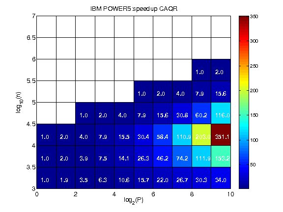
(a) Speedup CAQR

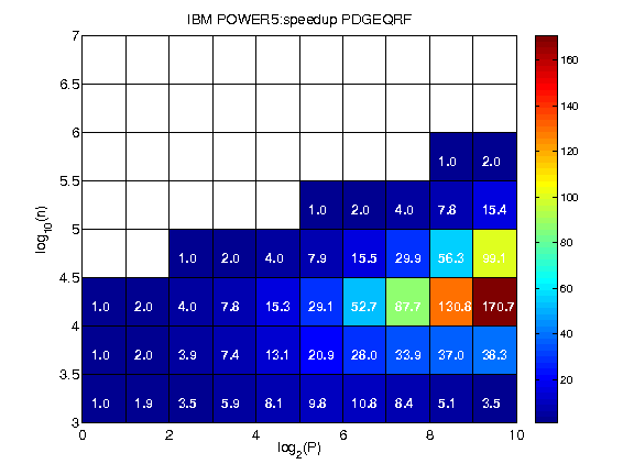
(b) Speedup PDGEQRF

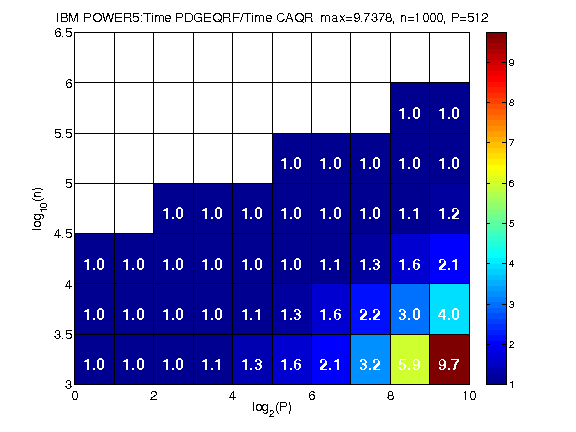
(c) Comparison

Figure 8: Performance prediction comparing CAQR and PDGEQRF on IBM POWER5.

$\log_{10}n$	Best $\log_{2}P$ for PDGEQRF	CAQR speedup
3.0	6	2.1
3.5	8	3.0
4.0	9	2.1
4.5	9	1.2
5.0	9	1.0
5.5	9	1.0

Table 19: Estimated runtime of PDGEQRF divided by estimated runtime of CAQR on a square $n\times n$ matrix, on the IBM POWER5 platform, for those values of $P$ (number of processors) for which PDGEQRF performs the best for that problem size.

(a) Optimal $b$

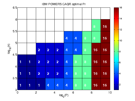
(b) Optimal $P_{r}$

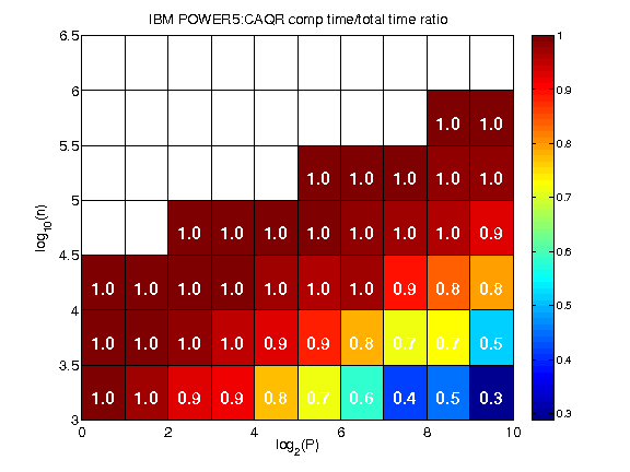
(c) Fraction of time in computation

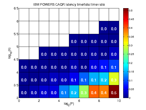
(d) Fraction of time in latency

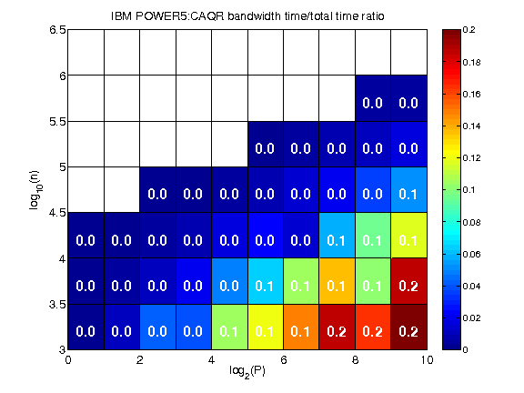
(e) Fraction of time in bandwidth

Figure 9: Performance prediction for CAQR on IBM POWER5.

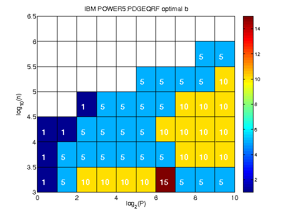
(a) Optimal $b$

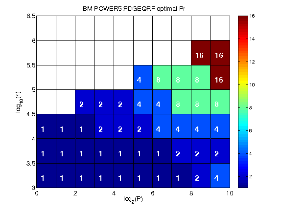
(b) Optimal $P_{r}$

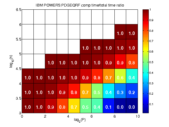
(c) Fraction of time in computation

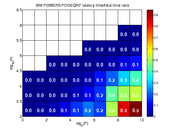
(d) Fraction of time in latency

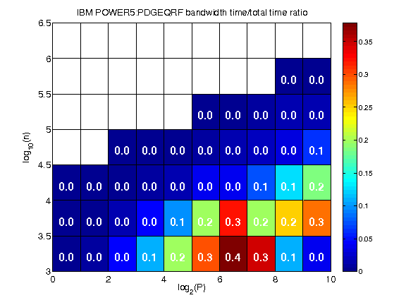
(e) Fraction of time in bandwidth

Figure 10: Performance prediction for PDGEQRF on IBM POWER5.

16.2 Performance prediction on Peta

Figures 11, 12, and 13 show our performance estimates of CAQR and PDGEQRF on the Petascale machine. The estimated division of time between computation, latency, and bandwidth for PDGEQRF is illustrated in Figures 13(c), 13(d), and 13(e). In the upper left corner of these figures, the computation dominates the total time, while in the right bottom corner the latency dominates the total time. In the narrow band between these two regions, which goes from the left bottom corner to the right upper corner, the bandwidth dominates the time. CAQR decreases the latency cost, as can be seen in Figures 12(c), 12(d), and 12(e). There are fewer test cases for which the latency dominates the time (the right bottom corner of Figure 12(d)). This shows that CAQR is expected to be effective in decreasing the latency cost. The left upper region where the computation dominates the time is about the same for both algorithms. Hence for CAQR there are more test cases for which the bandwidth term is an important fraction of the total time.

Note also in Figures 13(b) and 12(b) that optimal $P_{r}$ has smaller values for PDGEQRF than for CAQR. There is an interesting regularity in the value of optimal $P_{r}$ for CAQR. CAQR is expected to have its best performance for (almost) square grids.

As can be seen in Figure 11(a), CAQR is expected to show good scalability for large matrices. For example, for $n=10^{5.5}$, a speedup of $1431$, measured with respect to the time on $2$ processors, is obtained on $8192$ processors. For $n=10^{6.4}$ a speedup of $166$, measured with respect to the time on $32$ processors, is obtained on $8192$ processors.

CAQR leads to more significant improvements when the latency represents an important fraction of the total time. This corresponds to the right bottom corner of Figure 11(c). The best improvement is a factor of $22.9$, obtained for $n=10^{4}$ and $P=8192$. The speedup of the best CAQR compared to the best PDGEQRF for $n=10^{4}$ when using at most $P=8192$ processors is larger than $8$, which is still an important improvement. The best performance of CAQR is obtained for $P=4096$ processors and the best performance of PDGEQRF is obtained for $P=16$ processors.

Useful improvements are also obtained for larger matrices. For $n=10^{6}$, CAQR outperforms PDGEQRF by a factor of $1.4$. When the computation dominates the parallel time, there is no benefit from using CAQR. However, CAQR is never slower. For any fixed $n$, we can take the number of processors $P$ for which PDGEQRF would perform the best, and measure the speedup of CAQR over PDGEQRF using that number of processors. We do this in Table 20, which shows that CAQR always is at least as fast as PDGEQRF, and often significantly faster (up to $7.4\times$ faster in some cases).

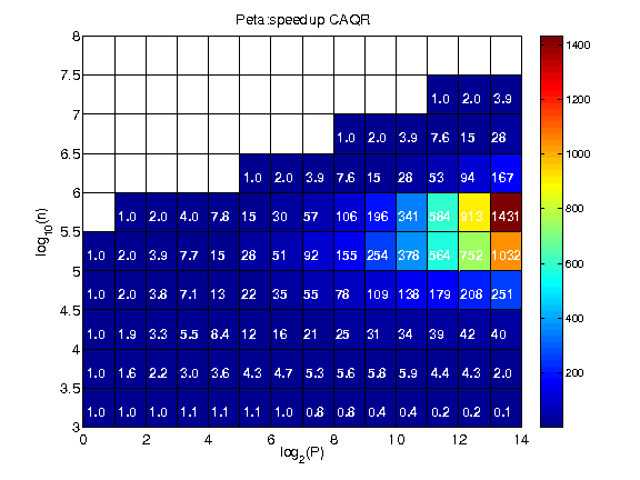
(a) Speedup CAQR

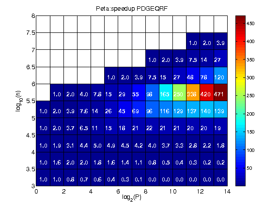
(b) Speedup PDGEQRF

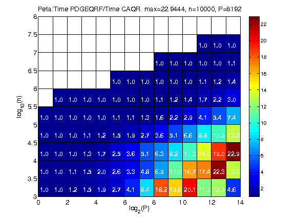
(c) Comparison

Figure 11: Performance prediction comparing CAQR and PDGEQRF on Peta.

$\log_{10}n$	Best $\log_{2}P$ for PDGEQRF	CAQR speedup
3.0	1	1
3.5	2–3	1.1–1.5
4.0	4–5	1.7–2.5
4.5	7–10	2.7–6.6
5.0	11–13	4.1–7.4
5.5	13	3.0
6.0	13	1.4

Table 20: Estimated runtime of PDGEQRF divided by estimated runtime of CAQR on a square $n\times n$ matrix, on the Peta platform, for those values of $P$ (number of processors) for which PDGEQRF performs the best for that problem size.

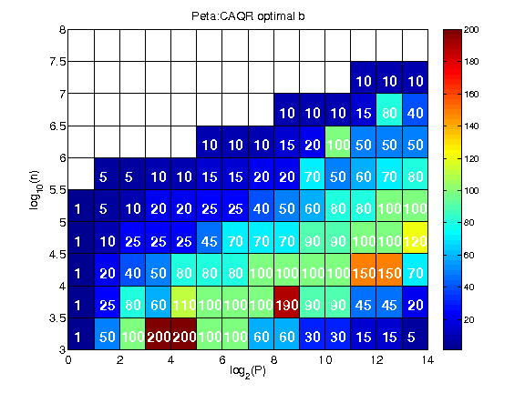
(a) Optimal $b$

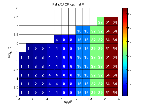
(b) Optimal $P_{r}$

(c) Fraction of time in computation

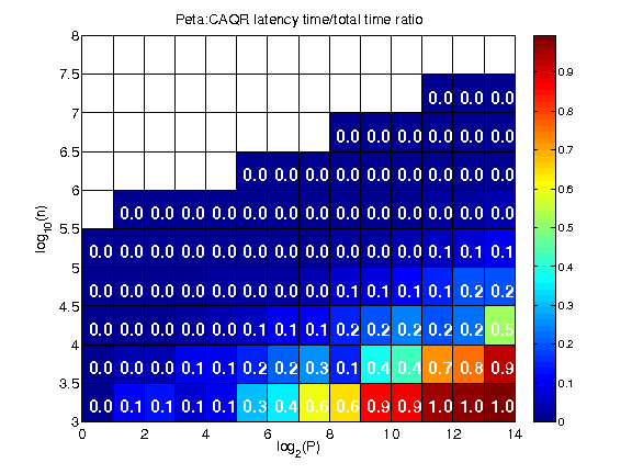
(d) Fraction of time in latency

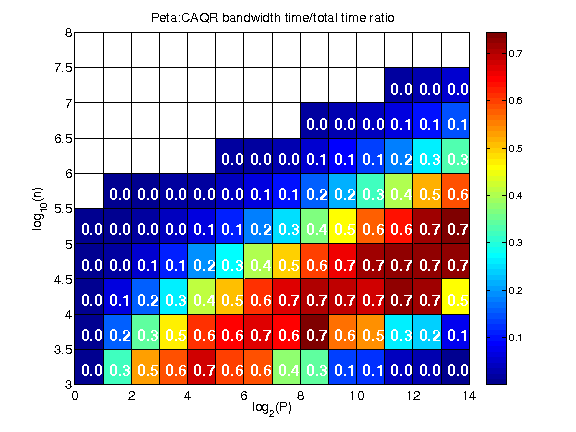
(e) Fraction of time in bandwidth

Figure 12: Performance prediction for CAQR on Peta.

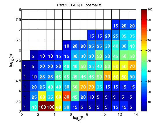
(a) Optimal $b$

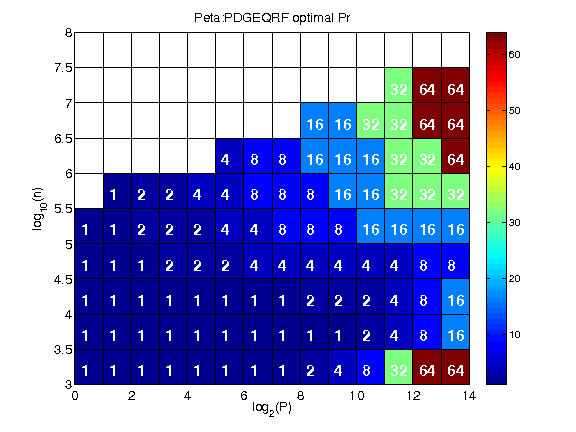
(b) Optimal $P_{r}$

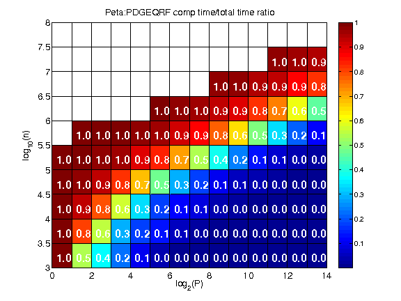
(c) Fraction of time in computation

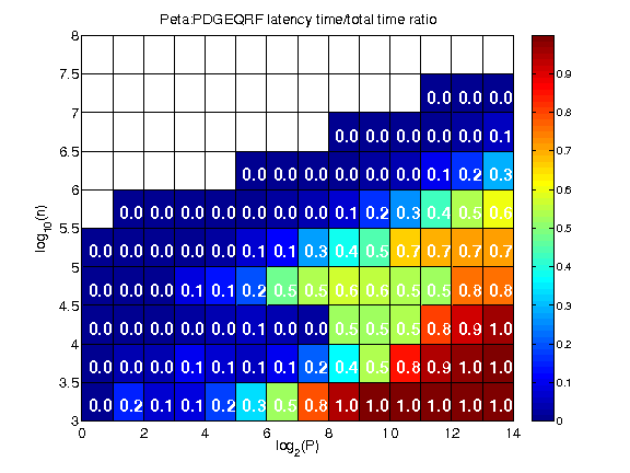
(d) Fraction of time in latency

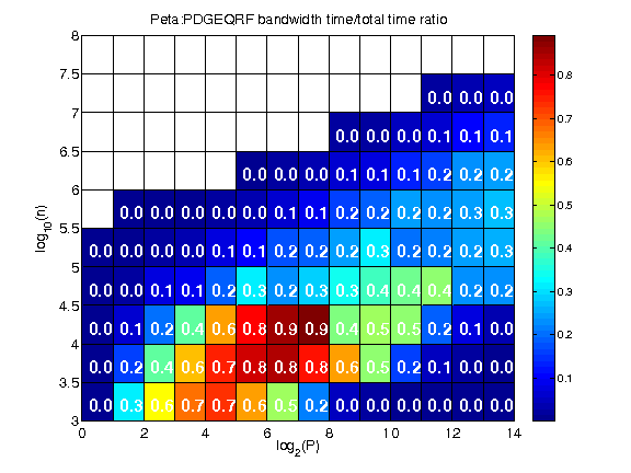
(e) Fraction of time in bandwidth

Figure 13: Performance prediction for PDGEQRF on Peta.

16.3 Performance prediction on Grid

The performance estimation obtained by CAQR and PDGEQRF on the Grid is displayed in Figures 14, 15, and 16. For small values of $n$ both algorithms do not obtain any speedup, even on small number of processors. Hence we discuss performance results for values of $n$ bigger than $10^{5}$.

As displayed in Figures 15(a) and 16(a), the optimal block size for both algorithms is very often $200$, the largest value in the allowed range. The optimal value of $P_{r}$ for PDGEQRF is equal to $1$ for most of the test cases (Figure 16(b)), while CAQR tends to prefer a square grid (Figure 15(b)). This suggests that CAQR can successfully exploit parallelism within block columns, unlike PDGEQRF.

As can be seen in Figures 16(c), 16(d), and 16(e), for small matrices, communication latency dominates the total runtime of PDGEQRF. For large matrices and smaller numbers of processors, computation dominates the runtime. For the test cases situated in the band going from the bottom left corner to the upper right corner, bandwidth costs dominate the runtime. The model of PDGEQRF suggests that the best way to decrease the latency cost with this algorithm is to use, in most test cases, a block column cyclic distribution (the layout obtained when $P_{r}=1$). In this case the bandwidth cost becomes significant.

The division of time between computation, latency, and bandwidth has a similar pattern for CAQR, as shown in Figures 15(c), 15(d), and 15(e). However, unlike PDGEQRF, CAQR has as optimal grid shape a square or almost square grid of processors, which suggests that CAQR is more scalable.

The best improvement is obtained for one of the largest matrix in our test set $m=n=10^{6.5}$, where CAQR outperforms PDGEQRF by a factor of $5.3$ on $128$ processors. The speedup obtained by the best CAQR compared to the best PDGEQRF is larger than $4$, and the best performance is obtained by CAQR on $128$ processors, while the best performance of PDGEQRF is obtained on $32$ processors.

CAQR is predicted to obtain reasonable speedups for large problems on the Grid, as displayed in Figure 14(a). For example, for $n=10^{7}$ we note a speedup of $33.4$ on $128$ processors measured with respect to $2$ processors. This represents an improvement of $1.6$ over PDGEQRF. For the largest matrix in the test set, $n=10^{7.5}$, we note a speedup of $6.6$ on $128$ processors, measured with respect to $16$ processors. This is an improvement of $3.8$ with respect to PDGEQRF.

As with the last model, for any fixed $n$, we can take the number of processors $P$ for which PDGEQRF would perform the best, and measure the speedup of CAQR over PDGEQRF using that number of processors. We do this in Table 21, which shows that CAQR always is at least as fast as PDGEQRF, and often significantly faster (up to $3.8\times$ faster in some cases).

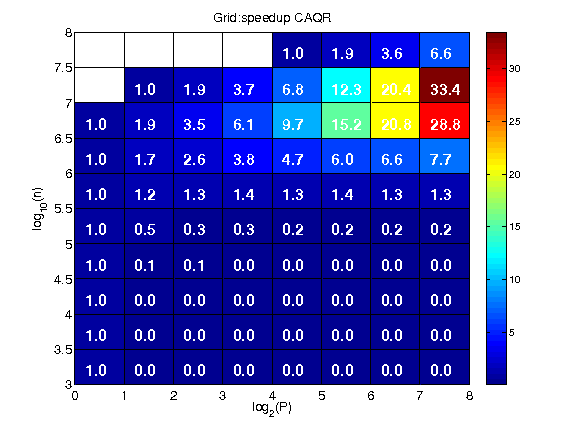
(a) Speedup CAQR

(b) Speedup PDGEQRF

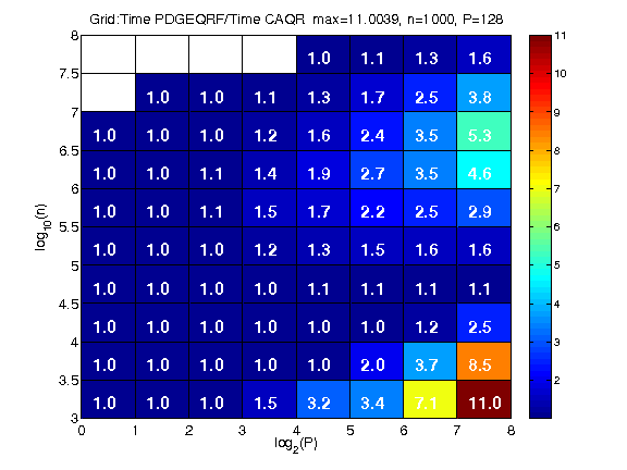
(c) Comparison

Figure 14: Performance prediction comparing CAQR and PDGEQRF on Grid.

$\log_{10}n$	Best $\log_{2}P$ for PDGEQRF	CAQR speedup
6.0	3	1.4
6.5	5	2.4
7.0	7	3.8
7.5	7	1.6

Table 21: Estimated runtime of PDGEQRF divided by estimated runtime of CAQR on a square $n\times n$ matrix, on the Grid platform, for those values of $P$ (number of processors) for which PDGEQRF performs the best for that problem size.

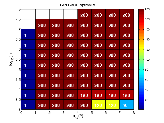
(a) Optimal $b$

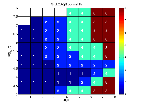
(b) Optimal $P_{r}$

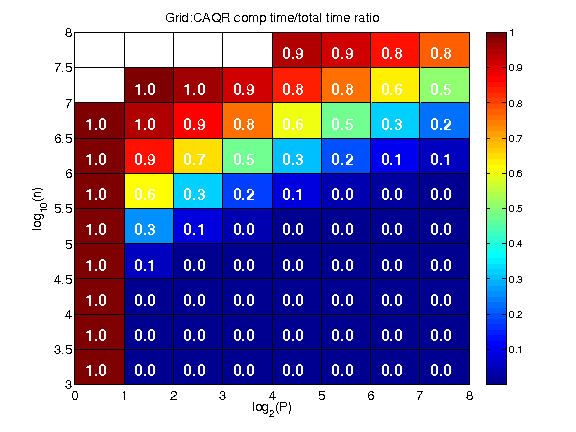
(c) Fraction of time in computation

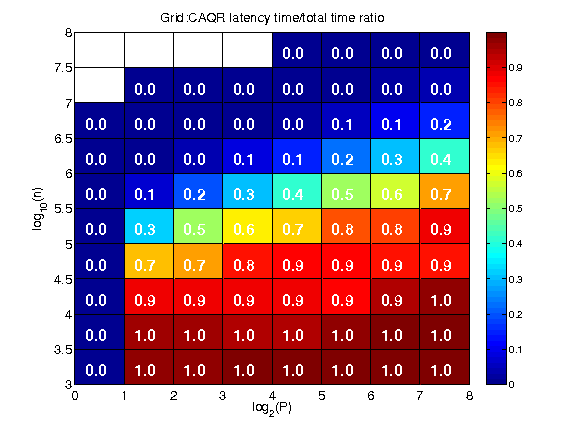
(d) Fraction of time in latency

(e) Fraction of time in bandwidth

Figure 15: Performance prediction for CAQR on Grid.

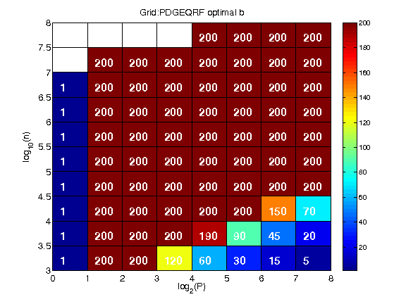
(a) Optimal $b$

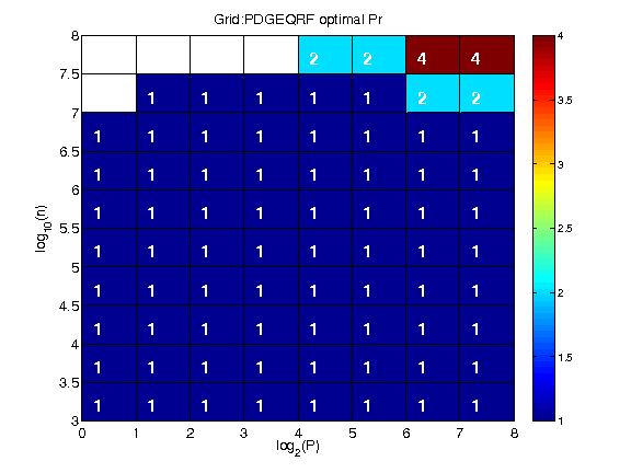
(b) Optimal $P_{r}$

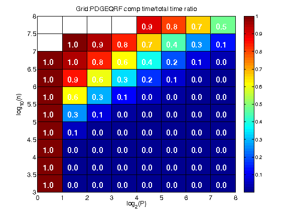
(c) Fraction of time in computation

(d) Fraction of time in latency

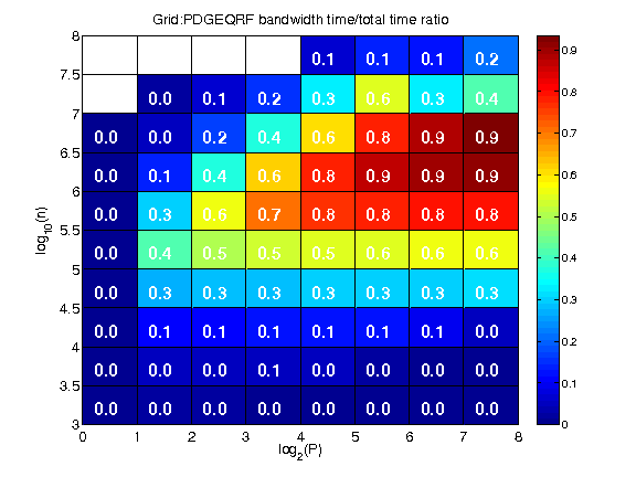
(e) Fraction of time in bandwidth

Figure 16: Performance prediction for PDGEQRF on Grid.

17 Lower bounds on communication for QR

In this section, we review known lower bounds on communication bandwidth for parallel and sequential matrix-matrix multiplication of matrices stored in 1-D and 2-D block cyclic layouts, extend some of them to the rectangular case, and then extend them to QR, showing that our sequential and parallel TSQR and CAQR algorithms have optimal communication complexity with respect to both bandwidth (in a Big-Oh sense, and sometimes modulo polylogarithmic factors).

We will also use the simple fact that if $B$ is a lower bound on the number of words that must be communicated to implement an algorithm, and if $W$ is the size of the local memory (in the parallel case) or fast memory (in the sequential case), so that $W$ is the largest possible size of a message, then $B/W$ is a lower bound on the latency, i.e. the number of messages needed to move $B$ words into or out of the memory. We use this to derive lower bounds on latency, which are also attained by our algorithms (again in a Big-Oh sense, and sometimes modulo polylogarithmic factors).

We begin in section 17.1 by reviewing known communication complexity bounds for matrix multiplication, due first to Hong and Kung [hong1981io] in the sequential case, and later proved more simply and extended to the parallel case by Irony, Toledo and Tiskin [irony2004communication]. It is easy to extend lower bounds for matrix multiplication to lower bounds for LU decomposition via the following reduction of matrix multiplication to LU decomposition:

$$\begin{pmatrix}I&0&-B\\ A&I&0\\ 0&0&I\\ \end{pmatrix}=\begin{pmatrix}I&&\\ A&I&\\ 0&0&I\\ \end{pmatrix}\begin{pmatrix}I&0&-B\\ &I&A\cdot B\\ &&I\\ \end{pmatrix}.$$ (40)

See [grigori2008calu] for an implementation of parallel LU that attains these bounds. It is reasonable to expect that lower bounds for matrix multiplication will also apply (at least in a Big-Oh sense) to other one-sided factorizations, such as QR. Though as we will see, QR is not quite so simple.

All this work assumes commutative and associative reorderings of the conventional $O(n^{3})$ matrix multiplication algorithm, and so excludes faster algorithms using distributivity or special constants, such as those of Strassen [strassen1969gaussian] or Coppersmith and Winograd [coppersmith1982asymptotic], and their use in asymptotically fast versions of LU and QR [FastLinearAlgebraIsStable]. Extending communication lower bounds to these asymptotically faster algorithms is an open problem.

17.1 Matrix Multiplication Lower Bounds

Hong and Kung [hong1981io], and later Irony, Toledo and Tiskin [irony2004communication] considered the multiplication of two $n$-by-$n$ matrices $C=A\cdot B$ using commutative and associative (but not distributive) reorderings of the usual $O(n^{3})$ algorithm.

In the sequential case, they assume that $A$ and $B$ initially reside in slow memory, that there is a fast memory of size $W<n^{2}$, and that the product $C=A\cdot B$ must be computed and eventually reside in slow memory. They bound from below the number of words that need to be moved between slow memory and fast memory to perform this task:

$${\rm\#\ words\ moved}\geq\frac{n^{3}}{2\sqrt{2}W^{1/2}}-W\approx\frac{n^{3}}{2\sqrt{2}W^{1/2}}\;\;.$$ (41)

Since only $W$ words can be moved in one message, this also provides a lower bound on the number of messages:

$${\rm\#\ messages}\geq\frac{n^{3}}{2\sqrt{2}W^{3/2}}-1\approx\frac{n^{3}}{2\sqrt{2}W^{3/2}}\;\;.$$ (42)

In the rectangular case, where $A$ is $n$-by-$r$, $B$ is $r$-by-$m$, and $C$ is $n$-by-$m$, so that the number of arithmetic operations in the standard algorithm is $2mnr$, the above two results still apply, but with $n^{3}$ replaced by $mnr$.

Irony, Toledo and Tiskin also consider the parallel case. There is actually a spectrum of algorithms, from the so-called 2D case, that use little extra memory beyond that needed to store equal fractions of the matrices $A$, $B$ and $C$ (and so about $3n^{2}/P$ words for each of $P$ processors, in the square case), to the 3D case, where each input matrix is replicated up to $P^{1/3}$ times, so with each processor needing memory of size $n^{2}/P^{2/3}$ in the square case. We only consider the 2D case, which is the conventional, memory scalable approach. In the 2D case, with square matrices, Irony et al show that if each processor has $\mu n^{2}/P$ words of local memory, and $P\geq 32\mu^{3}$, then at least one of the processors must send or receive at least the following number of words:

$${\rm\#\ words\ sent\ or\ received}\geq\frac{n^{2}}{4\sqrt{2}(\mu P)^{1/2}}$$ (43)

and so using at least the following number of messages (assuming a maximum message size of $n^{2}/P$):

$${\rm\#\ messages}\geq\frac{P^{1/2}}{4\sqrt{2}(\mu)^{3/2}}\;\;.$$ (44)

We wish to extend this to the case of rectangular matrices. We do this in preparation for analyzing CAQR in the rectangular case. The proof is a simple extension of Thm. 4.1 in [irony2004communication].

Theorem 1

Consider the conventional matrix multiplication algorithm applied to $C=A\cdot B$ where $A$ is $n$-by-$r$, $B$ is $r$-by-$m$, and $C$ is $n$-by-$m$. implemented on a $P$ processor distributed memory parallel computer. Let $\bar{n}$, $\bar{m}$ and $\bar{r}$ be the sorted values of $n$, $m$, and $r$, i.e. $\bar{n}\geq\bar{m}\geq\bar{r}$. Suppose each processor has $3\bar{n}\bar{m}/P$ words of local memory, so that it can fit 3 times as much as $1/P$-th of the largest of the three matrices. Then as long as

$$\bar{r}\geq\sqrt{\frac{864\bar{n}\bar{m}}{P}}$$ (45)

(i.e. none of the matrices is “too rectangular”) then the number of words at least one processor must send or receive is

$${\rm\#\ words\ moved}\geq\frac{\sqrt{\bar{n}\bar{m}}\cdot\bar{r}}{\sqrt{96P}}$$ (46)

and the number of messages is

$${\rm\#\ messages}\geq\frac{\sqrt{P}\cdot\bar{r}}{\sqrt{864\bar{n}\bar{m}}}$$ (47)

Proof: We use (41) with $\bar{m}\bar{n}\bar{r}/P$ substituted for $n^{3}$, since at least one processor does this much arithmetic, and $W=3\bar{n}\bar{m}/P$ words of local memory. The constants in inequality (45) are chosen so that the first term in (41) is at least $2W$, and half the first term is a lower bound. $\Box$

17.2 Lower bounds for TSQR

TSQR with data stored in a 1D layout is simpler than the general CAQR case, and does not depend on the above bounds for matrix multiplication.

17.2.1 Sequential TSQR

In the sequential case, the $m\times n$ matrix $A$ must be read from slow memory into fast memory at least once, if we assume that fast memory is empty at the start of the computation, and the answer written out to slow memory. Thus, the number of words transferred (the bandwidth lower bound) is at least $2mn$. As described in Table 11 in Section 9, and in more detail in Appendix B, our sequential TSQR moves

$$\frac{mn^{2}}{W-n(n+1)/2}+2mn-\frac{n(n+1)}{2}$$

words. Since we assume $W\geq\frac{3}{2}n^{2}$, this is little more than the lower bound $2mn$. In contrast, blocked left-looking Householder QR moves

$$+\frac{m^{2}n^{2}}{2W}-\frac{mn^{3}}{6W}+\frac{3mn}{2}-\frac{3n^{2}}{4}$$

words, where the first and second terms combined can be $O(\frac{mn}{W})$ times larger than the lower bound (see Table 11); note that $\frac{mn}{W}$ is how many times larger the matrix is than the fast memory.

The number of slow memory reads and writes (the latency lower bound) is at least $2mn/W$. As described in the same sections as before, our sequential TSQR sends

$$\frac{2mn}{W-n(n+1)/2}$$

words, which is close to the lower bound. In contrast, blocked left-looking Householder QR sends

$$\frac{2mn}{W}+\frac{mn^{2}}{2W}$$

messages, which can be $O(n)$ times larger than the lower bound (see Table 11).

17.2.2 Parallel TSQR

In the parallel case, we prefer for 1-D layouts to distinguish between the minimum number of messages per processor, and the number of messages along the critical path. For example, one can perform a reduction linearly, so that each processor only sends one message to the next processor. This requires $P-1$ messages along the critical path, but only one message per processor. A lower bound on the minimum number of sends or receives performed by any processor is also a lower bound on the number of messages along the critical path. The latter is more difficult to analyze for 2-D layouts, so we only look at the critical path for 1-D layouts. By the usual argument that any nontrivial function of data distributed across $P$ processors requires at least $\log_{2}P$ messages to compute, the critical path length $C_{\text{1-D}}(m,n,P)$ satisfies

$$C_{\text{1-D}}(m,n,P)\geq\log_{2}P.$$ (48)

This is also the number of messages required per processor along the critical path. This lower bound is obviously attained by parallel TSQR based on a binary tree.

Appendix LABEL:S:CommLowerBoundsFromCalculus shows formally that for any reduction tree computing the QR decomposition of $\frac{m}{p}\times n$ matrices at its leaves, each path from the leaves to the root must send at least $n(n+1)/2$ words of information along each edge. This means the bandwidth cost is at least $n(n+1)/2$ times the length of critical path, or at least $\log(P)n(n+1)/2$. This is clearly attained by TSQR (see Table 10).

17.3 Lower Bounds for CAQR

Now we need to extend our analysis of matrix multiplication. We assume all variables are real; extensions to the complex case are straightforward. Suppose $A=QR$ is $m$-by-$n$, $n$ even, so that

$$\bar{Q}^{T}\cdot\bar{A}\equiv\left(Q(1:m,1:\frac{n}{2})\right)^{T}\cdot A(1:m,\frac{n}{2}+1:n)=R(1:\frac{n}{2},\frac{n}{2}+1:n)\equiv\bar{R}\;\;.$$

It is easy to see that $\bar{Q}$ depends only on the first $\frac{n}{2}$ columns of $A$, and so is independent of $\bar{A}$. The obstacle to directly applying existing lower bounds for matrix multiplication of course is that $\bar{Q}$ is not represented as an explicit matrix, and $\bar{Q}^{T}\cdot\bar{A}$ is not implemented by straightforward matrix multiplication. Nevertheless, we argue that the same data dependencies as in matrix multiplication can be found inside many implementations of $\bar{Q}^{T}\cdot\bar{A}$, and that therefore the geometric ideas underlying the analysis in [irony2004communication] still apply. Namely, there are two data structures $\tilde{Q}$ and $\tilde{A}$ indexed with pairs of subscripts $(j,i)$ and $(j,k)$ respectively with the following properties.

• $\tilde{A}$ stores $\bar{A}$ as well as all intermediate results which may overwrite $\bar{A}$.

• $\tilde{Q}$ represents $\bar{Q}$, i.e., an $m$-by-$\frac{n}{2}$ orthogonal matrix. Such a matrix is a member of the Stiefel manifold of orthogonal matrices, and is known to require $\frac{mn}{2}-\frac{n}{4}(\frac{n}{2}+1)$ independent parameters to represent, with column $i$ requiring $m-i$ parameters, although a particular algorithm may represent $\bar{Q}$ using more data.

• The algorithm operates mathematically independently on each column of $\bar{A}$, i.e., methods like that of Strassen are excluded. This means that the algorithm performs at least $\frac{mn}{2}-\frac{n}{4}(\frac{n}{2}+1)$ multiplications on each $m$-dimensional column vector of $\bar{A}$ (see subsection LABEL:SS:lowerbounds:2d:flops for a proof), and does the same operations on each column of $\bar{A}$.

• For each $(i,k)$ indexing $\bar{R}_{i,k}$, which is the component of the $k$-th column $\bar{A}_{:,k}$ of $\bar{A}$ in the direction of the $i$-th column $\bar{Q}_{:,i}$ of $\bar{Q}$, it is possible to identify at least $m-i$ common components of $\tilde{A}_{:,k}$ and of $\tilde{Q}_{:,i}$ such that a parameter associated with $\tilde{Q}_{j,i}$ is multiplied by a value stored in $\tilde{A}_{j,k}$.

The last point, which says that $\bar{Q}^{T}\cdot\bar{A}$ has at least the same dependencies as matrix multiplication, requires illustration.

• Suppose $\bar{Q}$ is represented as a product of $\frac{n}{2}$ Householder reflections with a projection $\hat{Q}$ onto the first $\frac{n}{2}$ coordinates, $\bar{Q}=(I-\tau_{1}u_{1}u_{1}^{T})\cdots(I-\tau_{n/2}u_{n/2}u_{n/2}^{T})\hat{Q}$, normalized in the conventional way where the topmost nonzero entry of each $u_{j}$ is one, and $\hat{Q}$ consists of the first $n/2$ columns of the $n$-by-$n$ identity matrix. Then $\tilde{Q}_{j,i}=u_{i}(j)$ is multiplied by some intermediate value of $\bar{A}_{j,k}$, i.e. $\tilde{A}_{j,k}$.

• Suppose $\bar{Q}$ is represented as a product of block Householder transformations $(I-Z_{1}U_{1}^{T})\cdots(I-Z_{f}U_{f}^{T})\hat{Q}$ where $U_{g}$ and $Z_{g}$ are $m$-by-$b_{g}$ matrices, $U_{g}$ consisting of $b_{g}$ Householder vectors side-by-side. Again associate $\tilde{Q}_{j,i}$ with the $j$-th entry of the $i$-th Householder vector $u_{i}(j)$.

• Recursive versions of QR [elmroth1998new] apply blocked Householder transformations organized so as to better use BLAS3, but still let us use the approach of the last bullet.

• Suppose $\bar{Q}$ is represented as a product of $\frac{mn}{2}-\frac{n}{4}(\frac{n}{2}+1)$ Givens rotations, each one creating a unique subdiagonal zero entry in $A$ which is never filled in. There are many orders in which these zeros can be created, and possibly many choices of row that each Givens rotation may rotate with to zero out its desired entry. If the desired zero entry in $A_{j,i}$ is created by the rotation in rows $j^{\prime}$ and $j$, $j^{\prime}<j$, then associate $\tilde{Q}_{j,i}$ with the value of the cosine in the Givens rotation, since this will be multiplied by $\bar{A}_{j,k}$.

• Suppose, finally, that we use CAQR to perform the QR decomposition, so that $\bar{Q}=Q_{1}\cdots Q_{f}\hat{Q}$, where each $Q_{g}$ is the result of TSQR on $b_{g}$ columns. Consider without loss of generality $Q_{1}$, which operates on the first $b_{1}$ columns of $A$. We argue that TSQR still produces $m-i$ parameters associated with column $i$ as the above methods. Suppose there are $P$ row blocks, each of dimension $\frac{m}{P}$-by-$b_{1}$. Parallel TSQR initially does QR independently on each block, using any of the above methods; we associate multipliers as above with the subdiagonal entries in each block. Now consider the reduction tree that combines $q$ different $b_{1}$-by-$b_{1}$ triangular blocks at any particular node. As described in subsection 6.1, this generates $(q-1)b_{1}(b_{1}+1)/2$ parameters that multiply the equal number of entries of the $q-1$ triangles being zeroed out, and so can be associated with appropriate entries of $\tilde{Q}$. Following the reduction tree, we see that parallel TSQR produces exactly as many parameters as Householder reduction, and that these may be associated one-for-one with all subdiagonal entries of $\tilde{Q}(:,1:b_{1})$ and $\tilde{A}(:,1:b_{1})$ as above. Sequential TSQR reduction is analogous.

We see that we have only tried to capture the dependencies of a fraction of the arithmetic operations performed by various QR implementations; this is all we need for a lower bound.

Now we resort to the geometric approach of [irony2004communication]: Consider a three dimensional block of lattice points, indexed by $(i,j,k)$. Each point on the $(i,0,k)$ face is associated with $\bar{R}_{i,k}$, for $1\leq i,k\leq\frac{n}{2}$. Each point on the $(0,j,k)$ face is associated with $\tilde{A}_{j,k}$, for $1\leq k\leq\frac{n}{2}$ and $1\leq j\leq m$. Each point on the $(i,j,0)$ face is associated with $\tilde{Q}_{j,i}$, for $1\leq i\leq\frac{n}{2}$ and $1\leq j\leq m$. Finally, each interior point $(i,j,k)$ for $1\leq i,k\leq\frac{n}{2}$ and $1\leq j\leq m$ represents the multiplication $\tilde{Q}_{j,i}\cdot\tilde{A}_{j,k}$. The point is that the multiplication at $(i,j,k)$ cannot occur unless $\tilde{Q}_{j,i}$ and $\tilde{A}_{j,k}$ are together in memory.

Finally, we need the Loomis-Whitney inequality [loomis1949inequality]: Suppose $V$ is a set of lattice points in 3D, $V_{i}$ is projection of $V$ along $i$ onto the $(j,k)$ plane, and similarly for $V_{j}$ and $V_{k}$. Let $|V|$ denote the cardinality of $V$, i.e. counting lattice points. Then $|V|^{2}\leq|V_{i}|\cdot|V_{j}|\cdot|V_{k}|$.

Finally, we can state