The weak magnetic field of the O9.7 supergiant $\zeta$ Orionis A

Abstract

We report here the detection of a weak magnetic field of 50–100 G on the O9.7 supergiant $\zeta$ Ori A, using spectropolarimetric observations obtained with NARVAL at the 2m Télescope Bernard Lyot atop Pic du Midi (France). $\zeta$ Ori A is the third O star known to host a magnetic field (along with $\theta^{1}$ Ori C and HD 191612), and the first detection on a ’normal’ rapidly-rotating O star. The magnetic field of $\zeta$ Ori A is the weakest magnetic field ever detected on a massive star. The measured field is lower than the thermal equipartition limit (about 100 G). By fitting NLTE model atmospheres to our spectra, we determined that $\zeta$ Ori A is a 40 ${\rm M}_{\odot}$ star with a radius of 25 ${\rm R}_{\odot}$and an age of about 5–6 Myr, showing no surface nitrogen enhancement and losing mass at a rate of about 2$\times 10^{-6}$ ${\rm M}_{\odot}$ yr^-1.

The magnetic topology of $\zeta$ Ori A is apparently more complex than a dipole and involves two main magnetic polarities located on both sides of the same hemisphere; our data also suggest that $\zeta$ Ori A rotates in about 7.0 d and is about 40^∘ away from pole-on to an Earth-based observer. Despite its weakness, the detected magnetic field significantly affects the wind structure; the corresponding Alfvén radius is however very close to the surface, thus generating a different rotational modulation in wind lines than that reported on the two other known magnetic O stars.

The rapid rotation of $\zeta$ Ori A with respect to $\theta^{1}$ Ori C appears as a surprise, both stars having similar unsigned magnetic fluxes (once rescaled to the same radius); it may suggest that the sub-equipartition field detected on $\zeta$ Ori A is not a fossil remnant (as opposed to that of $\theta^{1}$ Ori C and HD 191612), but the result of an exotic dynamo action produced through MHD instabilities.

1 Introduction

Stellar magnetic fields have been detected across a large range of spectral types. In solar-type and essentially all cool, low-mass (i.e., mid F and later) stars, magnetic fields (and activity) are observed, often featuring a complex topology, and are thought to be due to dynamo processes occuring within the outer convective layers. In hotter, more massive stars with outer radiative zones, magnetic fields are also detected (with a significantly simpler topology though) but only in a small fraction of stars (e.g., the magnetic chemically peculiar stars among the A and late B stars). The situation might be similar (though less well studied) among early B and O stars, with only two O stars (namely $\theta^{1}$ Ori C and HD 191612, Donati et al. 2002, 2006) and less than a handfull of early B-type stars (e.g., $\tau$ Sco, $\beta$ Cep, $\zeta$ Cas, Donati et al. 2006, 2001; Neiner et al. 2003) yet known as magnetic.

Magnetic fields are nonetheless expected to play a significant role throughout the evolution of hot massive stars, by modifying the internal rotation, enhancing chemical transport and mixing, and producing enhanced surface abundances (Maeder & Meynet, 2003, 2004, 2005). Magnetic fields can also dramatically influence the way winds are launched (e.g., ud-Doula & Owocki, 2002) and the later phases of evolution (e.g., the collapse, Heger et al., 2005); a large number of observational phenomena (e.g., non-thermal radio emission, anomalous X-ray spectra, abundance anomalies, and H$\alpha$ modulation) can also be explained (qualitatively at least) by the existence of a weak magnetic field. Yet, the origin of magnetism in massive stars is still an open question, with a lively debate between two classes of models. While some models assert that dynamo processes (either located in the convective core, e.g., Charbonneau & MacGregor 2001, or acting within the radiative zone, e.g., Mullan & MacDonald 2005) can produce the observed magnetic fields, some others claim that the field is fossil in nature (Ferrario & Wickramasinghe, 2005, 2006), being advected and amplified through the initial protostellar collapse.

The limited knowledge that we have about the existence and statistical properties of magnetic fields in massive O stars is mostly due to the fact that these fields are difficult to detect. Absorption lines of O stars are both relatively few in number in the optical domain, and generally rather broad (because of rotation or to some other type of as yet unknown macroscopic mechanism, e.g., Howarth et al. 1997), decreasing dramatically the size of the Zeeman signatures that their putative fields can induce. The results obtained so far (on two stars only) suggest that magnetic O-type stars may be (i) slow rotators and (ii) may exhibit a peculiar spectrum with very regular temporal modulation. While this view may partly reflect an observational bias (magnetic detections being easier on slow rotators) or a selection effect (observations often concentrating on peculiar stars first), null results recently reported on intermediate and fast rotators argue that this effect may be real. This question is nevertheless a key point for clarifying both the origin and evolutionary impact of magnetic fields in massive stars and therefore deserves being studied with great care.

With the advent of the new generation spectropolarimeters, such as ESPaDOnS at the Canada-France-Hawaii Telescope (CFHT) in Hawaii and NARVAL on the Télescope Bernard Lyot (TBL) in southern France, studies of stellar magnetic fields have undergone a big surge of activity; in particular, detecting magnetic fields of massive O stars (or providing upper limits of no more than a few tens of G) is now within reach. In this context, we recently initiated a search for magnetic fields in a limited number of ’normal’ O stars, using NARVAL.

One of our targets is $\zeta$ Ori A, a O9.7 Ib supergiant (Maíz-Apellániz et al., 2004) and the brightest O star at optical wavelengths. Evidence for azimuthal wind structuration (with an modulation timescale of about 6 d, compatible with the rotation period) is reported from both UV and optical lines (e.g., Kaper et al., 1996, 1999) and possibly due to the presence of a weak magnetic field. $\zeta$ Ori A is also well-known for its prominent X-ray emission, $\hbox{$\log L_{\rm X}/L_{\rm bol}$}=-6.74$ (Berghoefer et al., 1997). The origin of this X-ray emission is however still controversial; while Cohen et al. (2006) suggest that it is due to the classical wind-shock mechanism (with X-rays originating from cooling shocks in the acceleration zone), Raassen et al. (2008) invoke a collisional ionization equilibrium model and Pollock (2007) argue for collisionless shocks controlled by magnetic fields in the wind terminal velocity regime. For all these reasons, $\zeta$ Ori A is an obvious candidate for our magnetic exploration program.

In this paper, we report our spectropolarimetric observations of $\zeta$ Ori A and present the Zeeman detections we obtained (Sec. 2). From the collected spectra, we reexamine the fundamental parameters of $\zeta$ Ori A and discuss the observed rotational modulation to attempt pinning down the rotation period (Sec. 3). We then carry out a complete modeling of the detected Zeeman signatures and describe the reconstructed magnetic topology (Sec. 4). We finally summarise our results, discuss their implications for our understanding of massive magnetic stars, and suggest new observations to confirm and expand our conclusions (Sec. 5).

2 Observations

Spectropolarimetric observations of $\zeta$ Ori A were collected with NARVAL at TBL in 2007 October, as part of a 10-night run aimed at investigating the magnetic fields of hot stars. $\zeta$ Ori A was observed during seven nights; altogether, 292 circular-polarization sequences, each consisting of four individual subexposures taken in different polarimeter configurations, were obtained. From each set of four subexposures we derive a mean Stokes $V$ spectrum following the procedure of Donati et al. (1997), ensuring in particular that all spurious signatures are removed at first order. Null polarisation spectra (labelled $N$) are calculated by combining the four subexposures in such a way that polarization cancels out, allowing us to check that no spurious signals are present in the data (Donati et al. 1997, see for more details on how $N$ is defined). All frames were processed using Libre ESpRIT (Donati et al. 1997; Donati et al., in prep.), a fully automatic reduction package installed at TBL for optimal extraction of NARVAL spectra. The peak signal-to-noise ratios per 2.6 km s^-1 velocity bin range from 800 to 1500, depending mostly on weather conditions (see Table 1).

Table 1: Journal of observations. Columns 1–5 list the date, the range of heliocentric Julian dates, the range of UT times, the number of sequences and the exposure time per individual sequence subexposure, and the range of peak signal to noise ratio (per 2.6 km s^-1 velocity bin), for each night of observation. Column 6 lists the rms noise level (relative to the unpolarized continuum level and per 7.2 km s^-1 velocity bin) in the circular polarization profile produced by Least-Squares Deconvolution once averaged over the whole night (Section 2). The rotation cycle (using the ephemeris given by Eq. 1) is listed in column 7.

Date	HJD	UT	$t_{\rm exp}$	S/N	$\sigma_{\rm LSD}$	Phase
(2007)	(2,454,000+)	(h:m:s)	(s)		($10^{-4}I_{\rm c}$)
Oct. 18	391.53928–391.69519	00:52:56–04:37:25	$48\times 4\times 20$	780– 990	0.41	0.648–0.670
Oct. 19	392.69363–392.72343	04:35:04–05:17:59	$8\times 4\times 40$	1010–1080	0.87	0.813–0.817
Oct. 20	393.54410–393.72674	00:59:39–05:22:38	$44\times 4\times 40$	1220–1470	0.28	0.935–0.961
Oct. 21	394.46543–394.66510	23:06:15–03:53:46	$48\times 4\times 40$	810–1460	0.28	1.066–1.095
Oct. 22	395.49302–395.69959	23:45:52–04:43:19	$48\times 4\times 40$	1090–1480	0.27	1.213–1.242
Oct. 24	397.47086–397.67036	23:13:45–04:01:01	$48\times 4\times 40$	1030–1480	0.27	1.495–1.524
Oct. 25	398.50205–398.70310	23:58:34–04:48:03	$48\times 4\times 40$	1200–1470	0.27	1.643–1.671

Least-Squares Deconvolution (LSD; Donati et al. 1997) was applied to all observations. The line list was constructed manually to include the few moderate to strong absorption lines that are not (or only weakly) affected by the wind. The strong Balmer lines, all showing clear emission from the wind and/or circumstellar environment at the time of our observations, were also excluded from the list. The C iv lines at 580.13 and 581.20 nm are used as reference photospheric lines from which we obtain the average radial velocity of $\zeta$ Ori A (about 45 km s^-1); a few unblended absorption lines that are not blueshifted with respect to the reference frame by more than 15 km s^-1 are also included in the list. We end up with a list of only six lines, whose characteristics are summarised in Table 2.

Table 2: Lines used for Least-Squares Deconvolution. The line depths (column 3) were directly measured from our spectra while the Landé factors (column 4) were derived assuming LS coupling.

Wavelength	Element	Depth	Landé
(nm)		($I_{\rm c}$)	factor
492.1931	He i	0.44	1.000
501.5678	He i	0.37	1.000
541.1516	He ii	0.35	1.000
559.2252	O iii	0.40	1.000
580.1313	C iv	0.20	1.167
581.1970	C iv	0.15	1.333

From those lines we produced a mean circular polarization profile (LSD Stokes $V$ profile), a mean check ($N$ for null) profile and a mean unpolarized profile (LSD Stokes $I$ profile) for each spectrum. All LSD profiles were produced on a spectral grid with a velocity bin of 7.2 km s^-1. Averaging together all LSD profiles recorded on each night of the seven nights of observation (with weights proportional to the inverse variance of each profile) yields relative noise levels of 0.27 (in units of $10^{-4}I_{\rm c}$) except on the first two nights (where the noise reaches 0.41 and 0.87). On Oct. 24, the detection probability exceeds 99%, with a reduced-$\chi^{2}$ value (compared to a null-field, $V=0$ profile) of 1.33; the corresponding Stokes $V$ (and null $N$) LSD profiles are shown in Fig. 1. Similar (though less clear) Zeeman signatures are also observed during the other nights.

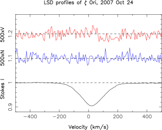
Figure 1: LSD Stokes $V$ (top), null $N$ (middle) and Stokes $I$ profiles of $\zeta$ Ori A on 2007 Oct 24. The $V$ and $N$ profiles are expanded by a factor of 500 and shifted upwards by 1.2 and 1.1 for display purposes. A clear Zeeman signature is detected in the red line wing while the null profile shows no signal.

3 Parameters and rotation of $\zeta$ Ori A

3.1 The photosphere and wind of $\zeta$ Ori A

We reexamine the spectral properties and fundamental parameters of $\zeta$ Ori A, using the new recorded spectra.

We have performed the spectrum analysis using model atmospheres calculated with the unified model code CMFGEN (Hillier & Miller, 1998). CMFGEN provides a consistent treatment of the photosphere and the wind, thus offering useful insights into the wind properties while providing a realistic treatment of photospheric metal-line blanketing. The code solves for the atmospheric structure, non-LTE populations and the radiation field, in the comoving frame of the fluid. The fundamental stellar parameters ($T_{\rm eff}$, $\log g$, $R_{\star}$ and abundances) must be specified at this step, together with the mass-loss rate and velocity law. After convergence of the model, a formal solution of the radiative transfer equation is computed in the observer’s frame, thus providing the synthetic spectrum for comparison to observations. For more details on this code, we refer to Hillier & Miller (1998) and Hillier et al. (2003). CMFGEN does not solve the full hydrodynamics, but rather assumes a density structure. We use a hydrostatic density structure computed with TLUSTY (Hubeny & Lanz, 1995; Lanz & Hubeny, 2003) in the deeper layers, while the wind regime is described with a standard $\beta$-velocity law. The photosphere and the wind are connected below the sonic point at a wind velocity of about 15 km s^-1.

Radiatively driven winds are intrinsically subject to instabilities, resulting in the formation of discrete structures called “clumps”. Both observational evidence and theoretical arguments foster the concept of highly-structured winds (Eversberg et al., 1998; Dessart & Owocki, 2003, 2005). To investigate spectral signatures of clumping in the wind of $\zeta$ Ori A  and its consequences on the derived wind parameters, we have constructed clumped wind models with CMFGEN. A simple, parametric treatment of wind clumping is implemented in CMFGEN, which is expressed by a volume filling factor, $f$. It assumes a void interclump medium and the clumps to be small compared to the photons mean free path. Clumps start to form in the wind at velocities higher than $v_{\rm cl}$. We refer to Hillier et al. (2003) for a detailed description of wind-clumping.

We adopted a value of the clumping filling factor of $f=0.1$. Test models using $f=1$ revealed little change of the H$\alpha$ profile. As for $v_{\rm cl}$ , models with values from 30 (see Bouret et al., 2005) to 400 km s^-1 showed a larger and larger shift of the central absorption component of H$\alpha$ towards shorter wavelengths. The best match was obtained for $v_{\rm cl}\sim 200$ km s^-1.

A depth-independent microturbulent velocity is included in the computation of the atmospheric structure (i.e., temperature structure & population of individual levels). We chose a value of 5 km s^-1 as the default value (see Martins et al., 2002). For the computation of the detailed spectrum resulting from a formal solution of the radiative transfer equation (i.e., with the populations kept fixed), a depth dependent microturbulent velocity was adopted. In that case, the microturbulent velocity follows the relation $\hbox{$v_{\rm turb}$}(r)=\hbox{$v_{\rm min}$}+(\hbox{$v_{\rm max}$}-\hbox{$v_{\rm min}$})\ v(r)/\hbox{$v_{\infty}$}$ where $v_{\rm min}$ and $v_{\rm max}$ are the minimum and maximum microturbulent velocities, and $v_{\infty}$ the terminal wind velocity. In this formulation, $v_{\rm min}$ is technically equivalent to $\xi_{t}$, the microturbulence in the photosphere. We considered several values of $v_{\rm min}$, searching for consistent fits for the photospheric lines. This is obtained for $\hbox{$v_{\rm min}$}=10$ km s^-1 in the photosphere. $\hbox{$v_{\rm max}$}=0.1\ \hbox{$v_{\infty}$}$ was adopted at the top of the atmosphere.

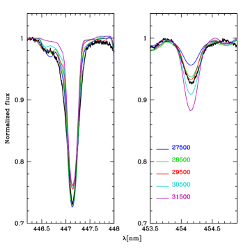
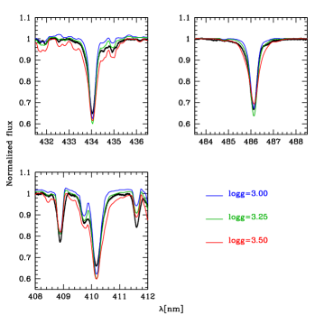
Figure 2: Modeling the 447 nm He i and the 454 nm He ii lines with atmospheric models corresponding to different $T_{\rm eff}$ values (2 left panels; $\log g$ = 3.25), and the H$\delta$, H$\beta$ and H$\epsilon$ lines with models corresponding to different $\log g$ values (3 right panels; $T_{\rm eff}$ = 29,500 K). For this plot, we built a mean spectrum out of the spectra obtained on the night of October 18, 2007.

The effective temperature $T_{\rm eff}$ was derived from the ratio of He ii to He i lines as usually done for O stars. Comparing with models from 27,500 to 31,500 K with 1,000 K steps, we find that $\hbox{$T_{\rm eff}$}=29,500$ K provides the best fit (see Fig. 2). Given the high quality of the observed spectrum, we can clearly exclude the 27,500 and 31,500 K models. Models at 28,500 and 30,500 K already show significant deviations with respect to the best fit. We thus (conservatively) conclude that our estimate is accurate to $\pm$1,000K. The luminosity was derived from the observed magnitude. $\zeta$ Ori A has $m_{\rm V}=1.76$ and $m_{\rm B}=1.59$ (Maíz-Apellániz et al., 2004), which for an intrinsinc color index (B-V)₀ of $-0.26$ (Martins & Plez, 2006), corresponds to an extinction A${}_{\rm V}=0.28$ mag (assuming R_V=3.1). We assumed that the distance to Orion is equal to $d=414\pm 50$ pc (the uncertainty being taken as the dispersion among the various recent measurements published in the literature, Menten et al., 2007). The luminosity of $\zeta$ Ori A can thus be estimated from $m_{\rm V}$, A_V, $d$ and the bolometric correction (equal to $-2.73$ for $\hbox{$T_{\rm eff}$}=29,500$ K, Martins & Plez 2006). We end up with $L=10^{5.64}$ $L_{\odot}$. Combining the uncertainty in $T_{\rm eff}$and $d$ leads to an uncertainty of about 0.15 dex for $L$. The corresponding radius is thus $R=25\pm 5$ ${\rm R}_{\odot}$. We also derived $\log g$ from the shape of H$\beta$, H$\delta$ and H$\epsilon$. We computed models with $\log g$ ranging from 3.0 to 3.75 with 0.25 dex steps. For the three lines, the best match is obtained for $\log g$ = 3.25. The quantification of the goodness of the fit by means of $\chi^{2}$ indicates that the uncertainty is of about 0.1 dex. From the estimates of $\log g$ and $R$, one gets $M=40\pm 20$ ${\rm M}_{\odot}$.

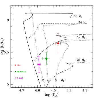
Figure 3: HR diagram with the position of $\zeta$ Ori A, $\theta^{1}$ Ori C and HD 191612 indicated. Parameters for the last two stars are from Simón-Díaz et al. (2006) and Walborn et al. (2003) respectively. Evolutionary tracks are from Meynet & Maeder (2003).

In Fig. 3, we show the position of $\zeta$ Ori A in the HR diagram. The two other known magnetic O stars ($\theta^{1}$ Ori C and HD 191612) are also reported for comparison. We derive an age of 5–6 Myr for $\zeta$ Ori A from the Geneva evolutionary tracks (Meynet & Maeder, 2003). A simple linear interpolation between the evolutionary tracks gives a mass of 39$\pm$8 ${\rm M}_{\odot}$, in good agreement with (and more accurate than) the spectroscopic mass derived above. At first glance, $\zeta$ Ori A thus appears as an evolved couterpart of both $\theta^{1}$ Ori C and HD 191612.

Abundances of a few elements can also be derived. Fig. 4 shows such determinations for CNO, i.e., the most important elements to constrain stellar evolution models. These models predict mixing of CNO-processed material to be more efficient in fast-rotating stars; accordingly, these stars reveal larger CNO surface abundance anomalies at an earlier stage. For instance, Meynet & Maeder (2003) predict for a solar-composition, 40 ${\rm M}_{\odot}$  star with an age of 5 Myr that CNO surface abundances should be equal respectively to 0.5, 5 and 0.6 times their original values. Fig. 4 clearly shows that we do not observe the large N enrichment. The observed N iii lines are best matched with an abundance close to the value found in the Orion nebula (Esteban et al., 2004) and in Orion main-sequence B stars (Cunha & Lambert, 1994). Fitting C iii lines gives uneven results: while some lines are better fitted with the Orion nebula abundance, others indicate a small depletion. Finally, most (but not all) O ii lines indicate that O is underabundant by a factor $\simeq$2. The solar composition assumed for all other elements give good fits to the observed spectrum (e.g., the 448.0 nm Mg ii and the various Si iii and Si iv lines).

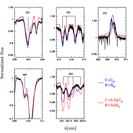
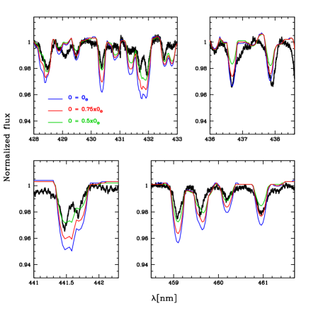
Figure 4: Determining the CN (top) and O (bottom) abundances of $\zeta$ Ori A. In the top panels, the synthetic spectrum corresponding to CN abundances expected for a 40 ${\rm M}_{\odot}$ star at an age of 5 Myr (according to the evolutionary tracks of Meynet & Maeder 2003) is shown in red. In the bottom panels, synthetic spectra with O ii lines are shown for models with O = 0.5, 0.75 and 1.0$~{}\rm{O}_{\odot}$ (evolutionary models predicting O = 0.65$~{}\rm{O}_{\odot}$ at 5 Myr). For this plot, we built a mean spectrum out of the spectra obtained on the night of October 18, 2007.

We used archival IUE spectra to measure the wind terminal velocity from the blueward extension of the strong UV P-Cygni profiles and found $\hbox{$v_{\infty}$}=2,100$ km s^-1. To estimate the mass loss rate, we relied on $H{\alpha}$ only. As $H{\alpha}$ is varying with time (see below), we tried to fit the two profiles respectively featuring the strongest and weakest emission in the far wings (i.e., the part of the profile that can be most reliably fitted with our 1D wind model) to derive the range of $\dot{M}$ over the rotation cycle, yielding values of $\hbox{$\dot{M}$}=1.4-1.9\times 10^{-6}$ ${\rm M}_{\odot}$ yr^-1 (see Fig. 5). We achieved a better match to H$\alpha$ adopting a fast velocity law with $\beta=0.8$. Fitting the position of H$\alpha$ central absorption requires that clumping starts rather high in the wind (at velocities of about 200 km/s). This is larger than what Bouret et al. (2005) found for early O supergiants. A summary of our results from this spectroscopic analysis is presented in Table 3.

Figure 5: Estimating mass loss from H$\alpha$ profiles featuring weakest (left) and strongest (right) emission in the far wings, over our 7d campaign. Matching the broad profile wings yields mass loss rates in the range 1.4–1.9$\times 10^{-6}$ ${\rm M}_{\odot}$ yr^-1. The two weak lines in the red wing are from C ii.

Previous determinations of the physical properties of $\zeta$ Ori A were made by Lamers & Leitherer (1993). They gave $\hbox{$T_{\rm eff}$}=30,900$ K, but this estimate was actually based on the effective temperature scale of Chlebowski & Garmany (1991) and not from a direct analysis of the star with atmospheric models; our finding that $\hbox{$T_{\rm eff}$}=29,500$ K can thus be regarded as a significant improvement with respect to Lamers & Leitherer (1993). In the same study, the luminosity of $\zeta$ Ori A is estimated to $L=10^{5.9}$ $L_{\odot}$, as a result of the larger distance they assumed (500 pc) and to a larger $T_{\rm eff}$ (and thus a larger bolometric correction). Again, our estimate is more robust.

Concerning the abundance patterns, Raassen et al. (2008) recently derived solar C and N content as well as a small O depletion from X-ray spectra. This is consistent with our measurements for these elements. In particular, their data reveal the absence of strong N enrichment. They also report minor Mg and Si enrichment, but this is not confirmed by our results. Finally, Lamers & Leitherer (1993) derived a mass loss rate of $2.5\times 10^{-6}$ ${\rm M}_{\odot}$ yr^-1 from radio measurements; scaled to a distance of 414 pc (they assumed 500 pc), this corresponds to $\hbox{$\dot{M}$}=1.9\times 10^{-6}$ ${\rm M}_{\odot}$ yr^-1, in good agreement with our determination. We set an upper limit to the actual mass-loss rate of $\zeta$ Ori A by searching for the model such that the overall H$\alpha$ profile reaches the peak intensity of the strongest observed H$\alpha$ emission (corresponding to phase 1.082). We find that $\dot{M}$ $<2.5\times 10^{-6}$ ${\rm M}_{\odot}$ yr^-1 (note that the synthetic profile then strongly overestimates the wings strength). We refer to Sec. 5 for a discussion of the origin of the H$\alpha$ emission peak. Note finally that Lamers & Leitherer (1993) value assumes no wind-clumping ($f=1$), while we adopt $f=0.1$ for the optical study.

Table 3: Summary of stellar properties of $\zeta$ Ori A, including photospheric and wind parameters derived from the modeling with CMFGEN. Abundances are expressed relative to Hydrogen. See text for a discussion of the photospheric abundance patterns relative to the initial/local content.

Spectral Type	O9.7 Ib
Distance [pc]	414. $\pm 50$
Rotation period [d]	7.0 $\pm 0.5$
$v\sin i$ [km s-1]	110. $\pm 10$
$v_{mac}$ [km s-1]	93. $\pm 9$
Inclination angle $i$ [∘]	40.
$T_{\rm eff}$ [K]	29,500 $\pm 1000$
$\log g$ [cgs]	3.25 $\pm 0.1$
log $L$ [$L_{\odot}$]	5.64 $\pm 0.15$
M⋆ [M⊙]	40. $\pm 20$
$\xi_{\rm t}$ [km s-1]	10.
$\dot{M}$ [$\times 10^{-6}$ ${\rm M}_{\odot}$ yr-1]	1.4 – 1.9
$v_{\infty}$ [km s-1]	2100.
$\beta$	0.8
$f$	0.1 (default)
$v_{\rm cl}$  [km s-1]	200.
vrad [km s-1]	45. $\pm 5$
$y=$He/H	0.1
C/H	$2.4\pm 0.8\times 10^{-4}$
N/H	$6.0\pm 1.8\times 10^{-5}$
O/H	$4.6\pm 1.4\times 10^{-4}$

3.2 Temporal variability and rotation

Through the Fourier transform of the 580 and 581 nm C iv and O iii 559 nm line profiles (averaged over all lines and nights), we can obtain an accurate estimate of the rotational broadening parameter $v\sin(i)$ (by matching the position of the first zero in the Fourier profile, when this first zero is visible), and of the additional macroscopic turbulent velocity broadening lines (often far) beyond their rotation profiles (e.g. Gray, 1981). We find $v\sin(i)$ $=110\pm 10$ km s^-1(see Fig. 6); for the macroturbulence profile (assumed gaussian), we find $v_{mac}=93\pm 9$ km s^-1(corresponding to a full width at half maximum $110\pm 10$ km s^-1).

Figure 6: Fourier transform of the average 580 and 581 nm C iv and 559 nm O iii line profiles of $\zeta$ Ori A. The full line is obtained from the observed profiles, the dashed line corresponds to the model.

Given the estimated radius (25 ${\rm R}_{\odot}$) and rotational broadening (110 km s^-1) of $\zeta$ Ori A, we conclude that its maximum rotation period $\hbox{$P_{\rm rot}$}/\sin i$ is equal to 11.5 d. Several papers in the refereed literature (e.g., Kaper et al., 1997) mention a possible rotation period (or half-rotation period) of 6 d for $\zeta$ Ori A from variations of Balmer lines. Looking at how Balmer lines evolve with time during our own observations (see Fig. 7, first two left panels) also suggests rotation periods of 6 to 8 d depending on which portion of the line profile we focus on. The central absorption of H$\beta$ and H$\alpha$ (both maximum on Oct 18 and Oct 24, i.e. cycles 0.66 and 1.51) are apparently varying with a timescale of about 6 d, in agreement with the published estimate (e.g., Kaper et al., 1997). The red emission of H$\alpha$ and the red wing of H$\beta$ (minimum on Oct 18 and Oct 25, i.e., cycles 0.66 and 1.66) suggest a slightly longer period. The far blue wing of both Balmer lines shows evidence of excess absorption on Oct 19 and Oct 22 (i.e., cycles 0.82 and 1.23) but not on Oct 25 (cycle 1.66), suggesting a (half) period of about 3.5 d; the far red wing of both lines also show distinct excess absorption on Oct 20 (cycle 0.95). As a matter of fact, we find that variablity is present in a large majority of lines. Most lines exhibit a clear time variable blueshift, maximum on Oct 19 and Oct 24 (cycles 0.8 and 1.5), i.e. on a timescale of at least 4-5d, as showed for the case of He i 492 nm Fig. 7 (third panel from the left). The average blueshift (with respect to C iv 580–581 nm) is $-16$ km s^-1, while the peak-to-peak maximal amplitude is $-17$ km s^-1, well below the radial velocity variations induced by the companion of $\zeta$ Ori A (Hummel et al., 2000).

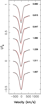
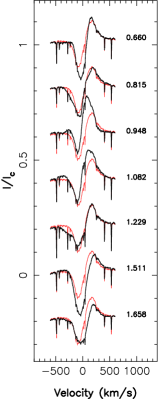
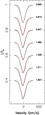
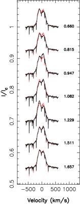
Figure 7: Temporal variations of the H$\beta$ (left), H$\alpha$ (second from left), He i 492 nm (third from left) and 569.59 nm C iii (right) lines throughout our observing run. The time-averaged profile is plotted in red to emphasise variations. The rotational cycle of each observation (assuming a rotation period of 7 d) is written next to each profile. All profiles are shown in the star’s rest frame (i.e., shifted by 45 km s^-1 with respect to the heliocentric rest frame).

We also detect temporal variations in the 569.59 nm C iii double-peak emission line (see Fig. 7, right panel) where the relative intensity of both peaks vary from one night to the next. In our observations, the red peak features maximum emission on Oct 20 and Oct 23 (cycles 0.95 and 1.51) while the blue peak shows maximum emission on Oct 22 (cycle 1.23), apparently in antiphase with the red peak of the same line and in phase with the excess absorption episode occuring in the far blue wing of both Balmer lines. The intensity ratio of both peaks is varying on a timescale of about 3–4 d and may potentially be a good indicator of the rotation half-period.

Given that we detect clear modulation on a period of about 3.5 d both in the far blue wings of both Balmer lines and in emission peak intensity ratio of the C iii line, we interpret the $\simeq$7 d period as the rotation period (rather than half the period as Kaper et al. 1997). The 4-5d timescale seen in most photospheric lines is potentially also compatible with a 7d rotation period (e.g. if the two maximum blueshifts are unevenly spaced in rotation phase).

We therefore assume in the following a 7 d timescale to phase our data, and use the following ephemeris to compute rotational phases:

$$\mbox{HJD}=2454380.0+7.0E.$$ (1)

We further discuss below the determination of the rotation period, using the detected Zeeman signatures to probe rotational modulation. Assuming a rotation period of about 7 d implies that the star is seen at an inclination (with respect to the rotation axis) of about 40^∘, and that the equatorial velocity of $\zeta$ Ori A is about 170 km s^-1. While this is not quite extreme rotation by O star standards, this is already much higher than the two magnetic stars known to date ($\theta^{1}$ Ori C and HD 191612, both featuring equatorial rotation velocities lower than 30 km s^-1).

4 Modelling the magnetic topology of $\zeta$ Ori A

To model the Zeeman signatures of $\zeta$ Ori A, we use the imaging code of Donati et al. (2006). The magnetic topology at the surface of the star is reconstructed as a spherical-harmonic expansion, whose coefficients are adjusted (with a maximum-entropy image reconstruction code) to ensure that the synthetic Zeeman signatures corresponding to the reconstructed magnetic topology match the observed ones at noise level. The magnetic image that we derive can thus be regarded as the simplest topology compatible with the data.

This new imaging method has several advantages with respect to the older one of Brown et al. (1991) and Donati & Brown (1997). The reconstructed field is directly expressed as the sum of a poloidal and a toroidal field. Moreover, we have a direct and obvious way of constraining the degree of complexity of the reconstructed field topology by limiting the spherical harmonic expansion at a given maximum $\ell$ value, depending on the quality and temporal sampling of the available Zeeman data.

For this modeling, we assume that $\hbox{$v\sin(i)$}=110$ km s^-1 and $i=40$^∘, as derived in Sec. 3.2. We also assume that the star and its magnetic topology are rotating as a solid body with a rotation period of 7 d; different values of the rotation period are also used to evaluate how much the result we obtain is sensitive to this parameter (see below). The line profile model (including macroturbulence broadening) used to describe the synthetic Zeeman signatures is the same as that introduced in Sec. 3 to describe the observed photospheric lines, i.e., a simple gaussian at an average wavelength of 500 nm and with full width at half maximum equal to 110 km s^-1. Zeeman signatures are obtained by assuming the weak field approximation and an average Landé factor of 1.1.

The complete set of Zeeman signatures and their corresponding null profiles are shown in Fig. 8 along with the maximum entropy fit to the data, assuming either a simple dipole field or a more complex magnetic geometry (limited to $\ell=3$). The reduced $\chi^{2}_{\nu}$ associated to the global set of $V$ and $N$ profiles with respect to a non magnetic ($B=0$) model are equal to 1.25 and 0.99 respectively (for a total number of 392 data points), indicating that the magnetic signal in the $V$ profiles is unambiguously detected at a 10$\sigma$ level while no significant signal is observed in the $N$ profiles.

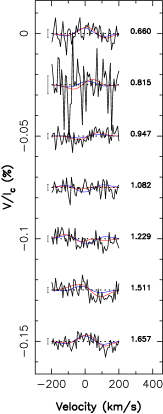
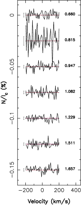
Figure 8: Observed (black) and modeled (red & blue) Stokes $V$ signatures (left) and null $N$ profiles (right) of $\zeta$ Ori A. The blue line corresponds to a simple dipole, while the red one corresponds to a more complex field having $\ell=3$. A clear Zeeman signal is detected and consistently modeled in the Stokes $V$ profiles. The rotational cycle of each observation (assuming a rotation period of 7 d) is written next to each profile. A 1$\sigma$ error bar is also plotted left to each profile.

Assuming that the star hosts a simple dipole field provides a better fit to the data; however, the resulting $\chi^{2}_{\nu}$ (equal to 1.14) is still significantly larger than 1, indicating that the magnetic topology of $\zeta$ Ori A is likely more complex. Using a spherical harmonics series expanded up to $\ell=3$ provides a unit $\chi^{2}_{\nu}$ fit to the data, i.e., is successfull at reproducing the data down to noise level; in particular, it provides a much better fit to the data at cycle 1.51 on the red side (negative dip) of the line profile (see Fig. 8). Unsurprisingly, carrying out the same analysis on the $N$ spectra only yields flat synthetic profiles, the corresponding $\chi^{2}_{\nu}$ for a non-magnetic model being already below 1.

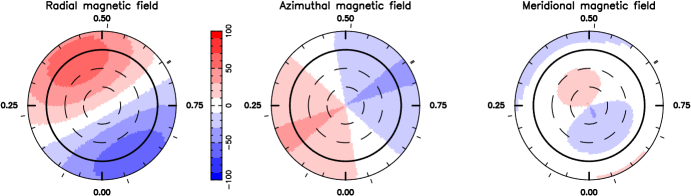
Figure 9: Reconstructed magnetic topology of $\zeta$ Ori A, assuming either a dipole magnetic field (top) or a more complex field having $\ell=3$ (bottom). Only the second (lower) topology provides a $\hbox{$\chi^{2}_{\nu}$}=1$ fit to the Stokes $V$ data. In both cases, the three field components are displayed from left to right (flux values labelled in G). The star is shown in flattened polar projection down to latitudes of $-30\hbox{${}^{\circ}$}$, with the equator depicted as a bold circle and parallels as dashed circles. Radial ticks around each plot indicate phases of observations.

The dipolar and $\ell=3$ magnetic topologies derived from the data are both shown in Fig. 9. The reconstructed dipole has a strength of $61\pm 10$ G, is roughly perpendicular to the rotation axis (inclination angle $\beta=83\pm 10$^∘) with the positive pole facing the observer at phase $0.42\pm 0.03$. The second (more complex) magnetic topology shows more concentrated features (where the field reaches as much 100 G) and is mainly poloidal (the toroidal component containing less than 5% of the reconstructed magnetic energy). Given the limited resolution we have access to on the star (about six resolution elements across the equator given the fairly large width of the local profile), the moderate accuracy to which the Zeeman signatures are detected and the moderate phase coverage of the collected data, there is no real point at carrying out reconstructions with even more complex field topologies.

We carried out the same analysis for different values of the rotation period (and corresponding inclination), looking for the period that produces the magnetic image with the smallest information content and a $\hbox{$\chi^{2}_{\nu}$}=1$ fit to the data. From this process, we derive that 7.5 d is a marginally better rotation period, with a 1$\sigma$ error bar equal to about 0.5 d. The magnetic topologies derived for this value of the rotation period are very similar to those of Fig. 9. Using this criterion, we also find that periods of 12 to 14 d are less likely to be the true rotation period of $\zeta$ Ori A. Note that this constraint on the rotation period depends on the assumed magnetic geometry (here limited to an $\ell\leq 3$ spherical harmonic expansion) given the limited span of our observations (7 d).

5 Discussion

We report in this paper the detection and the first modeling attempt of the weak large-scale magnetic field of the O9.7 supergiant $\zeta$ Ori A. We detect a field that corresponds to local surface magnetic fluxes of only a few tens of G. The field is everywhere lower than 100 G, making it (by far) the weakest magnetic field ever reported in a hot massive star (Donati et al., 1990; Aurière et al., 2007). In particular, this magnetic field is weaker than the thermal equipartition limit, equal to about 100 G for $\zeta$ Ori A; this is the first sub-equipartition field unambiguously detected in a hot star. The magnetic chemically peculiar stars all show fields larger than their thermal equipartition limit (Aurière et al., 2007). This detection also brings the number of known magnetic O stars to three, with $\zeta$ Ori A thus joining $\theta^{1}$ Ori C (Donati et al., 2002) and HD 191612 (Donati et al., 2006). This is also the first magnetic detection in a ’normal’ rapidly rotating O star.

The detailed spectral modeling of $\zeta$ Ori A provides $\hbox{$T_{\rm eff}$}=29,500\pm 1,000$ K and $\hbox{$\log g$}=3.25\pm 0.10$ with normal abundances. It follows that $\zeta$ Ori A is a 40 ${\rm M}_{\odot}$ star with a radius equal to about 25 ${\rm R}_{\odot}$, seen from the Earth at an inclination angle of 40^∘. With an age of about 5–6 Myr, $\zeta$ Ori A essentially appears as an evolved counterpart of both $\theta^{1}$ Ori C and HD 191612. Given its evolutionary stage, $\zeta$ Ori A is expected to show significant N enrichment at its surface (as well as moderate C and O depletion); the normal nitrogen abundance that we measure is thus surprising. It is tempting to suggest that magnetic fields may play a role in this process; this is however not what the first evolutionary models including magnetic field predict (Maeder & Meynet, 2005). More work (both on the observational and theoretical side) are required to investigate this issue further. From a fit to H$\alpha$, we estimate that the mass-loss rate is about 1.4–1.9$\times 10^{-6}$ ${\rm M}_{\odot}$ yr^-1. From the temporal variability of spectral lines and the modulation of Zeeman signatures, we find that the period of $\zeta$ Ori A is about 7d. This is compatible with the $v\sin(i)$ that we measure (from the Fourier shape of the photospheric C iv lines) and the radius that we derive (from the spectral synthesis), provided the star is view at intermediate inclinations ($i=40$ ^∘).

Given that $\zeta$ Ori A is typically 3 and 1.4 times larger in size than $\theta^{1}$ Ori C and HD 191612 respectively, we find that its overall unsigned magnetic flux (i.e., the integral of the absolute value of the magnetic field over stellar surface) is slightly larger (by a factor of about 1.5) than that of $\theta^{1}$ Ori C but much smaller than that of HD 191612 (by about an order of magnitude).

The extremely long rotation period of HD 191612 (about 538 d) suggests that the magnetic field is likely responsible for having dissipated (through confined mass loss) most of the angular momentum of HD 191612 (Donati et al., 2006). The slow rotation rate and extreme youth of $\theta^{1}$ Ori C also suggests that primordial magnetic fields pervading the parent molecular cloud must have a strong impact onto the angular momentum dissipation throughout the cloud collapse, in qualitative agreement with what numerical simulations predict (e.g., Hennebelle & Fromang, 2008). In this context, one would expect $\zeta$ Ori A to rotate, if not as slowly as HD 191612 (whose intrinsic magnetic flux is much higher), at least more slowly than $\theta^{1}$ Ori C (whose intrinsic magnetic flux is similar) given its later evolution stage; this is however not what we observe. No more than speculations can be proposed at this stage. One possibility is that the magnetic field of $\zeta$ Ori A is not of fossil origin (as opposed to that of $\theta^{1}$ Ori C and HD 191612) but rather dynamo generated, making the rotational evolution of $\zeta$ Ori A and $\theta^{1}$ Ori C hardly comparable. The detected magnetic field is indeed much weaker than the critical limit above which MHD instabilities are inhibited (about six times the equipartition field or 600 G in the case of $\zeta$ Ori A, Aurière et al. 2007) and may thus result from exotic dynamo action; the non-dipolar nature of the detected field could be additional evidence in favour of this interpretation, fossil fields being expected to have very simple topologies in evolved stars. Additional spectropolarimetric observations of $\zeta$ Ori A at different epochs (searching for potential variability of the large-scale field) and of similar ’normal’ rapidly-rotating stars are obviously necessary to explore this issue in more details.

Computing the wind magnetic confinement parameter $\eta_{\ast}$ of ud-Doula & Owocki (2002) for $\zeta$ Ori A and taking $B\simeq 30-50$ G (at the magnetic equator), $R=25$ ${\rm R}_{\odot}$, $\hbox{$\dot{M}$}=2\times 10^{-6}$ ${\rm M}_{\odot}$ yr^-1 and $\hbox{$v_{\infty}$}=2,100$ km s^-1 (see Secs. 3 and 4) yields $\eta_{\ast}\simeq 0.03-0.07$. The magnetic field of $\zeta$ Ori A is therefore just strong enough (according to theoretical predictions) to start distorting the wind significantly (ud-Doula & Owocki, 2002). The observed rotational modulation in H$\alpha$, H$\beta$ and the C iii lines confirms this first conclusion; the variation in mass loss rate that we measure, corresponding to a density contrast of $\simeq$1.4, is compatible with what numerical simulations of magnetically confined winds predict (see, e.g., Fig 8 of ud-Doula & Owocki, 2002).

Note also that the observed line blueshift and asymmetries (cf. Sec. 3.2 and Fig. 7 for an illustration on the case of He i 492 nm) are (rotation) phase dependant. The observed blueshift of most lines is maximum when the magnetic poles (i.e. the open field lines) cross the line of sight (at phase 0.8 and 0.45, see Fig. 7); more data (collected in particular over a longer baseline and densely sampling the rotation cycle) are of course needed to confirm this and to specify how exactly the line shifts and shape are varying with rotation phase (e.g. with 2 unevenly spaced maxima in the line blueshift per rotation period). It however suggests already ${\it(i)}$ that the line profile variations reflect the varying conditions in which the wind form at the surface of $\zeta$ Ori A (as a result of the varying local field topology over the star) and ${\it(ii)}$ that these variations can potentially be used to trace the density at the base of the wind and its variations with the local magnetic topology over the surface of the star.

On both $\theta^{1}$ Ori C and HD 191612, H$\alpha$ is rotationally modulated as a result of the magnetic obliquity (with respect to the rotation axis), with maximum emission occuring when the magnetic pole comes closest to the observer. Similarly, maximum absorption in UV lines (with highest blueshifted velocities) are observed when the magnetic equator is crossing the line of sight. Extrapolating these results to $\zeta$ Ori A, we would have first expected H$\alpha$ in $\zeta$ Ori A to show maximum emission twice per rotation cycle, at phases of about 0.40 and 0.90 (see Fig. 9), in contradiction with what we observe; while Balmer emission indeed peaks at phase 0.95, phase 0.51 rather corresponds to minimum (rather than maximum) emission (see Fig. 7).

The analogy with $\theta^{1}$ Ori C and HD 191612 can obviously not be directly applied to $\zeta$ Ori A. Given the much weaker wind magnetic confinement parameter of $\zeta$ Ori A (roughly equal to 10 for both $\theta^{1}$ Ori C and HD 191612), this is not altogether very surprising. In particular, the Alfven radius is much closer to the surface of the star in $\zeta$ Ori A, probably not further than 0.05–0.1 $R_{\star}$ above the surface (as opposed to 1 $R_{\star}$ above the surface for $\theta^{1}$ Ori C, Donati et al. 2002). In the magnetically confined wind-shock model (Babel & Montmerle, 1997; Donati et al., 2002), the rotational modulation of H$\alpha$ emission can be ascribed, in a generic way, to the varying aspect of the magnetic equatorial disc up to the Alfvén radius; in the case of $\zeta$ Ori A, this variation is expected to be minimal. We speculate that most of the redshifted H$\alpha$ emission comes from a region located just above the photosphere (at the very base of the wind) and essentially reflects a difference between both magnetic poles (strongest emission being observed in conjunction with the weakest magnetic pole, see Fig.  9, bottom panel).

We also note that the excess absorption that both Balmer lines exhibit twice per rotation period in their distant blue wing (see Fig. 7, left and right panels) behave as UV absorption lines do in $\theta^{1}$ Ori C; we propose that they reflect the magnetic equator crossing the line of sight (at rotation phases of about 0.20 and 0.75). The maximum radial velocities associated to these absorption components (up to about 500 km s^-1, i.e., less than 0.25$v_{\infty}$) confirm that they correspond to material located within the Alfvén radius. More data (densely sampled over several rotation cycles) are needed to investigate this issue more closely, and to pin down unambiguously the origin of the various H$\alpha$ and H$\beta$ components.

The 569.6 nm C iii double-peak emission line is also a significant difference with respect to $\theta^{1}$ Ori C and HD 191612 (where the line only features a single peak emission). The observed modulation is apparently related to the magnetic topology, with the red emission peaking at phases of maximum magnetic field and the blue emission peaking when the magnetic equator is crossing the line of sight (both phenomena occuring twice per rotation period). The maximum velocities of both components (up to about 200 km s^-1) also argue for the formation of this line within the Alfvén radius and, therefore, it is likely a good indicator of the influence of the magnetic field on the launching of the wind. Further observational and theoretical studies are again required to examine how this line responds to a magnetised wind.

At the very least, our results demonstrate that the magnetic field of $\zeta$ Ori A has a significant impact on the wind despite being below pressure-equipartition and the weakest detected ever in a hot star. Given the obvious importance of this result for our understanding of massive magnetic stars, we need to confirm and expand the present analysis with new data collected over several rotation periods of $\zeta$ Ori A, i.e., over a minimum of 20 nights; renewed observations will indeed allow us (i) to obtain an accurate measurement of the rotation period, (ii) to derive a fully reliable modeling of the large-scale magnetic topology and (iii) to estimate whether the field is intrinsically variable as usual for dynamo topologies, e.g., on a typical timescale of 1 yr, and (iv) a detailed account of how wind lines (and in particular H$\alpha$, H$\beta$ and the 569.6 nm C iii lines) are modulated with the viewing aspect of the magnetic topology.

References

- Aurière et al. (2007) Aurière M., Wade G. A., Silvester J., Lignières F., Bagnulo S., Bale K., Dintrans B., Donati J. F., Folsom C. P., Gruberbauer M., 2007, A&A, 475, 1053
- Babel & Montmerle (1997) Babel J., Montmerle T., 1997, ApJ, 485, L29
- Berghoefer et al. (1997) Berghoefer T. W., Schmitt J. H. M. M., Danner R., Cassinelli J. P., 1997, A&A, 322, 167
- Bouret et al. (2005) Bouret J.-C., Lanz T., Hillier D. J., 2005, A&A, 438, 301
- Brown et al. (1991) Brown S., Donati J.-F., Rees D., Semel M., 1991, A&A, 250, 463
- Charbonneau & MacGregor (2001) Charbonneau P., MacGregor K. B., 2001, ApJ, 559, 1094
- Chlebowski & Garmany (1991) Chlebowski T., Garmany C. D., 1991, ApJ, 368, 241
- Cohen et al. (2006) Cohen D. H., Leutenegger M. A., Grizzard K. T., Reed C. L., Kramer R. H., Owocki S. P., 2006, MNRAS, 368, 1905
- Crowther et al. (2002) Crowther P. A., Hillier D. J., Evans C. J., Fullerton A. W., De Marco O., Willis A. J., 2002, ApJ, 579, 774
- Cunha & Lambert (1994) Cunha K., Lambert D. L., 1994, ApJ, 426, 170
- Dessart & Owocki (2003) Dessart L., Owocki S. P., 2003, A&A, 406, L1
- Dessart & Owocki (2005) Dessart L., Owocki S. P., 2005, A&A, 437, 657
- Donati et al. (2002) Donati J.-F., Babel J., Harries T. J., Howarth I. D., Petit P., Semel M., 2002, MNRAS, 333, 55
- Donati & Brown (1997) Donati J.-F., Brown S., 1997, A&A, 326, 1135
- Donati et al. (2006) Donati J.-F., Howarth I., Jardine M., Petit P., Catala C., Landstreet J., Bouret J.-C., Alecian E., Barnes J., Forveille T., Paletou F., Manset N., 2006, MNRAS, 370, 629
- Donati et al. (2006) Donati J.-F., Howarth I. D., Bouret J.-C., Petit P., Catala C., Landstreet J., 2006, MNRAS, 365, L6
- Donati et al. (1997) Donati J.-F., Semel M., Carter B. D., Rees D. E., Collier Cameron A., 1997, MNRAS, 291, 658
- Donati et al. (1990) Donati J.-F., Semel M., del Toro Iniestia J. C., 1990, A&A, 233, L17
- Donati et al. (2001) Donati J.-F., Wade G. A., Babel J., Henrichs H. f., de Jong J. A., Harries T. J., 2001, MNRAS, 326, 1265
- Esteban et al. (2004) Esteban C., Peimbert M., García-Rojas J., Ruiz M. T., Peimbert A., Rodríguez M., 2004, MNRAS, 355, 229
- Eversberg et al. (1998) Eversberg T., Lepine S., Moffat A. F. J., 1998, ApJ, 494, 799
- Ferrario & Wickramasinghe (2006) Ferrario L., Wickramasinghe D., 2006, MNRAS, 367, 1323
- Ferrario & Wickramasinghe (2005) Ferrario L., Wickramasinghe D. T., 2005, MNRAS, 356, 615
- Gray (1981) Gray D. F., 1981, ApJ, 251, 155
- Heger et al. (2005) Heger A., Woosley S. E., Spruit H. C., 2005, ApJ, 626, 350
- Hennebelle & Fromang (2008) Hennebelle P., Fromang S., 2008, A&A, 477, 9
- Hillier et al. (2003) Hillier D. J., Lanz T., Heap S. R., Hubeny I., Smith L. J., Evans C. J., Lennon D. J., Bouret J. C., 2003, ApJ, 588, 1039
- Hillier & Miller (1998) Hillier D. J., Miller D. L., 1998, ApJ, 496, 407
- Howarth et al. (1997) Howarth I. D., Siebert K. W., Hussain G. A. J., Prinja R. K., 1997, MNRAS, 284, 265
- Hubeny & Lanz (1995) Hubeny I., Lanz T., 1995, ApJ, 439, 875
- Hummel et al. (2000) Hummel C. A., White N. M., Elias II N. M., Hajian A. R., Nordgren T. E., 2000, ApJ, 540, L91
- Kaper et al. (1997) Kaper L., Henrichs H. F., Fullerton A. W., Ando H., Bjorkman K. S., Gies D. R., Hirata R., Kambe E., McDavid D., Nichols J. S., 1997, A&A, 327, 281
- Kaper et al. (1996) Kaper L., Henrichs H. F., Nichols J. S., Snoek L. C., Volten H., Zwarthoed G. A. A., 1996, A&AS, 116, 257
- Kaper et al. (1999) Kaper L., Henrichs H. F., Nichols J. S., Telting J. H., 1999, A&A, 344, 231
- Lamers & Leitherer (1993) Lamers H. J. G. L. M., Leitherer C., 1993, ApJ, 412, 771
- Lanz & Hubeny (2003) Lanz T., Hubeny I., 2003, ApJS, 146, 417
- Maeder & Meynet (2003) Maeder A., Meynet G., 2003, A&A, 411, 543
- Maeder & Meynet (2004) Maeder A., Meynet G., 2004, A&A, 422, 225
- Maeder & Meynet (2005) Maeder A., Meynet G., 2005, A&A, 440, 1041
- Maíz-Apellániz et al. (2004) Maíz-Apellániz J., Walborn N. R., Galué H. Á., Wei L. H., 2004, ApJS, 151, 103
- Martins & Plez (2006) Martins F., Plez B., 2006, A&A, 457, 637
- Martins et al. (2002) Martins F., Schaerer D., Hillier D. J., 2002, A&A, 382, 999
- Martins et al. (2005) Martins F., Schaerer D., Hillier D. J., 2005, A&A, 436, 1049
- Menten et al. (2007) Menten K. M., Reid M. J., Forbrich J., Brunthaler A., 2007, A&A, 474, 515
- Meynet & Maeder (2003) Meynet G., Maeder A., 2003, A&A, 404, 975
- Mullan & MacDonald (2005) Mullan D. J., MacDonald J., 2005, MNRAS, 356, 1139
- Neiner et al. (2003) Neiner C., Geers V. C., Henrichs H. F., Floquet M., Frémat Y., Hubert A.-M., Preuss O., Wiersema K., 2003, A&A, 406, 1019
- Pollock (2007) Pollock A. M. T., 2007, A&A, 463, 1111
- Raassen et al. (2008) Raassen A. J. J., van der Hucht K. A., Miller N. A., Cassinelli J. P., 2008, A&A, 478, 513
- Repolust et al. (2004) Repolust T., Puls J., Herrero A., 2004, A&A, 415, 349
- Simón-Díaz et al. (2006) Simón-Díaz S., Herrero A., Esteban C., Najarro F., 2006, A&A, 448, 351
- ud-Doula & Owocki (2002) ud-Doula A., Owocki S. P., 2002, ApJ, 576, 413
- Walborn et al. (2003) Walborn N. R., Howarth I. D., Herrero A., Lennon D. J., 2003, ApJ, 588, 1025