RELIC GRAVITATIONAL WAVES AND CMB POLARIZATION IN THE ACCELERATING UNIVERSE

Abstract

In this paper we briefly present our works on the relic gravitational waves (RGW) and the CMB polarization in the accelerating universe. The spectrum of RGW has been obtained, showing the influence of the dark energy. Compared with those from non-accelerating models, the shape of the spectrum is approximately similar, nevertheless, the amplitude of RGW now acquires a suppressing factor of the ratio of matter over dark energy $\propto\Omega_{m}/\Omega_{\Lambda}\sim 0.4$ over almost the whole range of frequencies. The RGW spectrum is then used as the source to calculate the spectra of CMB polarization. By a two half Gaussian function as an approximation to the visibility function during the photon decoupling, both the “electric” and “magnetic” spectra have been analytically derived, which are quite close to the numerical ones. Several physical elements that affect the spectra have been examined, such as the decoupling process, the inflation, the dark energy, the baryons, etc.

Keywords:Gravitational waves; CMB polarization; accelerating universe; dark energy.

PACS Numbers: 98.70Vc, 04.30.-w, 98.80.-k, 98.80.Es

1 Introduction

The existence of gravitational waves is a major prediction of General Relativity that has not yet been directly detected. On other hand, inflationary models predict, among other things, a stochastic background of relic gravitational waves (RGW) generated during the very early stage of expanding universe. [1]^-[7] Therefore, the detection of RGW plays a double role in relativity and cosmology. For a number of gravitational detections, ongoing or under development, the spectrum of RGW represents one of their major scientific goals. However, the current expansion of the universe has been found to be an accelerating one, probably driven by dark energy. This will have important implications on RGW and its detections. As is known, the cosmic background radiation has certain degree of polarization generated via Thompson scattering during the decoupling in the early universe. [8]^-[11] In particular, if the tensorial perturbations (RGW) are present at the photon decoupling in the universe, then magnetic type of polarization will be produced.[12]^-[25] This would be a characteristic feature of RGW on very large scales, since the density perturbations will not generate this magnetic type of polarization. Besides the generation of linear polarization, the rotation of linearly polarized EM propagation by RGW has also been first studied in Refs.[26, 27], and WMAP polarization data has already been used to constrain the effect in cosmological distance to 0.1 rad, which is important for fundamental physics. For both theoretical and observational studies, it is necessary to examine the effects of the dark energy on RGW and on CMB anisotropies and polarization. In this talk I shall present our calculational results on these issues.

First I will present briefly our result of the spectrum of RGW, both analytical and numerical, in the accelerating Universe $\Omega_{\Lambda}+\Omega_{m}=1$. As a double check, we have also derived an approximation of the spectrum analytically. The results from both calculations are consistent with each other. Discussions are given on the possible detections.

Then I will mention sketchily our analytic calculation of the CMB polarization produced by Thompson scattering in the presence of the RGW. The resulting spectra are quite close to the numerical one computed from the CMBFAST code, and have several improvements over the previous analytic results. Moreover, the formulae bear the explicit dependence on such important processes, as the decoupling, the inflation, the dark energy, the baryons.

2 RGW in the Accelerating Universe

Consider a spatially flat Universe with the Robertson-Walker metric

$$ds^{2}=a^{2}(\tau)[d\tau^{2}-(\delta_{ij}+h_{ij})dx^{i}dx^{j}],$$ (1)

where $h_{ij}$ is $3\times 3$ symmetric, representing the perturbations, $\tau$ is the conformal time. The scalar factor $a(\tau)$ is given for the following various stages. The initial stage (inflationary)

$$a(\tau)=l_{0}\mid{\tau}\mid^{1+\beta},\,\,\,\,\,-\infty<\tau\leq\tau_{1},$$ (2)

where $1+\beta<0$, and $\tau_{1}<0$. The special case of $\beta=-2$ is the de Sitter expansion of inflation. The reheating stage

$$a(\tau)=a_{z}(\tau-\tau_{p})^{1+\beta_{s}},\,\,\,\,\,\tau_{1}\leq\tau\leq\tau_{s},$$ (3)

allowing a general reheating epoch.[28, 29] The radiation-dominated stage

$$a(\tau)=a_{e}(\tau-\tau_{e}),\,\,\,\,\,\tau_{s}\leq\tau\leq\tau_{2}.$$ (4)

The matter-dominated stage

$$a(\tau)=a_{m}(\tau-\tau_{m})^{2},\,\,\,\,\,\tau_{2}\leq\tau\leq\tau_{E},$$ (5)

where $\tau_{E}$ is the time when the dark energy density $\rho_{\Lambda}$ is equal to the matter energy density $\rho_{m}$. The redshift $z_{E}$ at the time $\tau_{E}$ is given by $1+z_{E}=(\frac{\Omega_{\Lambda}}{\Omega_{m}})^{1/3}$. If the current values $\Omega_{\Lambda}\sim 0.7$ and $\Omega_{m}\sim 0.3$ are taken, then $1+z_{E}\sim 1.33$. The accelerating stage (up to the present time $\tau_{H}$)[30]^-[32]

$$a(\tau)=l_{H}|\tau-\tau_{a}|^{-\gamma},\,\,\,\,\,\tau_{E}\leq\tau\leq\tau_{H},$$ (6)

where $\gamma$ is a parameter. For the de Sitter acceleration with $\Omega_{\Lambda}=1$ and $\Omega_{m}=0$, one has $\gamma=1.0$. We have numerically solved the Friedman equation

$$\left(\frac{a^{\prime}}{a^{2}}\right)^{2}=H^{2}(\Omega_{\Lambda}+\Omega_{m}a^{-3})$$ (7)

with $a^{\prime}\equiv da(\tau)/d\tau$, and have found that the expression of (6) gives a good fitting with $\gamma=1.05$ for $\Omega_{\Lambda}=0.7$, $\gamma=1.06$ for $\Omega_{\Lambda}=0.65$, $\gamma=1.048$ for $\Omega_{\Lambda}=0.75$, and $\gamma=1.042$ for $\Omega_{\Lambda}=0.80$. [30]^-[32]

There are ten constants in the above expressions of $a(\tau)$, except $\beta$ and $\beta_{s}$, that are imposed upon as the model parameters. By the continuity conditions of $a(\tau)$ and $a(\tau)^{\prime}$ at the four given joining points $\tau_{1}$, $\tau_{s}$, $\tau_{2}$, and $\tau_{E}$, one can fix only eight constants. The other two constants can be fixed by the overall normalization of $a$ and by the observed Hubble constant as the expansion rate. Specifically, we put $a(\tau_{H})=l_{H}$ as the normalization, i.e.

$$|\tau_{H}-\tau_{a}|=1,$$ (8)

and the constant $l_{H}$ is fixed by the following calculation

$$\frac{1}{H}\equiv\left(\frac{a^{2}}{a^{\prime}}\right)_{\tau_{H}}=\frac{l_{H}}{\gamma}.$$ (9)

To completely fix the joining conditions we need to specify the time instants $\tau_{1}$, $\tau_{2}$, $\tau_{s}$, and $\tau_{E}$. From the consideration of physics of the Universe, we take the following specifications[30]^-[32]: $a(\tau_{H})/a(\tau_{E})=1.33$, $a(\tau_{E})/a(\tau_{2})=3454$, $a(\tau_{2})/a(\tau_{s})=10^{24}$, and $a(\tau_{s})/a(\tau_{1})=300$. The physical wavelength $\lambda$ is related to the comoving wave number $k$ by

$$\lambda\equiv\frac{2\pi a(\tau)}{k}.$$ (10)

The wave number corresponding to the present Hubble radius is $k_{H}=2\pi a(\tau_{H})/l_{H}=2\pi$.

The gravitational wave field is the tensorial portion of $h_{ij}$, which is transverse-traceless $\partial_{i}h^{ij}=0$, $\delta^{ij}h_{ij}=0$, and the wave equation is

$$\partial_{\mu}(\sqrt{-g}\partial^{\mu}h_{ij}({\bf{x}},\tau))=0.$$ (11)

For a fixed wave vector $\bf k$ and a fixed polarization state $\sigma=+$ or $\times$, the wave equation reduces to

$$h_{k}^{(\sigma)^{\prime\prime}}+2\frac{a^{\prime}}{a}h_{k}^{(\sigma)^{\prime}}+k^{2}h^{(\sigma)}_{k}=0.$$ (12)

Since the equation of $h_{\bf k}^{(\sigma)}(\tau)$ for each polarization $\sigma$ is the same, we denote $h_{\bf k}^{(\sigma)}(\tau)$ by $h_{\bf k}(\tau)$ in the following. Once the mode function $h_{k}(\tau)$ is known, the spectrum $h(k,\tau)$ of RGW is given by

$$h(k,\tau)=\frac{4l_{\rm Pl}}{\sqrt{\pi}}k|h_{k}(\tau)|,$$ (13)

and the spectral energy density $\Omega_{g}(k)$ of the GW is defined

$$\Omega_{g}(k)=\frac{\pi^{2}}{3}h^{2}(k,\tau_{H})\left(\frac{k}{k_{H}}\right)^{2},$$ (14)

which is dimensionless.

The initial conditions of RGW are taken to be during the inflationary stage. For a given wave number $k$, the corresponding wave crossed over the horizon at a time $\tau_{i}$, i.e. when the wave length was equal to the Hubble radius: $\lambda_{i}=2\pi a(\tau_{i})/k$ to $1/H(\tau_{i})$. Now the initial condition is taken to be

$$h(k,\tau_{i})=A\left(\frac{k}{k_{H}}\right)^{2+\beta},$$ (15)

where the constant $A$ is to be fixed by the CMB anisotropies. The power spectrum for the primordial scalar perturbations is $P_{s}(k)\propto|h(k,\tau_{H})|^{2}$, and its spectral index $n_{s}$ is defined as $P(k)\propto k^{n_{s}-1}$. Thus one reads off the relation $n_{s}=2\beta+5$. The exact de Sitter expansion of $\beta=-2$ leads to $n_{s}=1$, yielding the so-called the scale-invariant primordial spectrum.

Any calculation of the spectrum of RGW has to fixed the normalization of the amplitude. One can use the CMB anisotropies to constrain the amplitude, receiving the contributions from both the scalar perturbations and the RGW. The ratio is defined as

$$r=P_{h}/P_{s},$$ (16)

the value of which has not been observationally fixed up yet. Here the ratio $r$ is taken as a parameter. This will determine the overall factor $A$ in (15). Using the observed CMB anisotropies[33, 34] $\Delta T/T\simeq 0.37\times 10^{-5}$ at $l\sim 2$, one has

$$h(k_{H},\tau_{H})=0.37\times 10^{-5}r.$$ (17)

Then the spectrum $h(k,\tau_{H})$ at the present time $\tau_{H}$ is fixed.

Writing the mode function $h_{k}(\tau)=\mu_{k}(\tau)/a(\tau)$ in Eq. (12), the equation for $\mu_{k}(\tau)$ becomes

$$\mu^{\prime\prime}_{k}+\left(k^{2}-\frac{a^{\prime\prime}}{a}\right)\mu_{k}=0.$$ (18)

For a scale factor of power-law form $a(\tau)\propto\tau^{\alpha}$, the general exact solution is

$$\mu_{k}(\tau)=c_{1}(k\tau)^{\frac{1}{2}}J_{\alpha-\frac{1}{2}}(k\tau)+c_{2}(k\tau)^{\frac{1}{2}}J_{\frac{1}{2}-\alpha}(k\tau),$$

where the constant $c_{1}$ and $c_{2}$ are to determined by continuity of the function $\mu_{k}(\tau)$ and the time derivative $(\mu_{k}(\tau)/a(\tau))^{\prime}$ at the instances joining two consecutive stages. We have analytically solved the equation for the various stages, from the inflationary through the accelerating stage. The final expressions are lengthy and we do not write down them here. [30]^-[32] However, the resulting spectrum will plotted for illustration. Taking the ratio $r=0.37$ and $\gamma=1.05$, we have plotted the exact spectrum $h(k,\tau_{H})$ in Fig. 1 for three inflationary models with $\beta=-1.8,-1.9$, and $-2.0$, and $\beta_{s}=0.598$, $-0.552$, and $-0.689$, respectively. We also plot the spectrum from the numerical calculation in Fig. 2. And Fig. 3 shows the spectra for $\beta<-2.0$.

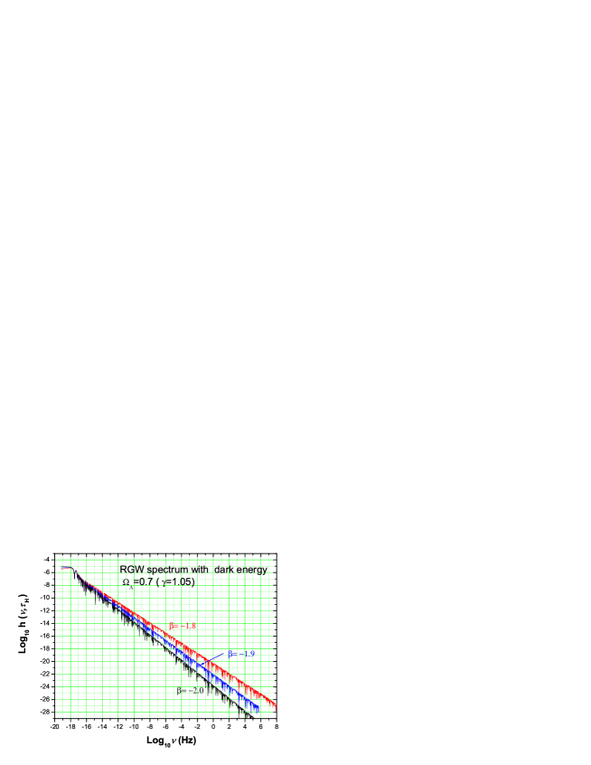
Figure 1: For a fixed $\gamma=1.05$, the exact spectrum $h(\nu,\tau_{H})$ is plotted for three inflationary models of $\beta=-1.8,-1.9,-2.0$, respectively.

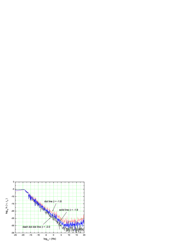
Figure 2: The numerical spectra $h(k,\tau_{H})$ in the accelerating universe for $\beta=-1.8,-1.9$ and $-2.0$, respectively.

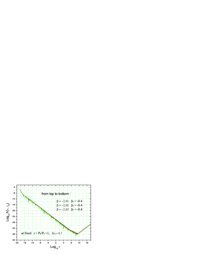
Figure 3: The exact spectra $h(k,\tau_{H})$ in the accelerating universe for $\beta=-2.01,-2.02$ and $-2.03$, respectively.

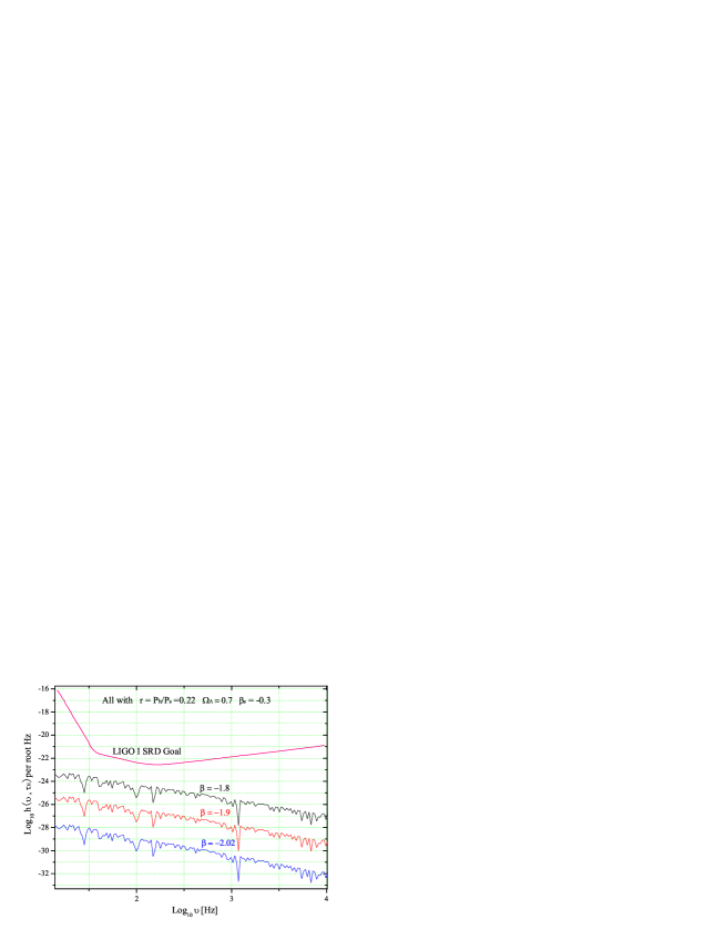
Figure 4: For $\gamma=1.05$ the root mean square spectrum $h(\nu,\tau_{H})/\sqrt{\nu}$ is plotted for the models of $\beta=-1.8,-1.9,-2.02$ to compare with the sensitivity curve from S5 of LIGO.[35]

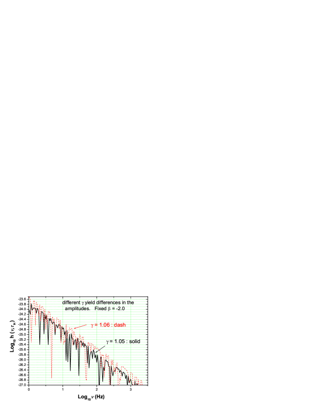
Figure 5: The amplitude of $h(\nu,\tau_{H})$ for the model $\gamma=1.06$ is $\sim 50\%$ higher than that of model $\gamma=1.05$.

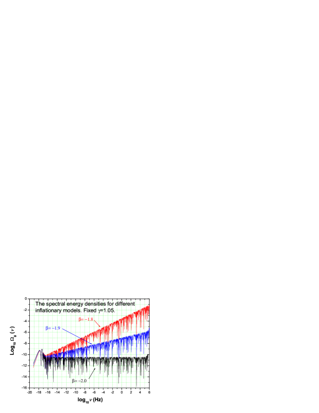
Figure 6: The spectral energy density $\Omega_{g}(\nu)$ is plotted for the models of $\beta=-1.8$, $\beta=-1.9$, and $\beta=-2.0$. The model $\beta=-1.8$ is ruled out by BBN constraint.

Fig. 4 compares the root mean square spectrum $h(\nu,\tau_{H})/\sqrt{\nu}$ of the model $\gamma=1.05$ with the sensitivity of LIGO I SRD [35]^-[37] in the frequency range $\nu=10\sim 10^{4}$Hz.

The spectrum $h(\nu,\tau_{H})$ depends on the dark energy $\Omega_{\Lambda}$ through the parameter $\gamma$. In Fig. 5 we have plotted the spectra in a narrow range of frequencies. It is seen that the amplitude in the model $\gamma=1.06$ is about $\sim 50\%$ greater than that in the model $\gamma=1.05$. That is, in the accelerating Universe with $\Omega_{\Lambda}=0.65$ the amplitude of relic GW is $\sim 50\%$ higher than the one with $\Omega_{\Lambda}=0.7$. This difference is probably difficult to detect at present. However, in principle, it does provide a new way to tell the dark energy fraction $\Omega_{\Lambda}$ in the Universe.

Let us examine the spectral energy density $\Omega_{g}(\nu)$ and its constraints. Fig. 6 is the the plots of $\Omega_{g}(\nu)$ defined in Eq. (14) for $\gamma=1.05$. If we use the result LIGO third science run[36, 37] of the energy density bound for the flat spectrum with $\Omega_{0}<8.4\times 10^{-4}$ in the $69-156$ Hz band, then the model $\beta=-1.8$ is ruled out, but the models $\beta\leq-1.9$ survive. However, this LIGO constraint is not as stringent as the constraint by the so-called nucleosynthesis bound. [38]^-[40]

$$\int\Omega_{g}(\nu)\,d(\log\nu)\leq 0.56\times 10^{-5}.$$ (19)

Note that this is bound on the total GW energy density integrated over all frequencies. The integrand function should also have a bound $\Omega_{g}(\nu)<0.56\times 10^{-5}$ in the interval of frequencies $\delta(\log\nu)\simeq 1$. By this constraint it is also seen from Fig. 6 that only the model $\beta=-2.0$ are still robust.

We have also obtained the following expressions for the analytic approximate spectrum

$$h(k,\tau_{H})=A\left(\frac{k}{k_{H}}\right)^{2+\beta},\,\,\,\,\,k\leq k_{E};$$ (20)

$$h(k,\tau_{H})\approx A\left(\frac{k}{k_{H}}\right)^{\beta-1}\frac{1}{(1+z_{E})^{3+\epsilon}},\,\,\,\,\,k_{E}\leq k\leq k_{H};$$ (21)

$$h(k,\tau_{H})\approx A\left(\frac{k}{k_{H}}\right)^{\beta}\frac{1}{(1+z_{E})^{3+\epsilon}},\,\,\,\,\,k_{H}\leq k\leq k_{2};$$ (22)

$$h(k,\tau_{H})\approx A\left(\frac{k}{k_{H}}\right)^{\beta+1}\frac{k_{H}}{k_{2}}\frac{1}{(1+z_{E})^{3+\epsilon}},\,\,\,\,\,\,\,k_{2}\leq k\leq k_{s};$$ (23)

$$h(k,\tau_{H})\approx A\left(\frac{k_{s}}{k_{H}}\right)^{\beta_{s}}\frac{k_{H}}{k_{2}}\left(\frac{k}{k_{H}}\right)^{\beta-\beta_{s}+1}\frac{1}{(1+z_{E})^{3+\epsilon}},\,\,\,\,\,\,\,k_{s}\leq k\leq k_{1},$$ (24)

where the small parameter $\epsilon\equiv(1+\beta)(1-\gamma)/\gamma$. Approximately $\frac{1}{(1+z_{E})^{3+\epsilon}}\sim\frac{1}{(1+z_{E})^{3}}=\Omega_{m}/\Omega_{\Lambda}$. This extra factor reflects the effects of acceleration caused by the dark energy. Some of other works on RGW can be found in Refs.[41]$-$[45], and the effects of neutrino free-streaming have been recently computed in Ref.[46]$-$[49].

3 CMB Polarization

At the beginning, I mentioned that the magnetic polarization of CMB gives another way to detect RGW. During the era prior to the decoupling in the early Universe, the Thompson scattering of anisotropic radiation by free electrons can give rise to the linear polarization only, so we only consider the polarized distribution function of photons $f=(I_{l},I_{r},U)$ whose components are associated with the Stokes parameters: $I=I_{l}+I_{r}$ and $Q=I_{l}-I_{r}$. The evolution of the photon distribution function is given by the Boltzmann equation[50]

$$\frac{\partial f}{\partial\tau}+\hat{n}^{i}\frac{\partial f}{\partial x^{i}}=-\frac{d\nu}{d\tau}\frac{\partial f}{\partial\nu}-q(f-J),$$ (25)

where $\hat{n}^{i}$ is the unit vector in the direction $(\theta,\phi)$ of photon propagation, $q$ is the differential optical depth and has the meaning of scattering rate. The scattering term $q(f-J)$ describes the effect of the Thompson scattering by free electrons, and the term $-\frac{d\nu}{d\tau}\frac{\partial f}{\partial\nu}$ reflects the effect of variation of frequency due to the metric perturbations through the Sachs-Wolfe formula

$$\frac{1}{\nu}\frac{d\nu}{d\tau}=\frac{1}{2}\frac{\partial h_{ij}}{\partial\tau}\hat{n}^{i}\hat{n}^{j}.$$ (26)

In the presence of perturbations $h_{ij}$, either scalar or tensorial, the distribution function will be perturbed and can be written as

$$f(\theta,\phi)=f_{0}\left[\left(\begin{array}[]{c}1\\ 1\\ 0\\ \end{array}\right)+f_{1}\right],$$ (27)

where $f_{1}$ represents the perturbed portion, $f_{0}(\nu)$ is the usual blackbody distribution. The tensorial type perturbations $h_{ij}$, representing the RGW, has two independent, $+$ and $\times$, polarization.

$$h_{ij}=h^{+}_{ij}+h^{\times}_{ij}=h^{+}\epsilon^{+}_{ij}+h^{\times}\epsilon^{\times}_{ij}.$$

To simplify the Boltzmann equation (25), for the $h_{ij}=h^{+}\epsilon^{+}_{ij}$ polarization, one writes $f_{1}$ in the form[8, 13]

$$f_{1}=\frac{\zeta}{2}\left(1-\mu^{2}\right)\cos 2\phi\left(\begin{array}[]{c}1\\ 1\\ 0\end{array}\right)+\frac{\beta}{2}\left(\begin{array}[]{c}(1+\mu^{2})\cos 2\phi\\ -(1+\mu^{2})\cos 2\phi\\ 4\mu\sin 2\phi\end{array}\right),$$ (28)

where $\zeta\propto I_{l}+I_{r}=I$ represents the anisotropies of photon distribution, and $\beta\propto I_{l}-I_{r}=Q$ represents the polarization of photons. From the Boltzmann equation, upon taking Fourier transformation, retaining only the terms linear in $h_{ij}$, and performing the integration over $d\mu$, one arrives at a set of two equations for the $+$ polarization, [13, 18, 51]

$$\dot{\xi}_{k}+\left[ik\mu+q\right]\xi_{k}=\frac{d\ln f_{0}}{d\ln\nu_{0}}\dot{h}^{+}_{k},$$ (29)

$$\dot{\beta}_{k}+\left[ik\mu+q\right]\beta_{k}=\frac{3q}{16}\int^{1}_{-1}d\mu^{\prime}\left[\left(1+\mu^{\prime 2}\right)^{2}\beta_{k}-\frac{1}{2}\left(1-\mu^{\prime 2}\right)^{2}\xi_{k}\right].$$ (30)

where $\xi_{k}\equiv\zeta_{k}+\beta_{k}$, the over dot $``\cdot"$ denotes $d/d\tau$. For the blackbody spectrum $f(\nu_{0})$ in the Rayleigh-Jeans zone one has $\frac{d\ln f_{0}(\nu_{0})}{d\ln\nu_{0}}\approx 1$. The equations are the same for the $\times$ polarization. In the following we simply omit the sub-index $k$ of wavenumber, the GW polarization notation, $+$ or $\times$, since both $h^{+}$ and $h^{\times}$ are similar in computations. In general, it is difficult to give the exact solution of $\beta$ and $\xi$, but once derived, they can be expanded in terms of the Legendre functions

$$\xi(\mu)=\sum_{l}(2l+1)\xi_{l}P_{l}(\mu),~{}~{}~{}\,\,\beta(\mu)=\sum_{l}(2l+1)\beta_{l}P_{l}(\mu),$$

with the Legendre components

$$\xi_{l}(\tau)=\frac{1}{2}\int_{-1}^{1}\,d\mu\,\xi(\tau,\mu)P_{l}(\mu),~{}~{}~{}\,\,\beta_{l}(\tau)=\frac{1}{2}\int_{-1}^{1}\,d\mu\,\beta(\tau,\mu)P_{l}(\mu).$$ (31)

It can be shown that the spectrum for electric type polarization is given by

$$C_{l}^{\rm GG}=\frac{1}{16\pi}\int\,\left|\frac{(l+2)(l+1)\beta_{l-2}}{(2l-1)(2l+1)}+\frac{6(l-1)(l+2)\beta_{l}}{(2l+3)(2l-1)}+\frac{l(l-1)\beta_{l+2}}{(2l+3)(2l+1)}\right|^{2}\,k^{2}dk,$$ (32)

the spectrum for magnetic type polarization is given by

$$C_{l}^{\rm CC}=\frac{1}{4\pi}\int\,\left|\frac{(l+2)\beta_{l-1}}{2l+1}+\frac{(l-1)\beta_{l+1}}{2l+1}\right|^{2}\,k^{2}dk.$$ (33)

As Eq. (29) shows, one needs the time derivative of $\dot{h}(\tau)$ to solve for $\xi$ and $\beta$. For both polarization, $+,\times$, the wave equation of the relic GW has been given in Eq. (12). The initial condition is taken to be

$$h(\tau=0)=h(k),~{}~{}\dot{h}(\tau=0)=0,$$ (34)

with the primordial power spectrum

$$\frac{k^{3}}{2\pi^{2}}|h(k)|^{2}=P_{h}(k)=A_{T}\left(\frac{k}{k_{0}}\right)^{n_{T}},$$ (35)

where $A_{T}$ is the amplitude, $k_{0}=0.05$ Mpc^-1 is the pivot wavenumber, and $n_{T}$ is the the tensor spectrum index. Inflationary models generically predicts $n_{T}\approx 0$, a nearly scale-invariant spectrum. The resulting $\dot{h}(\tau_{d})$ is plotted in Fig. 7.

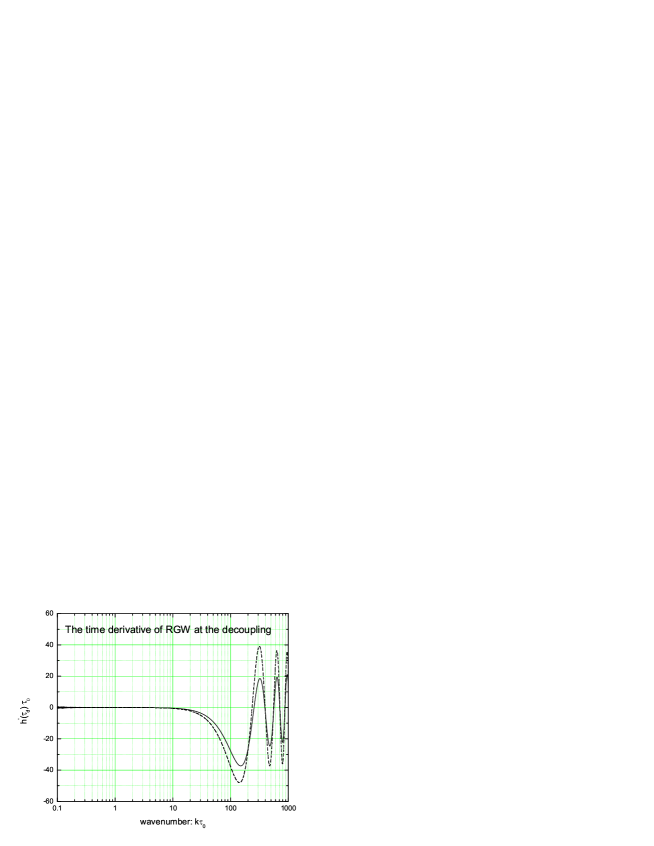
Figure 7: The derivative of RGWs $\dot{h}(\eta_{d})$ as a function of $k$. The solid line is the sudden transition approximation, the dash line is that of the WKB approximation, which is nearly overlapped with the dot line of the numerical result.

One solves the ionization equations during the recombination to give the differential optical depth $q$. Then one obtains the visibility function $V(\tau)$,

$$V(\tau)=q(\tau)e^{-\kappa(\tau_{0},\tau)},$$ (36)

which satisfies $\int_{0}^{\tau_{0}}V(\tau)d\tau=1$ and describes the probability that a given photon last scattered at time $\tau$, where the optical depth function $\kappa(\tau_{0},\tau)$ is related to $q(\tau)$ by $q(\tau)=-d\kappa(\tau_{0},\tau)/d\tau$. [52]^-[54] Fig. 8 shows the profile of $V(\tau)$ by the the numerical result from the CMBFAST, which is sharply peaked around the last scattering. In calculation it is usually fitted by a Gaussian form[16][55]

$$V(\tau)=V(\tau_{d})\exp\left(-\frac{(\tau-\tau_{d})^{2}}{2\Delta\tau_{d}^{2}}\right),$$ (37)

where $\tau_{d}$ is the the decoupling time, and $\Delta\tau_{d}$ is the thickness of decoupling. The WMAP data[33] gives $\Delta\tau_{d}/\tau_{0}=0.00143$. Then, taking $V(\tau_{d})\tau_{0}=279$ in (37) yields a fitting shown in Fig. 8, which has large errors, compared with the numerical one. To improve the fitting of $V(\tau)$, we take the following analytic expressions, consisting of two half-Gaussian functions,[56]

$$V(\tau)=V(\tau_{d})\exp\left(-\frac{(\tau-\tau_{d})^{2}}{2\Delta\tau_{d1}^{2}}\right),~{}~{}~{}(\tau<\tau_{d});$$ (38)

$$V(\tau)=V(\tau_{d})\exp\left(-\frac{(\tau-\tau_{d})^{2}}{2\Delta\tau_{d2}^{2}}\right),~{}~{}~{}(\tau>\tau_{d});$$ (39)

with $\Delta\tau_{d1}/\tau_{0}=0.00110$, $\Delta\tau_{d2}/\tau_{0}=0.00176$, and $(\Delta\tau_{d1}+\Delta\tau_{d2})/2=\Delta\tau_{d}$. Fig. 8 shows that the half-Gaussian model fits the numerical one much better than the Gaussian fitting. This difference will subsequently cause a variation in the polarization spectra.

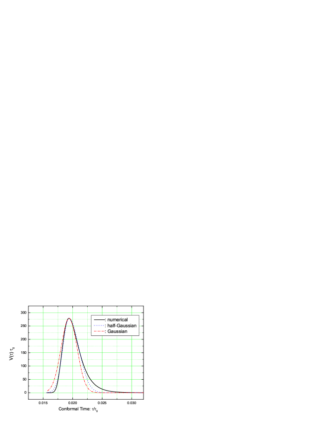
Figure 8: The visibility function $V(\tau)$ around the decoupling. The half-Gaussian model improves the Gaussian model by $\sim 11.5\%$.

We now look for an approximate and analytic solution of Eqs. (29) and (30). On smaller scales the photon diffusion will cause some damping in the anisotropy and polarization. Taking care of this effect to the second order of the small parameter $1/q\ll 1$, by some analysis one arrives at the expression for the component of the polarization

$$\beta_{l}(\tau_{0})=\frac{1}{10}\Delta\tau_{d}\,i^{l}\int_{0}^{\tau_{0}}d\tau V(\tau)\dot{h}(\tau)j_{l}(k(\tau-\tau_{0}))\int_{1}^{\infty}\frac{dx}{x}e^{-\frac{3}{10}\kappa(\tau)x}e^{-\frac{7}{10}\kappa(\tau)},$$ (40)

where $\kappa(\tau)\equiv\kappa(\tau_{0},\tau)$, $x\equiv\kappa(\tau^{\prime})/\kappa(\tau)$, and $d\tau^{\prime}=\frac{dx}{x}\Delta\tau_{d}$ as an approximation. The integration $\int d\tau$ involving $V(\tau)$, which has a factor of the form $e^{-a(\tau-\tau_{d})^{2}}$. As a stochastic quantity, $\dot{h}(\tau)$ contains generally a mixture of oscillating modes, such as $e^{ik\tau}$ and $e^{-ik\tau}$, and so does the spherical Bessel function $j_{l}(k(\tau-\tau_{0}))$. Thus $\dot{h}(\tau)j_{l}(k(\tau-\tau_{0}))$ generally contains terms $\propto e^{-ibk(\tau-\tau_{0})}$, where $b\in[-2,2]$. Using the formula

$$\int_{-\infty}^{\infty}e^{-ay^{2}}e^{ibky}dy=e^{-\frac{(bk)^{2}}{4a}}\int_{-\infty}^{\infty}e^{-ay^{2}}dy,$$

and $V(\tau)$ in Eq. (38) and (39), the integration is approximated by

$$\int_{0}^{\tau_{0}}d\tau V(\tau)\dot{h}(\tau)j_{l}(k(\tau-\tau_{0}))\approx\frac{1}{2}D(k)\dot{h}(\tau_{d})j_{l}(k(\tau_{d}-\tau_{0}))\int_{0}^{\tau_{0}}d\tau V(\tau).$$ (41)

where

$$D(k)\equiv\frac{1}{2}[e^{-\alpha(k\Delta\tau_{d1})^{2}}+e^{-\alpha(k\Delta\tau_{d2})^{2}}],$$ (42)

and $\alpha$ takes values in the range $[0,2]$, depending on the phase of $\dot{h}(\tau)j_{l}(k(\tau-\tau_{0}))$. Here we take $\alpha$ as a parameter. For the Gaussian visibility function one would have $D(k)\equiv e^{-\alpha(k\Delta\tau_{d})^{2}}$. The remaining integrations in $\beta_{l}$ is

$$\int_{0}^{\tau_{0}}d\tau V(\tau)\int_{1}^{\infty}\frac{dx}{x}e^{-\frac{3}{10}\kappa(\tau)x}e^{\frac{-7}{10}\kappa(\tau)}=\int_{0}^{\infty}d\kappa e^{-\frac{17}{10}\kappa}\int_{1}^{\infty}\frac{dx}{x}e^{-\frac{3}{10}\kappa x}=\frac{10}{17}\ln\frac{20}{3}.$$ (43)

This number is the outcome from the second order of the tight-coupling limit, differing the first order result $\frac{10}{7}\ln\frac{10}{3}$ in Ref. [55]. Finally one obtains

$$\beta_{l}(\tau_{0})=\frac{1}{17}\ln\frac{20}{3}i^{l}\Delta\tau_{d}\dot{h}(\tau_{d})j_{l}(k(\tau_{d}-\tau_{0}))D(k),$$ (44)

which contains explicitly the time derivative $\dot{h}(\tau_{d})$ of RGW. Substituting this back into Eqs. (32) and (33) yields the polarization spectra

$$C^{XX}_{l}=\frac{1}{16\pi}\left(\frac{1}{17}\ln\frac{20}{3}\right)^{2}\int P_{Xl}^{2}(k(\tau_{d}-\tau_{0}))|\dot{h}(\tau_{d})|^{2}\Delta\tau_{d}^{2}D^{2}(k)\,k^{2}dk,$$ (45)

where “X” denotes “G” or “C” the type of the CMB polarization. For the electric type

$$P_{Gl}(x)=\frac{(l+2)(l+1)}{(2l-1)(2l+1)}j_{l-2}(x)-\frac{6(l-1)(l+2)}{(2l-1)(2l+3)}j_{l}(x)+\frac{l(l-1)}{(2l+3)(2l+1)}j_{l+2}(x),$$ (46)

and for the magnetic type

$$P_{Cl}(x)=\frac{2(l+2)}{2l+1}j_{l-1}(x)-\frac{2(l-1)}{2l+1}j_{l+1}(x).$$ (47)

To completely determine $C^{XX}_{l}$ above, we need the initial amplitude $\dot{h}(\tau_{d})$ to be fixed through Eq. (35) by the initial spectrum $P_{h}(k)=rP_{s}$, associated to the scalar spectrum $P_{s}$ by Eq. (16). WMAP observation[57] gives the scalar spectrum

$$P_{s}(k_{0})=2.95\times 10^{-9}A(k_{0}),$$ (48)

with $k_{0}=0.05$ Mpc^-1 and $A(k_{0})=0.8$. Taking the scale-invariant spectrum with $n_{T}=0$ in (35), then the amplitude $A_{T}$ in (35) depends on $r$.

The polarization spectrum $C_{l}^{CC}$ of magnetic type, calculated from our analytic formulae (45) and from the numerical CMBFAST,[58] are shown in Fig. 9. The approximate analytic result is quite close to that of the numerical CMBFAST for the first three peaks that are observable.

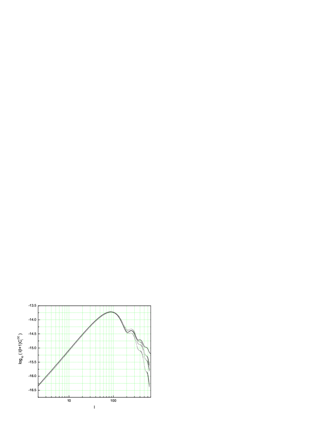
Figure 9: The magnetic polarization spectrum $C^{CC}_{l}$ with the ratio $r=1$. The solid line is the numerical result from the CMBFAST. The upper dot line is the result from the half-Gaussian visibility function with $\alpha=1.7$, the middle dot line is with $\alpha=2$, and the lower dot line is the Gaussian fitting with $\alpha=2$. The half-Gaussian fitting is better than the Gaussian one.

The location of the peaks:

In (46) and (47) the spherical Bessel function $j_{l}(k(\tau_{d}-\tau_{0}))$ is peaked at $l\simeq k(\tau_{0}-\tau_{d})\simeq k\tau_{0}$ for $l\gg 1$. So the peak location of the power spectra are directly determined by

$$C_{l}^{XX}\propto\left|\dot{h}(\tau_{d})\right|^{2}k^{2}D^{2}(k)\left.\right|_{k=l/\tau_{0}}.$$ (49)

The factor $D(k)$ has a larger damping at larger $l$, so the first peak of the power spectrum has the highest amplitude. From our analytic solution one has $\dot{h}(\tau_{d})^{2}\propto[j_{2}(k\tau_{d})]^{2}$, which peaks at $k\tau_{d}\simeq 3$. Thus $C_{l}^{XX}$ peaks around

$$l\simeq k\tau_{0}\simeq 3\tau_{0}/\tau_{d}.$$ (50)

A lower dark energy component leads to smaller $\tau_{0}/\tau_{d}$. For $\Omega_{\Lambda}=0.65$, $0.73$ and $0.80$, respectively, and with fixed $\Omega_{b}=0.044$, $\Omega_{dm}=1-\Omega_{\Lambda}-\Omega_{b}$, a numerical calculation yields that $\tau_{0}/\tau_{d}\simeq 50.1$, $51.3$ and $53.6$, respectively. A smaller $\Omega_{\Lambda}$ will also shift the peaks $\dot{h}(\tau_{d})$ slightly to larger scales. Together, a smaller $\Omega_{\Lambda}$ will shift the peak of $C_{l}^{XX}$ to larger scales, as demonstrated in Fig. 10. This suggests a new way to study the cosmic dark energy. The baryon component also influence the peak location. A higher baryon density $\Omega_{b}$ makes the peak to large scales, as is demonstrated in Fig. 11.

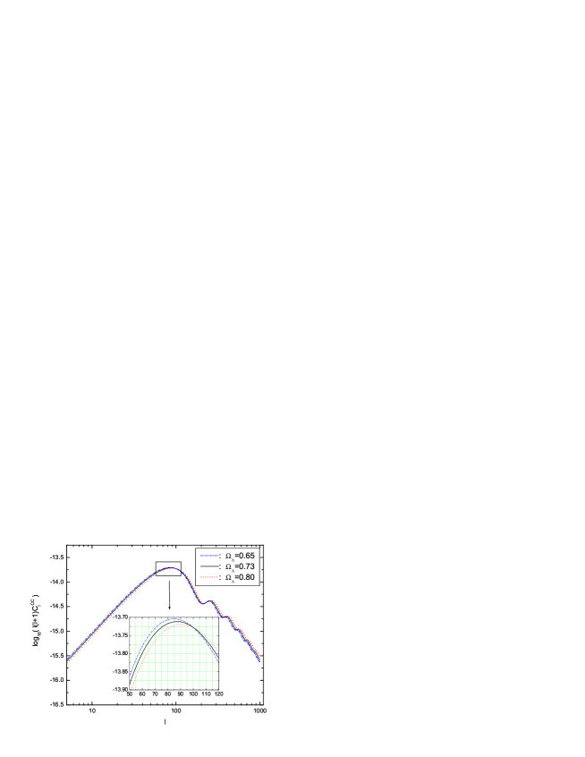
Figure 10: $C_{l}^{CC}$ depends weakly on the dark energy. A smaller $\Omega_{\Lambda}$ yields a higher amplitude and shifts the peaks to larger scales.

The height of amplitude:

$C_{l}^{XX}$ depend on the decoupling thickness $\Delta\tau_{d}$ and the damping factor $D(k)$: $C_{l}^{XX}\propto\Delta\tau_{d}^{2}D(k)^{2}$. For a fixed $k$, the smaller $\Delta\tau_{d}$ leads to a larger $D(k)$. $\Delta\tau_{d}$ is mainly determined by the baryon density $\Omega_{b}$ of the Universe. A higher $\Omega_{b}$ corresponds to a smaller $\Delta\tau_{d}$. The total effect is that a higher $\Omega_{b}$ leads to a lower $C_{l}^{CC}$, as is shown in Fig. 11. Besides, a smaller $\Omega_{\Lambda}$ yields a higher amplitude, as seen in Fig. 10.

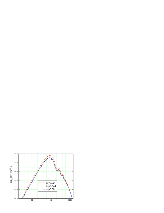
Figure 11: The dependence of $C_{l}^{CC}$ on $\Omega_{b}$ in the $\Lambda$CDM universe with $\Omega_{\Lambda}=0.73$, $\Omega_{dm}=1-\Omega_{\Lambda}-\Omega_{b}$, and $r=1$. A larger $\Omega_{b}$ yields a lower amplitude and shifts the peaks slightly to larger scales.

The influence of the inflation on $C_{l}^{XX}$:

The inflation models determine the ratio $r$ and the amplitude $|\dot{h}(\tau_{d})|$ in (35), including the spectrum index $n_{T}$ of RGW. A larger $r$ yields a larger $|\dot{h}(\tau_{d})|$ and a higher polarization. A larger $n_{T}$ yields higher polarization spectra.

The more recent treatments can be found in Refs. [56], [59] $-$ [62].

4 Conclusion and Discussion

Our calculations of RGW have shown that in the low frequency range the peak of spectrum is now located at a frequency $\nu_{E}\simeq(\frac{\Omega_{m}}{\Omega_{\Lambda}})^{1/3}\nu_{H}$, where $\nu_{H}$ is the Hubble frequency, and there appears a new segment of spectrum between $\nu_{E}$ and $\nu_{H}$. In all other intervals of frequencies $\geq\nu_{H}$, the spectral amplitude acquires an extra factor $\frac{\Omega_{m}}{\Omega_{\Lambda}}$, due to the current acceleration, otherwise the shape of spectrum is similar to that in the decelerating models. The amplitude for the model $\Omega_{\Lambda}=0.65$ is $\sim 50\%$ greater than that of the model $\Omega_{\Lambda}=0.7$. The spectrum sensitively depends on the inflationary models, and a larger $\beta$ yields a flatter spectrum, producing more power. Both the LIGO bound and the nucleosynthesis bound point out that the inflationary model $\beta=-1.8$ is ruled out, but the model $\beta=-2.0$ is still alive.

Our analytic polarization spectra of CMB has the following improvements.

(i) The analytic result of CMB polarization is quite close to the numerical result from the CMBFAST code. The dependence of polarization on the dark energy and the baryons are analyzed. A smaller $\Omega_{\Lambda}$ yields a higher amplitude and shifts the peaks to large scales. A larger $\Omega_{b}$ yields a lower amplitude and shifts the peaks to large scales.

(ii) Our half-Gaussian approximation of the visibility function fits analytically better than the simple Gaussian fitting, and its time integration yields a parameter-dependent damping factor. This improves the spectrum $\sim 30\%$ around the second and third peaks.

(iii) The second order of tight coupling limit reduces the amplitude of spectra by $\sim 58\%$, comparing with the first order.

(iv) A larger value of the spectrum index $n_{T}$ of RGW and a larger ratio $r$ yield higher polarization spectra.

ACKNOWLEDGMENT: Y. Zhang would like to thank the organizers of Third International ASTROD Symposium on Laser Astrodynamics, Space Test of Relativity and Gravitational-Wave Astronomy. He also thanks Dr. L. Q. Wen for interesting discussions. The work has been supported by the CNSF No. 10773009, SRFDP, and CAS. W. Zhao has been supported by Graduate Student Research Funding from USTC.

References

- [1] V. A. Rubakov, M.V. Sazhin and A.V. Veryaskin, Phys. Lett. B 115 (1982) 189.
- [2] R. Fabbri and M. D. Pollock, Phys. Lett. B 125 (1983) 445.
- [3] L. Abbott and M. Wise, Nuc. Phys. B 237 (1984) 226.
- [4] L. F. Abbott and D. D. Harari, Nucl. Phys. B 264 (1986) 487.
- [5] B. Allen, Phys. Rev. D 37 (1988) 2078.
- [6] V. Sahni, Phys. Rev. D 42 (1990) 453.
- [7] L. P. Grishchuk, Ann. NY Acad. Sci. 302 (1977) 439.
- [8] M. M. Basko and A. G. Polnarev, Mon. Not. R. Astron. Soc. 191 (1980) 207.
- [9] N. Kaiser, Mon. Not. R. Astron. Soc. 202 (1983) 1169;
- [10] J.R. Bond and G. Efstathiou, Astrophys. J. Lett. 285 (1984) L45;
- [11] J.R. Bond and G. Efstathiou, Mon. Not. R. Astron. Soc. 226 (1987) 655.
- [12] M. M. Basko and A. G. Polnarev, Mon. Not. R. Astron. Soc. 191 (1980) 207.
- [13] A. Polnarev, Sov. Astron. 29 (1985) 6.
- [14] R. A. Frewin, A.G. Polnarev and P. Coles, Mon. Not. R. Astron. Soc. 266 (1994) L21.
- [15] B. Keating et al, Astrophys. J. 495 (1998) 580.
- [16] D. Harari and M. Zaldarriaga, Phys. Lett. B 310 (1993) 96.
- [17] M. Zaldarriaga and D. D. Harari, Phys. Rev. D 52 (1995) 3276.
- [18] K. L. Ng and K. W. Ng, Astrophys. J. 445 (1995) 521.
- [19] A. Kosowsky, Ann. Phys. 246 (1996) 49.
- [20] M. Kamionkowski, A. Kosowsky and A. Stebbins, Phys. Rev. D 55 (1997) 7368.
- [21] R. Crittenden, R. L. Davis and P. J. Steinhardt, Astrophys. J. 417 (1993) L13.
- [22] D. Coulson, R. Crittenden and N. Turok, Phys. Rev. Lett. 73 (1994) 2390.
- [23] R. Crittenden, D. Coulson, and N. Turok, Phys. Rev. D 52 (1995) 5402.
- [24] U. Seljak and M. Zaldarriaga, Phys. Rev. Lett. 28 (1997) 2054.
- [25] W. Hu and M. White, Phys. Rev. D 56 (1997) 597.
- [26] W. T. Ni, Chin. Phys. Lett. 22 (2005) 33.
- [27] W. T. Ni, Int. J. Mod. Phys. D 14 (2005) 901.
- [28] L. Grishchuk, Class. Quant. Grav. 14 (1997) 1445.
- [29] L. Grishchuk, Lecture Notes Physics 562, (2001) 164.
- [30] Y. Zhang et al, Class. Quant. Grav. 22 (2005) 1383 .
- [31] Y. Zhang and W. Zhao, Chin. Phys. Lett. 22 (2005) 1817.
- [32] Y. Zhang et al, Class. Quant. Grav. 23 (2006) 3783.
- [33] D. N. Spergel et al, Astrophys. J. Suppl. 148 (2003) 175.
- [34] D. N. Spergel et al, Astrophys. J. Suppl. 170 (2007) 377.
- [35] http://www.ligo.caltech.edu/advLIGO.
- [36] B. Abbott et al, Phys. Rev. Lett. 94, (2005) 181103.
- [37] B. Abbott et al, Phys. Rev. Lett. 95 (2005) 221101.
- [38] M. Maggiore, Phys. Rep. 331 (2000) 283.
- [39] M. R. G. Maia, Phys. Rev. D 48 (1993) 647.
- [40] M. R. G. Maia and J.D. Barrow, Phys. Rev. D 50 (1994) 6262.
- [41] H. Tashiro, K. Chiba and M. Sasaki, Class. Quant. Grav. 21 (2004) 1761.
- [42] A. B. Henriques, Class. Quant. Grav. 21 (2004) 3057.
- [43] G. Gong, Class. Quant. Grav. 21 (2004) 5555.
- [44] W. Zhao and Y. Zhang, Phys. Rev. D 74 (2006) 043503.
- [45] S. Wang, Y. Zhang, T. Y. Xia and H. X. Miao, accepted, Phys. Rev. D 77 (2008) 104016.
- [46] S. Weinberg, Phys. Rev. D 69 (2004) 023503.
- [47] D. A. Dicus and W. W. Repko, Phys. Rev. D 72 (2005) 088302.
- [48] Y. Watanabe and E. Komatsu, Phys. Rev. D 73 (2006) 123515.
- [49] H. X. Miao and Y. Zhang, Phys. Rev. D 75 (2007) 104009.
- [50] S. Chandrasekhar, Radiative Transfer, Dover, New York (1960).
- [51] Y. Zhang, H. Hao and W. Zhao, ChA&A 29 (2005) 250.
- [52] P. J. E. Peebles, Astrophys. J. 153 (1968) 1.
- [53] B. Jones and R. Wyse, Astron. Astrophys. 149 (1985) 144.
- [54] W. Hu and N. Sugiyama, Astrophys. J. 444 (1995) 489.
- [55] J. R. Pritchard and M. Kamionkowski, Ann. Phys. 318 (2005) 2.
- [56] W. Zhao and Y. Zhang, Phys. Rev. D 74 (2006) 083006.
- [57] H. V. Peiris et al, Astrophys. J. Suppl. 148 (2003) 213.
- [58] U. Seljak and M. Zaldarriaga, Astrophys. J. 469 (1996) 437.
- [59] D. Baskaran, L. Grishchuk and A. Polnarev, Mon. Not. R. Astron. Soc. 370 (2006) 799.
- [60] B. Keating, A. Polnarev, N. Miller and D. Baskaran, Int. J. Mod. Phys. B 21 (2006) 2459.
- [61] A. Polnarev, N. Miller and B. Keating, arXiv:0710.3649 astro-ph.
- [62] L. P. Grishchuk, arXiv:0707.3319 astro-ph.