Strain-Induced Conduction Band Spin Splitting in GaAs from First Principles Calculations
Athanasios N. Chantis
Theoretical Division, Los Alamos National Laboratory,
Los Alamos, New Mexico, 87545, USA
Manuel Cardona
Max Planck Institut für Festkörperforschung, Heisenbergstrasse 1, D-70569 Stuttgart, Germany
Niels E. Christensen
Department of Physics and Astronomy, University of Aarhus, DK-8000 Aarhus C, Denmark
Darryl L. Smith
Theoretical Division, Los Alamos National Laboratory,
Los Alamos, New Mexico, 87545, USA
Mark van Schilfgaarde
School of Materials, Arizona State University,
Tempe, Arizona, 85287-6006, USA
Takao Kotani
School of Materials, Arizona State University,
Tempe, Arizona, 85287-6006, USA
Axel Svane
Department of Physics and Astronomy, University of Aarhus, DK-8000 Aarhus C, Denmark
Robert C. Albers
Theoretical Division, Los Alamos National Laboratory,
Los Alamos, New Mexico, 87545, USA
Abstract
We use a recently developed self-consistent approximation to present
first principles calculations of the conduction band spin
splitting in GaAs under strain.
The spin orbit
interaction is taken into account as a perturbation to the scalar
relativistic hamiltonian. These are the first calculations of conduction
band spin splitting under deformation based on a quasiparticle approach; and because the
self-consistent scheme accurately reproduces the relevant band
parameters, it is expected to be a reliable predictor of spin splittings.
We also discuss the spin relaxation time under strain and show that
it exhibits an in-plane anisotropy, which can be exploited to obtain the magnitude and sign
of the conduction band spin splitting experimentally.
The increasing prospect of utilizing spin electronics with conventional semiconductors,
calls for quantitative predictions of the spin relaxation of electrons
in these materials. Awschalom and Flatté (2007); Kato et al. (2003)
In semiconductors without inversion symmetry, the spin relaxation rate is related to the relativistic splitting in
the conduction band, an effect which also induces spin precession and is relevant for spin
transport and injection. Riechert et al. (1984); Alvarado et al. (1985); Alvarado and Renaud (1992); Misra et al. (2005)
In zinc-blende semiconductors, which are the most promising for spintronic applications, it is
widely accepted that D’yakonov-Perel’ (DP) D’yakonov and Perel’ (1971) is the dominant spin relaxation mechanism.
Generally speaking, this mechanism is present when the spin degeneracy of the conduction band is lifted.
The spin splitting can be viewed as a k-dependent effective magnetic
field which under certain
scattering conditions relaxes the average spin of the ensemble.
The strength of the effective field depends on the material.
In the general form we can add this field to
the Hamiltonian as an effective Zeeman term, ,
where (with the dimensions of energy) is proportional to .
In the zinc-blende crystal structure there is no inversion symmetry; this leads
to an field with components Dresselhaus (1955); Rashba and Sheka (1961)
(1)
where , the indices obey a cyclic relationship (), and is a
constant that depends on the bulk properties of the material. This effective field was first introduced
by Dresselhaus Dresselhaus (1955).
In uniaxially deformed crystals there is an additional effective field D’yakonov et al. (1986); Pikus et al. (1988); Bir and Pikus (1962); Safarov and Titkov (1983)
(2)
is the strain tensor, and are material-dependent constants.
The first part of the effective field originates from off-diagonal components of the strain tensor
while the second part originates from diagonal ones. The second part appears only due to
the spin orbit mixing of and states and therefore should be much
weaker than the first part Cardona et al. (1984), but a numerical estimation of has not yet been performed, probably because of uncertainties concerning the states.
The data for the values of , and in various zinc-blende
semiconductors are very sparse. The most studied case is GaAs. However, the
experimental data for show a wide range of values, between 11.0 and 34.5 eVÅ3. myn
Theoretical calculations of this parameter also show a wide range of predicted values.
Calculations based on kp method predict a value between 25 and 30 eVÅ3. myn
However, a first principles calculation by Cardona et al Cardona et al. (1988) predicted a value of
15 eVÅ3. Our recent first principles calculation Chantis et al. (2006) predicted
a value of 8.5 eVÅ3,
a lot smaller than the commonly cited value of 27.5 eVÅ3. Recently, Krich et al Krich and Halperin (2007)
used a semi-classical approach to estimate the effect of on
the mean and variance of the conductance in closed quantum dots and compared the results of their
model with the experiment in Ref. Zumbuhl et al., 2005. They were able to reach
a good agreement only when they used our value of , suggesting that the value of
in GaAs must be around 9 eVÅ3.
Also our current knowledge of and in GaAs is far from being satisfactory.
The magnitude of was estimated experimentally in Refs. Beck et al., 2006 and Gorelenok et al., 1986
to be 8.12.5 eVÅ and 3.9 eVÅ, respectively. The values of
calculated with Linear Combination of Atomic Orbitals (LCAO) and pseudopotentials are 3.75
and 11.24 eVÅ, respectively Cardona et al. (1988).
The calculations are able to define also the sign of ;
in Ref. Cardona et al., 1988 it was found to be opposite to that of . ccf
No other attempt has been made since to calculate the sign of .
To our knowledge the magnitude and sign of
has not been estimated experimentally nor theoretically so far. Although,
M. I. D’yakonov et al D’yakonov et al. (1986) showed that the spin
relaxation time has a very weak dependence on applied pressure
upon application of [100] strain, possibly indicating that the magnitude of
is negligibly small.
In this work we use a recently developed ab inito method
based on the approximation to predict
these parameters for GaAs.
We will try to answer the important questions about the strengths and
signs of the spin splittings caused by the two mechanisms, Eqs. 1 and 2.
II Method
The approximation can
be viewed as the first term in the expansion
of the non-local energy dependent self-energy
in the screened Coulomb interaction . From a more physical point of view
it can be interpreted as a dynamically screened Hartree-Fock approximation plus
a Coulomb hole contribution Hedin and Lundqvist (1969).
It is also a prescription for mapping the non-interacting Green function to the dressed
one, . In the Quasiparticle Self-consistent (QS) method a prescription is given on how to map
to a new non-interacting Green function .
This is used for the input to a new iteration; we repeat the procedure
until converegence is reached.
Thus QS is a self-consistent perturbation theory, where the
self-consistency condition is constructed to minimize the size of the
perturbation. QS is parameter-free, independent of basis set and of
the LDA Kotani et al. (2007).
The method is described in great detail in Refs. Kotani et al., 2007 and van Schilfgaarde
et al., 2006a.
It has been shown that QS reliably describes the band structure in a wide
range of materials van Schilfgaarde
et al. (2006b); Faleev et al. (2004); Chantis et al. (2006, 2007).
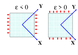
Figure 1: The left panel represents the applied deformation for
and the right for .
The QS method in the current implementation uses the
Full Potential Linear Muffin Tin Orbital (FP-LMTO)
method Andersen (1975); Methfessel et al. (2000),
so we make no approximations for the shape of the crystal potential.
The smoothed LMTO basis includes orbitals
with and both 3 and 4 are included
in the basis. are added in the form of local orbitals van Schilfgaarde
et al. (2006a)–an orbital
strictly confined to the augmentation sphere, which has no envelope function at all.
As QS gives the self-consistent
solution at the scalar relativistic level,
we add the spin-orbit operator, ,
as a perturbation (it is not included in the self-consistency cycle).
It has also been shown that the QS method systematically overestimates the fundamental
band gap in semiconductors by an amount of a few tenths of an eV, independent of the
magnitude of the gap van Schilfgaarde
et al. (2006b).
This error is related to the fact that the
vertex correction is not taken into account in the method and when taken into account
a nearly perfect agreement with experiment is achieved Shishkin et al. (2007).
Here, in order to obtain highly accurate results with less computational effort,
we take a simple but somewhat heuristic approach to correct the error.
We considered a ‘hybridized’ QS+LDA Hamiltonian with
(3)
In Ref. Chantis et al., 2006 we found
that for all III-V and II-VI semiconductors studied a value of gives
excellent agreement of calculated band gap and other important band parameters with
experiment.
Table 1: Important band parameters for GaAs. and are the energies of the
first two conduction bands at the -point. and are the spin-orbit splittings between
and for valence and conduction bands, respectively.
is the conduction band effective mass at
. Energies are in eV; is in eV, and
are in eV. An asterisk in front of the value indicates that this is a calculated value from
another theoretical method.
3.9555From Table IX of Ref. Cardona et al., 1988; where only the absolute value is reported, 4.0666From Ref. Cardona et al., 1984; where only the absolute value is reported,
5.3333From Ref. Gorelenok et al., 1986; Pikus et al., 1988; where only the absolute value is reported, 8.12.5444From Ref. Beck et al., 2006; where only the absolute value is reported,
*-3.74777Calculated with Pseudopotentials; From Table IX of Ref. Cardona et al., 1988,*-11.2888Calculated with LCAO; From Table IX of Ref. Cardona et al., 1988,*2.0999Calculated with Pseudopotentials; From Ref. Cardona et al., 1984,
*5.0101010Calculated with LCAO; From Ref. Cardona et al., 1984,*4.9111111Calculated with the three-band kp method; From Ref. Pikus et al., 1988
+2.13
+1.7
All band parameters presented in Table I, except and , are calculated
for the undistorted lattice structure. All signs are presented with the convention
that the anion is at the origin and cation at (0.25,0.25,0.25).
We see that overall the QS is in good agreement with experiment but the
‘hybridized’ QS+LDA Hamiltonian is in even better agreement.
For and we calculate self-consistently the self-energy
and charge density under the corresponding deformation. We found that
if instead we use the self-consistent self energy of the undistorted structure
the value of differs from that presented in Table I by 5.
In these calculations
the atomic positions were allowed to relax within LDA in order to account for the
displacement of the anion and cation sublattices relative to each other.
For a pure shear deformation in the [111] direction this displacement can be
viewed as a length change of the [111] bond described by the internal
strain parameter , .
Our calculated value of is 0.53, in good agreement with previous calculations
Rönnow et al. (1999); Blacha et al. (1984)
We apply two different deformations, the first of which is described by the following strain tensor:
(4)
where 0.0025186, -0.0049628
and 0.0074814.
This tensor conserves the volume and
induces the related term in .
To separate this term from the related term we also
performed a calculation with a deformation described by the following strain tensor:
(5)
This strain tensor conserves the volume only to first order of deformation
but only the first term ( related) is present in .
III results
III.1 Spin splittings
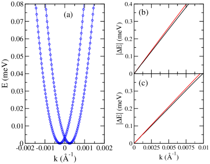
Figure 2:
(a) The shift of the conduction band minimum away from the point in GaAs under deformation
given by Eq. 4 (’hybridized’ method). (b) The magnitude of the conduction
band splitting along the [010] direction for the case of the ’hybridized’ Hamiltonian, red line with
deformation (4) black line with deformation (5) (c) same as (b) but
for QS Hamiltonian.
In Fig. 2
we show the -dependence of the conduction band splitting along [010]
for the case of ’hybridized’ and QS calculations.
Figure 2(a) shows the energy dispersion around the point for the
case of the ’hybridized’ Hamiltonian and the deformation given by Eq. 4.
Along the [010] direction vanishes and the dispersion is given
by
(6)
where
(7)
and the strain components were introduced in Sect. II.
Correspondingly, the conduction band minimum shifts to
(8)
In Figs. 2(b) and (c) we show the magnitude of the splitting along
the [010] direction for the case of ’hybridized’ and QS Hamiltonians, respectively.
The black solid lines are for strain (4) and the red solid lines
for (5). The slope of the red line is equal to
(9)
while the slope of the black line is equal to
(10)
Hence
(11)
and
(12)
The magnitudes of and extracted with this procedure are given in Table I.
As expected, in the case of the ’hybridized’ method they are slightly larger than
in the QS because the ’hybridized’ band structure has a smaller band gap.
However, the ratio of remains nearly constant; it is equal to 3.197 in the ’hybridized’
method and 3.171 in QS. The magnitude of is in good agreement
with experiments in both the QS and the ’hybridized’ methods but the latter should be
trusted more due to better agreement of the other band parameters with experimental values.
We also note that in the experimental determination of , the terms were considered to be negligible.
This corresponds to extracting the value of directly from ; according to
our calculations this would yield an inaccurate value of eV with an error of 5, much
less than the experimental error in Ref. Beck et al. (2006).
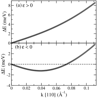
Figure 3:
(a) The conduction band splitting along the [110] direction for the case of ’hybridized’
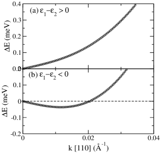
Hamiltonian, applied strain (5) for (c) same as (a) but for . Figure 4:
(a) The conduction band splitting along the [110] direction for the case of ’hybridized’ Hamiltonian,
under deformation (14) with (b) same as
(a) but for .
The is highly anisotropic and completely vanishes in certain directions but
is present for a general direction. It is therefore interesting to compare
with . We start by comparing to .
When we apply deformation (5), the dispersion along the [110]
direction is
(13)
Thus the Dresselhaus and the stress terms can either add or subtract, depending
on the relative sign of and .
If they subtract the splitting will be zero at
i.e. the spin splitting reverses its sign at .
In Table I it is seen that , which means that for
the deformation (5) the spin splitting along [110] will change sign
at Å-1.
As shown in Fig. 1,
can be either negative or positive,
therefore such cancellation will always occur depending on the sign of the product.
For example, if , whether it occurs for or depends on the sign of .
In Ref. Chantis et al., 2006 we determined the sign of according to
conventions in Ref. Cardona et al., 1988. Here we will determine the sign of relative
to the sign of by simply plotting along [110] for
positive and negative . In Fig. 3 we show such plot for
the deformation (5) with positive and negative .
The splitting is linear only in the vicinity of the point,
away from the point the cubic term is clearly visible. For the
two contributions add (Fig. 3(a)) but for they oppose
each other (Fig. 3(b)); for the cubic term
dominates and the splitting becomes positive. It is clear that and
have the same sign
(according to the convention used here they are both positive).
The sign of B is defined in a similar way. We apply the deformation:
(14)
So that . Then the splitting along the [110] direction is
.
if crosses zero for then and have
opposite signs, otherwise and have the same sign.
As can be seen in Fig. 4 we find that .
III.2 Spin relaxation
After having reliably determined the values of material parameters that
dictate the spin relaxation rate in GaAs it will be interesting to estimate
the spin relaxation time for a deformation like the one given by Eq. 4.
In the Appendix we have derived the average spin relaxation time when
both and are present
(15)
(16)
(17)
Where denotes axis parallel to the vector and
perpendicular to it. Namely, and are the axes along the [10] and
[110] crystal directions, respectively.
We see that there is an in-plane
anisotropy induced by the simultaneous presence of
and strain components (a similar anisotropy was observed for the circular piezo-birefringence and
confinement-induced circular birefringence in GaAs Koopmans et al. (1998)).
We can write the strain tensor (14) in these axes: with
,
and .
If we apply a uniaxial pressure (stress), , along [110] in this system of coordinates, then using the compliance constants , and
we find , and , hence,
and .
According to Eqs. 15 and 16 the difference between
the inverse of the spin relaxation time along [10] and [110] is equal to
(18)
Hence, an experimental
setup similar to the one described above should be able to measure a linear increase of
the difference (18) with the square of applied pressure.
The rate of increase should be proportional
to . In the experiment of Ref. D’yakonov et al., 1986 the authors measured the increase of
the spin relaxation time with applied pressure along [100]. Such strain will only induce the
terms in Eqs. (15)-(17). If we assume that the
applied strain is large enough to ignore the Dresselhaus term, then the spin
relaxation time should be isotropic and should increase linearly with the square of applied strain.
However, unlike the experimental setup proposed here the
rate of increase is proportional to .
The experiment proposed here is independent of Dresselhaus terms no matter how small is the deformation,
also the linear increase is proportional to instead of , hence it may be easier to detect.
Provided that the orientation of the As-Ga bond has been previousely determined, this
experiment can be used to find the sign of relative to that of from the sign of the difference (18).
IV conclusion
We have presented first principles calculations of the magnitude and sign of bulk constants
that govern the DP spin scattering in GaAs under strain. To our knowledge, this was the first
estimation of magnitude and sign of . We find that both and have the
same sign as . Our value of is in good agreement with experiments.
We have derived an expression for the spin relaxation time of electrons under
a strain given by Eq. 4 and showed that the in-plane spin relaxation is anisotropic
in this case. We proposed an experiment that can exploit this anisotropy to deduce
the magnitude and sign of .
Acknowledgements.
The work at Los Alamos was supported by DOE Office of Basic Energy Sciences Work Proposal Number 08SCPE973.
V Appendix: Spin scattering rate
The momentum dependent spin relaxation time tensor is defined as:
(19)
and
(20)
Here and the overbar denotes averaging over all directions of .
is the momentum scattering time for an electron with energy and
(21)
where is the electron scattering cross section and
the Legendre polynomials. Here it is
assumed that the electron scattering is elastic, the electron energy spectrum is
isotropic and the scattering cross section
depends only on the scattering angle .
is the total effective field and in
our case we can write:
(22)
with the components as given in Eqs. (1) and
(2). We apply a strain like that of tensor Eq.
(4) with the constraint
, so as to conserve the volume. Then
(23)
where .
To facilitate the discussion let’s write also explicitly
the components of the Dresselhaus field:
(24)
Then we can write
(25)
The first integral on the RHS is
(26)
The second integral on the RHS is
(27)
The third integral on the RHS is
So we get
(28)
In a similar way we obtain
and
(29)
For the off-diagonal components we get
(30)
The first three integrals on the RHS are equal to zero.
With the form of strain field given by Eq. (23) the
last term can be written as
(31)
All other are equal to zero.
Therefore according to equations (1) and (2)
for the spin relaxation time of an electron with energy E we find
(32)
(33)
(34)
Then the average spin relaxation time is
(35)
(36)
(37)
where and the brackets denote averaging over energies. For example for
the Maxwell distribution
.
By transforming the above tensor to the principal system of coordinates we obtain:
(38)
(39)
(40)
Where denotes axis parallel to the vector and
perpendicular to it. Namely, and are the axes along the [10] and
[110] crystal directions, respectively.
Equations (38) and (39) signal an in-plane
anisotropy induced by the simultaneous presence of
and .
References
Awschalom and Flatté (2007)
D. D. Awschalom
and M. E.
Flatté, Nature Phys
3, 153 (2007).
Kato et al. (2003)
Y. K. Kato,
R. C. Myers,
A. C. Gossard,
and D. D.
Awschalom, Nature
427, 50 (2003).
Riechert et al. (1984)
H. Riechert,
S. F. Alvarado,
A. N. Titkov,
and V. I.
Safarov, Phys. Rev. Lett.
52, 2297 (1984).
Alvarado et al. (1985)
S. F. Alvarado,
H. Riechert, and
N. E. Christensen,
Phys. Rev. Lett. 55,
2716 (1985).
Alvarado and Renaud (1992)
S. F. Alvarado and
P. Renaud,
Phys. Rev. Lett. 68,
1387 (1992).
Misra et al. (2005)
S. Misra,
S. Thulasi, and
S. Satpathy,
Phys. Rev. B 72,
195347 (2005).
D’yakonov and Perel’ (1971)
M. I. D’yakonov
and V. I.
Perel’, Sov. Phys. JETP
33, 1053 (1971).
Dresselhaus (1955)
G. Dresselhaus,
Phys. Rev. 100,
580 (1955).
Rashba and Sheka (1961)
E. I. Rashba and
V. I. Sheka,
Sov. Phys. Solid State 3,
1735 (1961).
D’yakonov et al. (1986)
M. I. D’yakonov,
V. A. Maruschak,
V. I. Perel’,
and A. N.
Titkov, Sov. Phys. JETP
63, 655 (1986).
Pikus et al. (1988)
G. E. Pikus,
V. A. Maruschak,
and A. N.
Titkov, Sov. Phys. Semicond
22, 115 (1988).
Bir and Pikus (1962)
G. L. Bir and
G. E. Pikus,
Sov. Phys. Solid State 3,
2221 (1962).
Safarov and Titkov (1983)
V. I. Safarov and
A. N. Titkov,
Physica 117B&118B,
497 (1983).
Cardona et al. (1984)
M. Cardona,
V. A. Maruschak,
and A. N.
Titkov, Solid State Communications
50, 701 (1984).
(15)
See auxiliary material (EPAPS) in Phys. Rev. Lett. 98, 226802
(2007).
Cardona et al. (1988)
M. Cardona,
N. E. Christensen,
and G. Fasol,
Phys Rev B 38,
1806 (1988).
Chantis et al. (2006)
A. N. Chantis,
M. van Schilfgaarde,
and T. Kotani,
Phys. Rev. Lett. 96,
086405 (2006).
Krich and Halperin (2007)
J. J. Krich and
B. I. Halperin,
Phys. Rev. Lett. 98,
226802 (2007).
Zumbuhl et al. (2005)
D. M. Zumbuhl,
J. B. Miller,
C. M. Marcus,
D. Goldhaber-Gordon,
J. J. S. Harris,
K. Campman, and
A. C. Gossard,
Phys. Rev. B 72,
081305 (2005).
Beck et al. (2006)
M. Beck,
C. Metzner,
S. Malzer, and
G. H. Dohler,
Europhysics Lett. 75,
597 (2006).
Gorelenok et al. (1986)
A. T. Gorelenok,
B. A. Marushchak,
and A. N.
Titkov, Akad. Nauk SSSR, Ser. Fiz.
50, 290 (1986).
(22)
In Eq. (6.3) of Ref. Cardona et al., 1988 a kp
perturbation expression for C (labelled V2) is given. It involves the product
of three matrix elements, of momentum, strain and spin-orbit coupling. They
must be evaluated using wavefunctions with consistent phases for the choice
of atomic positions. An inconsistency in these functions led to the wrong
(negative) sign of C which should actually be positive, in agreement with
that found in the present calculations.
Hedin and Lundqvist (1969)
L. Hedin and
S. Lundqvist, in
Solid State Physics, edited by
H. Ehrenreich,
F. Seitz, and
D. Turnbull
(Academic, New York, 1969),
vol. 23, p. 1.
Kotani et al. (2007)
T. Kotani,
M. van Schilfgaarde,
and S. V.
Faleev, Phys. Rev. B
76, 165106
(2007).
van Schilfgaarde
et al. (2006a)
M. van Schilfgaarde,
T. Kotani, and
S. V. Faleev,
Phys. Rev. B 74,
245125 (2006a).
van Schilfgaarde
et al. (2006b)
M. van Schilfgaarde,
T. Kotani, and
S. Faleev,
Phys. Rev. Lett. 96,
226402 (2006b).
Faleev et al. (2004)
S. V. Faleev,
M. van Schilfgaarde,
and T. Kotani,
Phys. Rev. Lett. 93,
126406 (2004).
Chantis et al. (2007)
A. N. Chantis,
M. van Schilfgaarde,
and T. Kotani,
Phys. Rev. B 76,
165126 (2007).
Andersen (1975)
O. K. Andersen,
Phys. Rev. B 12,
3060 (1975).
Methfessel et al. (2000)
M. Methfessel,
M. van Schilfgaarde,
and R. A.
Casali, Lecture Notes in Physics, vol.
535 (Springer-Verlag, Berlin, 2000,
2000).
Shishkin et al. (2007)
M. Shishkin,
M. Marsman, and
G. Kresse,
Phys Rev Lett 99,
246403 (2007).
Madelung (1996)
O. Madelung,
Semiconductors Basic Data
(Springer-Verlag, Berlin, 1996).
Rönnow et al. (1999)
D. Rönnow,
N. E. Christensen,
and M. Cardona,
Phys. Rev. B 59,
5575 (1999).
Blacha et al. (1984)
A. Blacha,
H. Presting, and
M. Cardona,
phys. stat. sol. 126,
11 (1984).
Koopmans et al. (1998)
B. Koopmans,
P. V. Santos,
and M. Cardona,
phys. stat. sol. (b) 205,
419 (1998).