Excitations of the One Dimensional Bose-Einstein Condensates in a Random Potential

Abstract

We examine bosons hopping on a one-dimensional lattice in the presence of a random potential at zero temperature. Bogoliubov excitations of the Bose-Einstein condensate formed under such conditions are localized, with the localization length diverging at low frequency as $\ell(\omega)\sim 1/\omega^{\alpha}$. We show that the well known result $\alpha=2$ applies only for sufficiently weak random potential. As the random potential is increased beyond a certain strength, $\alpha$ starts decreasing. At a critical strength of the potential, when the system of bosons is at the transition from a superfluid to an insulator, $\alpha=1$. This result is relevant for understanding the behavior of the atomic Bose-Einstein condensates in the presence of random potential, and of the disordered Josephson junction arrays.

One of the most challenging problems of quantum many body physics is the behavior of stongly interacting matter in a disordered environment. In this paper we investigate the universal properties of superfluids in such systems, near the superfluid insulator transition. Interest in this problem arises in many independent contexts, in work on granular superconducting films and wires Haviland et al. (1989); Frydman et al. (2002); Lau et al. (2001), Helium condensates in vycor Crowell et al. (1997), and recent experiments on Bose condensates in optical traps. In particular, issues such as the expansion of a noninteracting Bose condensate through a random potential Sanchez-Palencia et al. (2007), excitations in an interacting Bose Einstein condensate in a random potential Bilas and Pavloff (2006); Lugan et al. (2007), and the possibility of the observation of the Bose glass phase Fallani et al. (2007); Lye et al. (2007) were explored in very recent theoretical and experimental papers. As important is the possibility of investigating the behavior of disordered superconductors in a controlled fashion using Josephson junction arrays, as in Refs. Chow et al. (1998); Castellanos-Beltran and Lehnert (1997); Rimberg et al. (1997). In low dimensional quantum systems, where symmetry broken phases are very fragile, we expect the most dramatic manifestations of the interplay of disorder and interactions. The existence of the Bose-glass phase was established in Refs. Giamarchi and Schultz (1988); Fisher et al. (1989), where the scaling and renormalization group (RG) picture of the 1d superfluid-insulator transition at weak disorder was also established. Recently, much theoretical progress was afforded through real-space RG approaches in the case of dissipative Hoyos et al. (2007) and closed Altman et al. (2004, 2008) bosonic chains, where the properties of the SF-insulator transition at strong disorder were established.

In this paper, we study the excitations of the superfluid phase in a bosonic chain with a strongly random potential and interactions, near the SF-insulator transition. Capitalizing on the real-space RG understanding of this transition Altman et al. (2004, 2008), we analyze the localization length of phonons (i.e., Bogoliubov quasiparticles) as a function of their frequency and wave number. Deep in the superfluid phase, when the random potential is weak, the phonon localization length $\ell(\omega)$ at small $\omega$ diverges as Ishii (1973); Ziman (1982); Bilas and Pavloff (2006)

$$\ell(\omega) \sim 1/{\omega^{\alpha}},$$ (1)

$$\alpha = 2.$$ (2)

This result, in particular, formed the basis of the analysis in Refs. Bilas and Pavloff (2006); Lugan et al. (2007). Using the renormalization group analysis of Ref. Altman et al. (2004) and the study of random elastic chains of Ref. Ziman (1982), we show that Eq. (2) does not apply everywhere in the superfluid regime. In a finite region of parameter space on the superfluid side near the superfluid-insulator transition, Eq. (2) fails, and is replaced by the law

$$\alpha=g,$$ (3)

where $1\leq g\leq 2$. The meaning of the parameter $g$ will be elucidated later in the paper. Furthermore, as the system approaches the transition to the insulating regime, $g$ decreases. Exactly at the transition $g=1$, and Eq. (1) acquires a correction to scaling:

$$\ell(\omega)\sim\left({\ln^{2}\omega}\right)/{\omega}.$$ (4)

Eqs. (3) and (4) constitute the main result of our paper.

Our analysis begins by considering a one-dimensional disordered Bose-Hubbard model with many particles per site. Its Hamiltonian is

$$H=\sum_{k}\left[\frac{U_{k}}{2}\left(-i\frac{\partial}{\partial\phi_{k}}+n_{k}\right)^{2}-J_{k}\cos\left(\phi_{k+1}-\phi_{k}\right)\right].$$ (5)

This Hamiltonian describes a chain of sites, connected to their nearest neighbors by a Josephson hopping with a random strength, $J_{k}$. $U_{k}$ is the strength of the onsite repulsion, and $n_{k}\in\left[-\frac{1}{2},\frac{1}{2}\right]$ are random offset charges. The hopping, charging and offsets are randomly distributed with probability densities $P_{J}(J)$, $P_{U}(U)$, and $P_{n}(n)$.

In the strong-disorder limit a real space renormalization group analysis can be employed to gradually eliminate sites with anomalously large $J_{k}$ or or local charging gap, $\Delta_{k}=U_{k}(1-2|n_{k}|)$ Altman et al. (2004, 2008). The remaining sites are described by the same Hamiltonian but with the renormalized probability distributions. The system of Eq. (5) then emerges as either a superfluid or an insulator; the latter could be either a Mott insulator, a Mott glass, Bose glass, or random-singlet glass, depending on the strength, relative and absolute, of various types of disorder present. If the bosonic system is a superfluid, the distribution of $J$ renormalizes towards the universal limiting function

$$P_{J}(J)=CJ^{g-1}.$$ (6)

with $C$ providing normalization. The superfluid is described by $g\geq 1$ with its value decreasing as the critical point at $g=1$ is approached; in particular, as disorder increases, g decreases. At the same time,

$$P_{U}(U)\sim\frac{1}{U^{2}}\exp\left(-\frac{\Omega f}{U}\right),$$ (7)

where $f$ flows to $0$ along the renormalization group trajectories and $\Omega$ is the decreasing UV cutoff scale of the renormalized Hamiltonian, i.e., its largest hopping or gap. We now proceed to show that the same parameter $g$ appearing in the distribution (6) controls the localization length of low-frequency phonons, as expressed in Eq. (3).

At the final stages of the renormalization, as long as $g\geq 1$, the system is a superfluid and the possibility that the phase difference at adjacent sites slips through $2\pi$ can be safely ignored. Moreover, since the Hamiltonian is no longer periodic in $\phi_{k}$ it is now possible to do a gauge transformation to eliminate $n_{k}$ in Eq. (5), marking the ability of the superfluid to screen arbitrary offset charges. Then one may expand the cosine, to find the effective Hamiltonian (up to an unimportant additive overall constant)

$$H=\sum_{k}\left[-\frac{U_{k}}{2}\frac{\partial^{2}}{\partial\phi_{k}^{2}}+\frac{J_{k}}{2}\left(\phi_{k+1}-\phi_{k}\right)^{2}\right].$$ (8)

The Hamiltonian Eq. (8) is quadratic, and thus we obtain full information by analyzing it at the classical level. Its classical equations of motion are

$$\omega^{2}U_{k}^{-1}\phi_{k}=J_{k}\left(\phi_{k}-\phi_{k+1}\right)+J_{k-1}\left(\phi_{k}-\phi_{k-1}\right),$$ (9)

where $\omega$ is the angular frequency. These describe phonons in a chain of random masses connected by random springs. The masses are $m_{k}\sim 1/U_{k}$, while the spring constants are proportional to $J_{k}$. Ref. Ziman (1982) presented the solution to this problem (referred to as “Dyson type II”) for the case when $P_{U}(U)=\delta(U-U_{0})$ (that is, nonrandom uniform charging energies $U_{k}=U_{0}$) and $P_{J}(J)=CJ^{g-1}$ with $J\in[0,J_{0}]$. It was found that the average density of states is constant at low frequency,

$$\rho(\omega)=\left\langle\,\sum_{n}\delta\left(\omega-\omega_{n}\right)\,\right\rangle\sim\ {\rm const}.$$ (10)

Here $\omega_{n}$ are the frequencies of the phonons described by (9) and brackets denote averaging over random $J_{k}$. A constant density of states at low frequency is of course a feature shared with non-random elastic chains. The phonons which are the solutions of Eq. (9), however, are all localized. Their localization length obeys Eq. (1) (at small $\omega$) with

$$\begin{array}[]{cc}\alpha=2,\,g\geq 2;&\alpha=g,\,1\leq g\leq 2.\end{array}$$ (11)

These results are compatible with our claim in beginning of this paper, Eqs. (3) and (4). Nevertheless, the uniform-$U$ treatment leading to Eqs. (11) cannot be considered a derivation of the localization length results in our problem: the random boson problem has charging energies $U_{k}$ which are also randomly distributed. Below we show that the results given in Eqs. (10) and (11) are valid even if $U_{k}$ are random, as long as the probability of observing anomalously small $U_{k}$ is not too large. In addition we show that the uniform-$U$ results for $g=1$ exhibit strong corrections to scaling [see Eq. (31)].

Let us first confirm that the fully random Bosonic chain, Eq. (8), also has a finite constant density of states at low frequencies, as in (10). Consider the classical ground state of a system of $N+1$ sites described by Eq. (9), where the first grain’s phase $\phi_{0}$ is kept fixed at $\phi_{0}=0$, and a force $h$ is applied conjugate to the phase $\phi_{N}$ of the last grain. The equilibrium values of the variables $\phi_{k}$ can be found by minimizing the energy

$$E=\frac{1}{2}\sum_{k=0}^{N-1}J_{k}\left(\phi_{k}-\phi_{k+1}\right)^{2}-h\,\phi_{N}.$$ (12)

which yields:

$$\phi_{k}=h\sum_{l=0}^{k-1}J^{-1}_{l},\,0<k\leq N.$$ (13)

Alternatively, $\phi_{k}$ can be computed in the following way. Introducing the variables $\psi_{k}=\phi_{k}/\sqrt{U_{k}}$, we can find $\psi_{N}$ by inverting the matrix ${\cal H}_{kl}$ defined by the expression

$$\frac{1}{2}\sum_{k=0}^{N-1}J_{k}\left(\psi_{k}\sqrt{U_{k}}-\psi_{k+1}\sqrt{U_{k+1}}\right)^{2}\equiv\frac{1}{2}\sum_{k,l=1}^{N}{\cal H}_{kl}\psi_{k}\psi_{l}.$$ (14)

Then

$$\phi_{k}=\sqrt{U_{k}U_{N}}\,G_{kN}~{}h.$$ (15)

where $G$ is a matrix inverse to ${\cal H}$. In particular, we are interested in $k=N$ case when Eq. (15) can be rewritten as

$$\phi_{N}=h\sum_{n}\frac{{C_{n}\left[\phi_{N}^{(n)}\right]}^{2}}{\omega_{n}^{2}},\ C_{n}=\left[{\sum_{k=1}^{N}\frac{\left(\phi^{(n)}_{k}\right)^{2}}{U_{k}}}\right]^{-1}.$$ (16)

Here $\phi_{k}^{(n)}$ are the normalized solutions to the eigenmode equation Eq. (9) with the boundary conditions $\phi_{0}=0$ at the beginning of the chain, and with the frequency $\omega_{n}$, labelled by the index $n$.

Next we compare the two expressions for $\phi_{k}$ at $k=N$, Eq. (13) and Eq. (16). We observe that for the probability distribution $P(J)=J^{g-1}$, as long as $g>1$,

$$\left<\phi_{N}\right>=h\left<{\sum_{k=0}^{N-1}J_{k}^{-1}}\right>\sim N.$$ (17)

On other other hand,

$$\phi_{N}=N\int d\omega\,\rho(\omega)\,\frac{{C_{\omega}\left[\phi_{N}^{(\omega)}\right]}^{2}}{\omega^{2}},$$ (18)

where $\phi^{(\omega)}$ refers to the eigenmode at frequency $\omega$, and $\rho(\omega)$ is the density of states. Clearly, unless the density of states is strongly suppressed at small $\omega$, the integral (18) diverges due to small $\omega$ contributions. At small $\omega$, the localization length exceeds the system size, thus $\phi_{N}^{(\omega)}\sim 1/\sqrt{N}$. At the same time, $\left<1/U_{k}\right>$ is finite, which means that $C_{\omega}$ is both $\omega$ and $N$ independent. Suppose $\rho(\omega)\sim\omega^{\gamma}$, where $\gamma<1$. Then

$$\phi_{N}\sim\int d\omega\,\frac{\rho(\omega)}{\omega^{2}}\sim\frac{\rho(\omega_{0})}{\omega_{0}},$$ (19)

where $\omega_{0}$ is the smallest frequency of the system, which can be found by

$$\int_{0}^{\omega_{0}}d\omega\,\rho(\omega)\sim\frac{1}{N},\ \omega_{0}\sim\frac{1}{N^{\frac{1}{1+\gamma}}}.$$ (20)

This in turn gives

$$\phi_{N}\sim N^{\frac{1-\gamma}{1+\gamma}}.$$ (21)

Comparison with (17) reveals that $\gamma=0$, i.e., Eq. (10).

We now return to the localization length. First, consider the case of weak random $J_{k}=J_{0}+\delta J_{k}$ and $U_{k}=U_{0}+\delta U_{k}$. Treating $\delta J_{k}$ as a perturbation, it is easy to find the localization length following Refs. John et al. (1982); Gurarie and Chalker (2003). Indeed, the mean free time can be found by the Fermi golden rule, to go as $\tau^{-1}\sim\omega^{2}$, while the mean free path goes as $\sqrt{J_{0}U_{0}}\tau$. The localization length is proportional to the scattering length in 1D, thus $\ell(\omega)\sim\omega^{-2}$.

This calculation however ignores the possibility of the wave scattering off the anomalously small $J_{k}$ or $U_{k}$. Indeed, suppose we have a “weak link” in Eq. (9) where $J_{\rm weak\ link}=j$ on that link is much smaller than $J$ on other links, $j\ll J$. It is straightforward to check that the phonons with wave vector $q\gg j/J$ get reflected off this weak link, while those with wave vector $q\ll j/J$ pass straight through. This is easiest to see if we solve Eq. (9) with the assumptions that all $J_{k}$ are equal to $J_{0}$, while that of the weak link is $j\ll J_{0}$ and all the $U_{k}$ are equal to $U_{0}$. Then the transmission coefficient through the weak link is given by

$$T=\frac{1}{1+q^{2}\frac{J_{0}^{2}}{4j^{2}}},$$ (22)

where $q$ is the dimensionless wave vector which is assumed to be small, or $|q|\ll\pi$. $T$ tends to $1$ at small $q$, and to $0$ at large $q\gg j/J$.

It thus follows that a phonon with wave vector $q$ cannot have a localization length bigger than the average distance between the “weak links” with the strength of their couplings no bigger than $q$ divided by the density of states. Using Eq. (6) we can estimate the average separation between such weak links. We find

$$\int_{0}^{j}dJ~{}J^{g-1}\sim\frac{1}{\ell},$$ (23)

where $\ell$ is the average distance between the weak links $j$. This gives $\ell\sim 1/j^{g}$. Since $j\sim q$, and $q\sim\omega$ due to Eq. (10), the localization length is bounded from above by $\ell\sim 1/\omega^{g}$, thus we arrive at our result, Eq. (3).

Scattering off the small $U_{k}$ can also reflect the short wavelength waves. Taking all $U_{k}$ equal to $U_{0}$, while the “heavy link” (recall that the “masses” are inversely proportional to $U_{k}$) $U_{k}$ equal to $u\ll U_{0}$, and taking all the $J_{k}=J_{0}$ gives the transmission coefficient

$$T=\frac{1}{1+\frac{U_{0}^{2}}{4u^{2}}q^{2}},$$ (24)

equivalent to (22). This, however, does not lead to any corrections to Eq. (3). Indeed, using the same arguments as preceeding Eq. (23), we find

$$\int_{0}^{u}\frac{dU}{U^{2}}\exp\left(-\frac{\Omega f}{U}\right)\sim\exp\left(-\frac{\Omega f}{u}\right)\sim\frac{1}{\ell}.$$ (25)

Here $\ell$ is the typical distance between these “heavy” links. Again taking $u\sim q\sim\omega$, we find

$$\ell\sim\exp\left(\frac{\Omega f}{\omega}\right).$$ (26)

This estimate is much bigger than Eq. (3) and thus the real localization length Eq. (3) remains unaffected. This concludes the derivation of Eqs. (10) and Eqs. (2,3,4).

The analysis of $\ell(\omega)$ above assumed that we probe the phonon modes of the superfluid in the very end of the renormalization group flow, once the power law that controls the distribution $P_{J}(J)\sim J^{g-1}$, has already attained its fixed-line value. While this is valid in the limit of $\omega\rightarrow 0$, corrections to scaling may arise near the critical point. Refs. Altman et al. (2004, 2008) allows us to consider the corrections to this analysis arising from the flow to the SF fixed line. The RG flow for the generic-disorder case is given by:

$$\frac{df}{d\Gamma}=f(1-g),\ \frac{dg}{d\Gamma}=-\frac{1}{2}fg,$$ (27)

where $\Gamma$ is the logartihmic RG flow parameter. In the region close to the critical point, $f=0,\,g=1$, we can solve these equations approximately to give:

$$\begin{array}[]{cc}g\approx 1+\epsilon+\frac{2\epsilon}{e^{\epsilon\Gamma}-1},&f\approx\epsilon^{2}\frac{4e^{\epsilon\Gamma}}{\left(e^{\epsilon\Gamma}-1\right)^{2}}\end{array}$$ (28)

for disorder realizations that flow to $g=1+\epsilon$ with $\epsilon\ll 1$. Flows that terminate at the critical point, however, are given approximately by:

$$\begin{array}[]{cc}g\approx 1+\frac{2}{\Gamma},&f\approx\frac{4}{\Gamma^{2}}.\end{array}$$ (29)

To find the corrections to scaling in the form of $\ell(\omega)$, we first note that it is given by the bare length-scale of renormalized sites once the RG scale reaches $\Gamma=\ln\frac{\omega_{0}}{\omega}$, with $\omega_{0}$ the bare energy scale of the Bose-Hubbard chain. The RG flow of the effective site and bond length is:

$$\frac{d\ell}{d\Gamma}=\ell(f+g).$$ (30)

At the critical point we expect $\ell(\omega)\sim{1/\omega}$; let us first derive the correction to scaling at the critical point. Integrating Eq. (30) using Eq. (29) gives $\ln\ell=\Gamma+2\ln\Gamma/\Gamma_{0}+{\cal O}(1/\Gamma)$, and thus we find the localization length at criticality having a logarithmic correction:

$$\ell(\omega)\sim\left[\ln^{2}\left(\omega/\omega_{0}\right)\right]/\omega.$$ (31)

Off criticality, we find by the same analysis:

$$\ell(\omega)\sim\left[\left(1-\left(\omega/\omega_{0}\right)^{\epsilon}\right)/\epsilon\right]^{2}/\omega^{1+\epsilon}.$$ (32)

In summary, localization properties at low frequency are determined by the parameter $g$. Its value cannot be calculated directly in closed form from the initial disorder distribution, but we can estimate it by following the RG flow using the techniques of Refs. Altman et al. (2004, 2008). In Fig. 1 we demonstrate how initial distributions evolve into the exponent $\alpha$, which is $g$ at the end of the flow.

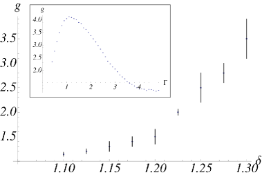
Figure 1: An example of the correspondence between initial distributions, and the exponent $g=\alpha$ at the end of the flow. Main plot: terminal $g$ as a function of the parameter $\delta$ for initial Gaussian coupling distributions $P_{U}(U)\sim e^{-(U-0.3)^{2}/0.7^{2}}$, and $P_{J}(J)\sim e^{-(J-\delta)^{2}/0.4^{2}}$, truncated for $J,U<10^{-4}$. Inset: example of the flow of $g$ vs. the RG flow parameter $\Gamma$ for the Gaussian initial conditions with $\delta=1.125$. The localization exponent $\alpha$ at $\delta=1.25$ is $g$ at the large $\Gamma$ plateau. Each point is averaged over 40 disorder realizations, with the chains of $5\cdot 10^{6}$ sites.

Finally, we remark that the results of this paper should also be valid in the case of the quasi one-dimensional condensates in the presence of random potential (but in the absence of any lattice). Indeed, such condensates are expected to form puddles in the minima of the potential, with nonzero boson hopping amplitudes between the puddles. Then they are expected to mimic (5), and the rest of the analysis of this paper applies.

We acknowledge support from the NSF grant DMR-0449521 and from the NIST - CU seed grant (VG), and from the EPSRC Grant No. EP/D050952/1 (JTC).

References

- Haviland et al. (1989) D. B. Haviland, Y. Liu, and A. M. Goldman, Phys. Rev. Lett. 62, 2180 (1989).
- Frydman et al. (2002) A. Frydman, O. Naaman, and R. C. Dynes, Phys. Rev. B 66, 052509 (2002).
- Lau et al. (2001) C. N. Lau, N. Markovic, M. Bockrath, A. Bezryadin, and M. Tinkham, Phys. Rev. Lett. 87, 217003 (2001).
- Crowell et al. (1997) P. A. Crowell, F. W. Van Keuls, and J. D. Reppy, Phys. Rev. B 55, 12620 (1997).
- Sanchez-Palencia et al. (2007) L. Sanchez-Palencia, D. Clément, P. Lugan, P. Bouyer, G. Shlyapnikov, and A. Aspect, Phys. Rev. Lett. 98, 210401 (2007).
- Bilas and Pavloff (2006) N. Bilas and N. Pavloff, Eur. Phys. J. D. 40, 387 (2006).
- Lugan et al. (2007) P. Lugan, D. Clément, P. Bouyer, A. Aspect, and L. Sanchez-Palencia, Phys. Rev. Lett. 99, 180402 (2007).
- Fallani et al. (2007) L. Fallani, J. E. Lye, V. Guarrera, C. Fort, and M. Inguscio, Phys. Rev. Lett. 98, 130404 (2007).
- Lye et al. (2007) J. E. Lye, L. Fallani, C. Fort, V. Guarrera, M. Mudugno, D. S. Wiersma, and M. Inguscio, Phys. Rev. A 75, 061603 (2007).
- Chow et al. (1998) E. Chow, P. Delsing, and D. B. Haviland, Phys. Rev. Lett. 81, 204 (1998).
- Castellanos-Beltran and Lehnert (1997) M. A. Castellanos-Beltran and K. W. Lehnert (1997), eprint arXiv:0706.2373.
- Rimberg et al. (1997) A. J. Rimberg, T. R. Ho, C. Kurdak, J. Clarke, K. L. Campman, and A. C. Gossard, Phys. Rev. Lett. 78, 2632 (1997).
- Giamarchi and Schultz (1988) T. Giamarchi and H. Schultz, Phys. Rev. B 37, 325 (1988).
- Fisher et al. (1989) M. P. A. Fisher, P. B. Weichman, G. Grinstein, and D. S. Fisher, Phys. Rev. B 40, 546 (1989).
- Hoyos et al. (2007) J. A. Hoyos, C. Kotabage, and T. Vojta, Phys. Rev. Lett. 99, 230601 (2007).
- Altman et al. (2004) Y. Altman, Y. Kafri, A. Polkovnikov, and G. Refael, Phys. Rev. Lett. 93, 150402 (2004).
- Altman et al. (2008) Y. Altman, Y. Kafri, A. Polkovnikov, and G. Refael, Phys. Rev. Lett. 100, 170402 (2008).
- Ishii (1973) K. Ishii, Prog. Theor. Phys. Suppl. 53, 77 (1973).
- Ziman (1982) T. Ziman, Phys. Rev. Lett. 49, 337 (1982).
- John et al. (1982) S. John, H. Sompolinsky, and M. J. Stephen, Phys. Rev. B 27, 5592 (1982).
- Gurarie and Chalker (2003) V. Gurarie and J. T. Chalker, Phys. Rev. B 68, 134207 (2003).