Lifetimes of tidally limited star clusters with different radii

Abstract

We study the escape rate of stars, $\dot{N}$, from clusters with different radii on circular orbits in a tidal field using analytical predictions and direct $N$-body simulations. We find that $\dot{N}$ depends on the ratio $\mbox{$\mathfrak{R}$}\equiv r_{\rm h}/r_{\rm J}$, where $r_{\rm h}$ is the half-mass radius and $r_{\rm J}$ the radius of the zero-velocity surface around the cluster. For $\mbox{$\mathfrak{R}$}\gtrsim 0.05$, the “tidal regime”, there is almost no dependence of $\dot{N}$ on $\mathfrak{R}$. To first order this is because the fraction of escapers per half-mass relaxation time, $t_{\rm rh}$, scales approximately as $\mbox{$\mathfrak{R}$}^{3/2}$, which cancels out the $r_{\rm h}^{3/2}$ term in $t_{\rm rh}$. For $\mbox{$\mathfrak{R}$}\lesssim 0.05$, the “isolated regime”, $\dot{N}$ scales as $\mbox{$\mathfrak{R}$}^{-3/2}$. The dissolution time-scale, $t_{\rm dis}$, falls in three regimes. Clusters that start with their initial $\mathfrak{R}$, $\mathfrak{R}_{i}$, in the tidal regime dissolve completely in this regime and their $t_{\rm dis}$ is, therefore, insensitive to the initial $r_{\rm h}$. Our model predicts that $\mathfrak{R}_{i}$ has to be $10^{-20}-10^{-10}$ for clusters to dissolve completely in the isolated regime. This means that realistic clusters that start with $\mathfrak{R}_{i}\lesssim 0.05$ always expand to the tidal regime before final dissolution. Their $t_{\rm dis}$ has a shallower dependence on $\mathfrak{R}_{i}$ than what would be expected when $t_{\rm dis}$ is a constant times $t_{\rm rh}$. For realistic values of $\mathfrak{R}_{i}$, the lifetime varies by less than a factor of 1.5 due to changes in $\mathfrak{R}_{i}$. This implies that the “survival” or “vital” diagram for globular clusters should allow for more small clusters to survive. We note that with our result it is impossible to explain the universal peaked mass function of globular cluster systems by dynamical evolution from a power-law initial mass function, since the peak will be at lower masses in the outer parts of galaxies. Our results finally show that in the tidal regime $t_{\rm dis}$ scales as $N^{0.65}/\omega$, with $\omega$ the angular frequency of the cluster in the host galaxy.

1 Introduction

Stars escape from clusters due to internal two and three body encounters in which stars get accelerated to velocities higher than the escape velocity. The resulting dissolution time-scale, $t_{\rm dis}$, depends on the number of stars, $N$, and the escape rate, $\dot{N}$, as $\mbox{$t_{\rm dis}$}\equiv-N/\dot{N}$. For a constant $\dot{N}$ the instantaneous value of $t_{\rm dis}$ is the remaining time to total dissolution. For clusters in isolation $t_{\rm dis}$ scales linearly with the half-mass relaxation time, $t_{\rm rh}$ (Ambartsumian, 1938; Spitzer, 1940). The presence of a tidal field speeds up $\dot{N}$ by roughly an order of magnitude (Hénon, 1961; Spitzer & Chevalier, 1973; Giersz & Heggie, 1997). When treating the tidal field as a radial cut-off, as is often done in Fokker Planck and $N$-body simulations (Chernoff & Weinberg, 1990; Gnedin & Ostriker, 1997; Takahashi & Portegies Zwart, 2000) $t_{\rm dis}$ also scales with $t_{\rm rh}$ (Baumgardt 2001, hereafter B01).

Fukushige & Heggie (2000) demonstrated that for a realistic tidal field it is important to consider the finite time it takes stars to escape through one of the Lagrange points. B01 showed that then $\mbox{$t_{\rm dis}$}\propto t_{\rm rh}^{3/4}$. This scaling was also found for more realistic $N$-body simulations that include a stellar mass function and stellar evolution (Vesperini & Heggie 1997; Baumgardt & Makino 2003, hereafter BM03). BM03 only considered the dependence of $t_{\rm rh}$ on cluster mass, $M$, since in their runs the initial half-mass radius, $r_{\rm h}$, and the initial tidal radius are linked, so $r_{\rm h}\propto M^{1/3}$.

Observations of young (extra-galactic) clusters show that the scaling of $r_{\rm h}$ with cluster mass, $M$, and galactocentric distance, $R_{\rm G}$, is considerably shallower: $r_{\rm h}\propto M^{0.1}\,R^{\,0.1}_{\rm G}$ (Zepf et al., 1999; Larsen, 2004; Scheepmaker et al., 2007) than the Roche-lobe filling relation ($r_{\rm h}\propto M^{1/3}\,R_{\rm G}^{\,2/3}$), implying that massive clusters and clusters at large $R_{\rm G}$ are initially under-filling their Roche-lobe.

The relation between $t_{\rm dis}$ and the median cluster radius, $\bar{r}$, was modelled by Wielen (1971) for clusters up to $N=250$. He found that $t_{\rm dis}$ (in Myrs) scales with $\bar{r}^{3/2}$ for $\bar{r}\lesssim 0.01\,r_{\rm J}$, with $r_{\rm J}$ the Jabobi radius, being the radius of the zero-velocity surface around the cluster imposed by the tidal field. This is because for these clusters $\mbox{$t_{\rm dis}$}\propto t_{\rm rh}$. For $\bar{r}\gtrsim 0.05\,r_{\rm J}$ this scaling is not followed any more and $t_{\rm dis}$ is shorter. Large clusters are even more vulnerable to disruption when the effect of passing molecular clouds is included (King, 1958; Wielen, 1985; Gieles et al., 2006).

Tanikawa & Fukushige (2005) modelled the evolution of clusters of larger $N$ that are initially Roche-lobe under-filling using collisionless $N$-body simulations. They confirm that for Roche-lobe filling clusters $\mbox{$t_{\rm dis}$}\propto t_{\rm rh}^{x}$, with $x=3/4$ as was found by B01, and $x$ somewhat larger for Roche-lobe under-filling clusters. They do not discuss the effect of radius on $t_{\rm dis}$. More realistic $N$-body simulations, including various stellar initial mass function and stellar evolution, of Roche-lobe under-filling clusters were considered by Engle (1999). She concludes that Roche-lobe under-filling clusters survive longer. However, this is for a fixed $r_{\rm h,i}$ and different $r_{\rm J}$. Since her simulations included stellar evolution it is not possible to scale these results to the same $r_{\rm J}$.

Predictions for the survival probability of globular cluster, such as the survival triangle (Fall & Rees, 1977; Gnedin & Ostriker, 1997), rely on the assumption that $t_{\rm dis}$ is a constant times $t_{\rm rh}$. This is also an important assumption in a recent attempt to explain the shape and the universality of the turn-over of the globular cluster mass function (McLaughlin & Fall, 2008). To be able to judge the applicability of such models it is of importance that the relation between $t_{\rm dis}$ and $r_{\rm h}$ is better understood for clusters with larger $N$.

The interplay between internal relaxation effects and external tidal effects is the topic of this Letter. In § 2 we present a set of $N$-body simulations of clusters with different initial Roche-lobe filling factors. We introduce a simple analytical model for $\dot{N}$ that includes internal dynamics and the external tides in § 3. In § 4 we confront our model with the simulations and our conclusions are presented in § 5.

2 Description of the runs

We simulate the evolution of clusters containing between $N=1024$ and $N=32768$ particles, without primordial binaries and mass-loss by stellar evolution, orbiting with angular frequency $\omega$ in a steady point mass tidal field to simulate circular orbits in a galactic potential. The stellar masses are randomly drawn from a power-law mass function with index $-2.35$ with the maximum mass 30 times larger than the minimum mass.

For the density distribution of the clusters we use King (1966) models, with $W_{0}=5$. We define an initial Roche-lobe filling factor as $\mbox{$\mathfrak{F}$}\equiv\mbox{$r_{\rm t}$}/r_{\rm J,i}$, with $r_{\rm J,i}$ the initial Jacobi radius and $r_{\rm t}$ the King tidal radius, that is, the radius where the stellar density of the King (1966) model drops to zero. We model four values of $\mathfrak{F}$, from 0.125 to 1. The $W_{0}$ parameter and $\mathfrak{F}$ set the ratio of the initial $r_{\rm h}$, $r_{\rm h,i}$, and $r_{\rm J,i}$, which we denote by $\mathfrak{R}_{i}\,(\equiv r_{\rm h,i}/r_{\rm J,i})$. Clusters with $N$=[1024, 2048, 4096, 8192] are run [16, 8, 4, 2] times to reduce statistical variations. We also run an $N=4096$ simulation in isolation up to $t_{1/2}$ to determine the mass loss parameters.

All clusters are scaled to $N$-body units, such that $G=M=1$ and $E=-0.25$ (Heggie & Mathieu, 1986). Here, $E$ is the total (potential and kinetic) initial energy of the cluster. In these units the virial radius, $\mbox{$r_{\rm v}$}\equiv GM/(-4\,E)$, equals unity and the crossing time at $r_{\rm v}$ is $2\sqrt{2}$.

The half-time, $t_{1/2}$, is the when half of the initial number of stars have become unbound, where bound is defined as the number of stars within $r_{\rm J}$. We multiply $t_{1/2}$ (in $N$-body times) by $\omega$ to compare the results of different $\mathfrak{R}_{i}$. The dimensionless $\omega t_{1/2}$ results are equivalent to physical times for clusters at the same $R_{\rm G}$. A summary of the runs and the resulting $t_{1/2}$ and $\omega t_{1/2}$ values is given in Table 1.

All $N$-body calculations were carried out with the kira (McMillan & Hut, 1996; Portegies Zwart et al., 2001) integrator on the special purpose GRAPE-6 boards (Makino et al., 2003) of the European Southern Observatory.

Table 1: Summary of the $N$-body simulations.

$N$	$\mbox{$\mathfrak{F}$}=\frac{\mbox{$\mbox{$r_{\rm t}$}$}}{\mbox{$r_{\rm J,i}$}}$	$\mathfrak{R}_{i}=\frac{\mbox{$r_{\rm h,i}$}}{\mbox{$r_{\rm J,i}$}}$	$t_{1/2}$	$\omega t_{1/2}$	$\frac{\mbox{$t_{1/2}$}}{\mbox{$t_{\rm rh,i}$}}$
1024	1	0.186	114	7.20	5.8
1024	0.5	0.093	306	6.84	15.7
1024	0.25	0.047	768	6.07	39.4
1024	0.125	0.023	1718	4.80	88.2
2048	1	0.186	174	11.0	5.1
2048	0.5	0.093	478	10.7	13.9
2048	0.25	0.047	1184	9.35	34.3
2048	0.125	0.023	2768	7.73	80.3
4096	1	0.186	269	17.0	4.4
4096	0.5	0.093	765	17.1	12.4
4096	0.25	0.047	1833	14.5	29.6
4096	0.125	0.023	4235	11.8	68.5
8192	1	0.186	435	27.5	3.9
8192	0.5	0.093	1188	26.5	10.6
8192	0.25	0.047	2925	23.1	26.1
8192	0.125	0.023	6614	18.5	59.0
16384	1	0.186	670	42.3	3.3
16384	0.5	0.093	1867	41.7	9.1
16384	0.25	0.047	4705	37.2	22.9
16384	0.125	0.023	10456	29.2	51.0
32768	1	0.186	1062	67.1	2.8
32768	0.5	0.093	3049	68.1	8.1
32768	0.25	0.047	8011	63.3	21.2
32768	0.125	0.023	17281	48.3	45.7

Table 2: Results of an isolated run.

$N$	$\nu$	$t_{\rm cc}$	$t_{\rm rh,i}$	$n_{\rm rh}$	$t_{1/2}$
4096	0.081	209	68	3.1	1.9$\times 10^{6}$

3 Analytical model for the escape rate of tidally limited clusters

3.1 The “classical” Ansatz

Lets first assume that a cluster, consisting of $N$ stars, loses a constant fraction $\xi_{\rm e}$ of its stars each $t_{\rm rh}$, so that we can write for $\dot{N}$ (for example Spitzer 1987, hereafter S87)

$$\mbox{$\dot{N}$}=-\xi_{e}\frac{N}{t_{\rm rh}},$$ (1)

where $t_{\rm rh}$ is conventionally expressed as (Spitzer & Hart, 1971)

$$t_{\rm rh}=0.138\frac{N^{1/2}r_{\rm h}^{3/2}}{\sqrt{\bar{m}G}\ln\Lambda},$$ (2)

where $\Lambda=\gamma N$ and $\gamma=0.11$ (Giersz & Heggie, 1994a), $G$ is the gravitational constant and $\bar{m}$ is the mean stellar mass. The crossing time at $r_{\rm h}$, $t_{\rm cr}$, is given by

$$t_{\rm cr}=k\left(\frac{r_{\rm h}^{3}}{GM}\right)^{1/2},$$ (3)

where $k$ is a constant of order unity depending on the cluster density profile.

The escape energy of stars in an isolated cluster, $E_{\rm crit}^{\rm iso}$, is four times the mean kinetic energy of stars in the clusters, so $\mbox{$E_{\rm crit}^{\rm iso}$}=0.8GM/r_{\rm h}$ (S87) and the escape velocity, $v_{\rm e}$, scales with the stellar root mean square velocity in the cluster, $v_{\rm rms}$, as $v_{\rm e}^{2}=4\,v^{2}_{\rm rms}$. From integration over a Maxwellian velocity distribution the fraction of stars with $v^{2}>4\,v^{2}_{\rm rms}$ can be determined. We refer to this escape fraction for isolated clusters as $\xi_{\rm e0}$ and S87 showed that $\mbox{$\xi_{\rm e0}$}=0.0074$.

3.2 The escape fraction as a function of cluster radius

When a cluster evolves in a tidal field the critical energy for escape is

$$\mbox{$E_{\rm crit}^{\rm tid}$}=-\frac{3GM}{2r_{\rm J}}.$$ (4)

For a point-mass galaxy, $r_{\rm J}$ depends on $\omega$ and $M$ as

$$r_{\rm J}=\left(\frac{G}{3\omega^{2}}\right)^{1/3}\,M^{1/3},$$ (5)

where $\omega\equiv V_{\rm G}/R_{\rm G}$, with $V_{\rm G}$ the circular velocity. A large $\omega$ means a strong tidal field, which results in a small $r_{\rm J}$.

The ratio $E_{\rm crit}^{\rm tid}$ and $E_{\rm crit}^{\rm iso}$ gives the relative reduction of the escape energy due to the tidal field (following S87)

$$\Gamma=\frac{\mbox{$E_{\rm crit}^{\rm tid}$}}{\mbox{$E_{\rm crit}^{\rm iso}$}}=-\frac{3GM}{2r_{\rm J}}{\mbox{\LARGE{/}}}\frac{0.8GM}{r_{\rm h}}=-\frac{15}{8}\mbox{$\mathfrak{R}$},$$ (6)

where we have used $\mbox{$\mathfrak{R}$}\equiv r_{\rm h}/r_{\rm J}$. Note that this $\Gamma$ is a factor 1.5 higher than the original definition in S87, since his result was based on $\mbox{$E_{\rm crit}^{\rm tid}$}=GM/r_{\rm J}$, which he later refines to equation (4). We calculate $\xi_{\rm e}$ as a function of $\mathfrak{R}$ by numerically integrating Maxwellian velocity distributions for different $\mathfrak{R}$ to determine the fraction of stars with velocities $v^{2}\geq 4\,[1-\Gamma(\mbox{$\mathfrak{R}$})]v^{2}_{\rm rms}$.

In Fig. 1 we show that $\xi_{\rm e}$ increases exponentially for increasing $\mathfrak{R}$ and can be well approximated by $\mbox{$\xi_{\rm e0}$}\exp(10\mbox{$\mathfrak{R}$})$. For $\mbox{$\mathfrak{R}$}\gtrsim 0.05$, the expression for $\xi_{\rm e}$ scales approximately as $\mbox{$\mathfrak{R}$}^{3/2}$, which has important consequences for $\dot{N}$ (see equations (1) & (2)). We approximate $\xi_{\rm e}$ by

$$\xi_{\rm e} = \mbox{$\xi_{\rm e0}$},\hskip 71.13188pt\mbox{$\mathfrak{R}$}<\mathfrak{R}_{1}$$ (7)

$$= \mbox{$\xi_{\rm e0}$}\left(\frac{\mbox{$\mathfrak{R}$}}{\mathfrak{R}_{1}}\right)^{3/2},\hskip 28.45274pt\mbox{$\mathfrak{R}$}\geq\mathfrak{R}_{1},$$

where $\mathfrak{R}_{1}=0.05$ is the boundary between the “isolated regime” ($\mbox{$\mathfrak{R}$}\leq\mathfrak{R}_{1}$) and the “tidal regime” ($\mbox{$\mathfrak{R}$}>\mathfrak{R}_{1}$).

Substituting equations (2) & (7) in equation (1) and using equation (5) we find for $\dot{N}$ in the tidal regime

$$\mbox{$\dot{N}$}=-\left(\frac{\sqrt{3}\mbox{$\xi_{\rm e0}$}\ln\Lambda}{0.138\,\mathfrak{R}_{1}^{3/2}}\right)\,\omega.$$ (8)

So $\dot{N}$ is independent of $r_{\rm h}$ in the regime where $\mbox{$\xi_{\rm e}$}\propto\mbox{$\mathfrak{R}$}^{3/2}$. This is because for a smaller(larger) star cluster the shorter(longer) $t_{\rm rh}$ is balanced by the lower(higher) $\xi_{\rm e}$. Equation (8) also shows that $\dot{N}$ depends only marginally on $N$ through $\ln\Lambda$.

Figure 1: The fraction of escapers, $\xi_{\rm e}$, for different $\mathfrak{R}$ for clusters in a tidal field. The points show the result of a numerical integration, the full line an exponential approximation and the dashed line a double power-law approximation.

3.3 Including the escape time

Fukushige & Heggie (2000) consider the time-scale of escape for stars in a cluster evolving in a tidal field. This time-scale is non-zero because stars with energies (slightly) larger than the escape energy still need a finite time to find one of the Lagrange points, where the escape energy is lowest, to leave the cluster.

B01 derives an expression for $\dot{N}$ of stars in the potential escaper regime, that is, with energies higher than the escape energy, but still trapped in the potential, and shows that it scales as $Nt_{\rm rh}^{-3/4}\,t_{\rm cr}^{-1/4}$, instead of $N\,t_{\rm rh}^{-1}$ (equation 1). We include $\xi_{\rm e}$ and define $\dot{N}$ analogous to equation (1), as

$$\mbox{$\dot{N}$}=-\mbox{$\xi_{\rm e}$}\,\frac{N}{t_{\rm rh}^{3/4}\,t_{\rm cr}^{1/4}}.$$ (9)

With the expressions for $\xi_{\rm e}$, $t_{\rm rh}$ and $t_{\rm cr}$ we then find for $\dot{N}$ in the tidal regime, including the escape time,

$$\mbox{$\dot{N}$}=-\left(\frac{\sqrt{3}\mbox{$\xi_{\rm e0}$}}{k^{1/4}\,\mathfrak{R}_{1}^{3/2}}\right)\left(\frac{\ln\Lambda}{0.138}\right)^{3/4}\,N^{1/4}\,\omega.$$ (10)

From a comparison between equation (8) and equation (10) we see that $\dot{N}$ becomes $N$ dependent when we include the escape time, but is still independent of $r_{\rm h}$. The dissolution time-scale in the tidal regime, which we define as $\mbox{$t^{\rm tid}_{\rm dis}$}\equiv-N/\mbox{$\dot{N}$}$, is then

$$\mbox{$t^{\rm tid}_{\rm dis}$}=A\,\left(\frac{N}{\ln\Lambda}\right)^{3/4}\frac{1}{\omega},$$ (11)

with $A=0.138^{3/4}\,\mathfrak{R}_{1}^{3/2}k^{1/4}/(\sqrt{3}\mbox{$\xi_{\rm e0}$})$. For a $W_{0}=5$ cluster $k=3.85$, which together with the values for $\mathfrak{R}_{1}$ and $\xi_{\rm e0}$ from § 3.2 results in $A=0.277$. The term $(N/\ln\Lambda)^{3/4}$ can be well approximated by $B\,N^{\eta}$, with $\eta\simeq 0.6$ (Lamers et al., 2005b). The values of $B$ and $\eta$ depend slightly on the value of $\gamma$ in $\Lambda=\gamma N$. We find the best agreement with the Roche-lobe filling simulations for $\gamma=0.2$, which results in $B=0.5$ and $\eta=0.65$, so we can write $\mbox{$t^{\rm tid}_{\rm dis}$}=0.138\,N^{0.65}/\omega$. This scaling of $t_{\rm dis}$ with $N$ was also derived from observations (Boutloukos & Lamers, 2003; Lamers et al., 2005b; Gieles et al., 2005). To compare the model to the results of the simulations we derive $t_{1/2}$ in the tidal regime, $t_{1/2}^{\rm tid}$, from $t^{\rm tid}_{\rm dis}$. Lamers et al. (2005a) show that when $\mbox{$t_{\rm dis}$}=B\,N^{\eta}$, with $B$ a constant, then $t_{1/2}=(B\,N^{\eta}/\eta)\,(1-[1/2]^{\eta})$, so

$$\mbox{$t_{1/2}^{\rm tid}$}=0.077\,\frac{N^{0.65}}{\omega}.$$ (12)

We assume that the effect of the escape time is the same for all $\mbox{$\mathfrak{R}$}>\mathfrak{R}_{1}$, so that we can apply equation (12) in this regime. With these relations we also assume that $\dot{N}$ in the pre-collapse and post-collapse phase is the same.

3.4 Dissolution in the isolated regime

We assume that clusters with $\mbox{$\mathfrak{R}$}<\mathfrak{R}_{1}$ evolve in the same way as clusters in isolation, up to the moment that $\mathfrak{R}$ becomes equal to $\mathfrak{R}_{1}$. This assumption is justified by equation (6) from which we see that for a cluster with $\mbox{$\mathfrak{R}$}=\mathfrak{R}_{1}$ the relative contribution of the tidal field to the escape energy is less then 10%. In the absence of primordial binaries and mass-loss by stellar evolution $r_{\rm h}$ and $N$ remain roughly constant up to the moment of core collapse, $t_{\rm cc}$ (Baumgardt et al. 2002, hereafter B02). After $t_{\rm cc}$, isolated clusters evolve in a self-similar way ($t_{\rm rh}\propto t$), which results in two fundamental relations for the evolution of $N$ and $r_{\rm h}$ (Goodman 1984; S87; B02):

$$N(t)=\mbox{$N_{\rm cc}$}\left(\frac{t}{\mbox{$t_{\rm cc}$}}\right)^{-\nu}$$ (13)

$$r_{\rm h}(t)=\mbox{$r_{\rm h,cc}$}\left(\frac{t}{\mbox{$t_{\rm cc}$}}\right)^{\frac{2+\nu}{3}},$$ (14)

where $r_{\rm h,cc}$ and $N_{\rm cc}$ are $r_{\rm h}$ and $N$ at $t_{\rm cc}$. More complicated relations, assuming a non-zero origin for these relations, exist (Giersz & Heggie, 1994b). Core collapse happens after a multiple number of the initial $t_{\rm rh}$, $t_{\rm rh,i}$: $\mbox{$t_{\rm cc}$}=\mbox{$n_{\rm rh}$}t_{\rm rh,i}$.

From equation (13) we find that $t_{1/2}$ for clusters evolving completely in the isolated regime, $t_{1/2}^{\rm iso}$, is

$$\mbox{$t_{1/2}^{\rm iso}$}=\left(\frac{0.138\times 2^{1/\nu}\,\mbox{$n_{\rm rh}$}}{\sqrt{3}}\right)\frac{N}{\ln\Lambda}\frac{\mathfrak{R}_{i}^{3/2}}{\omega}.$$ (15)

Because clusters expand after $t_{\rm cc}$, not all clusters that start with $\mathfrak{R}_{i}<\mathfrak{R}_{1}$ will reach $t_{1/2}^{\rm iso}$ before they reach $\mathfrak{R}_{1}$.The maximum $\mathfrak{R}_{i}$ for which equation (15) applies is found from equations (14) & (15) and depends on $\mathfrak{R}_{1}$ and $\nu$ as

$$\mathfrak{R}_{2}=\mathfrak{R}_{1}\,\left(\frac{1}{2}\right)^{\frac{2+2\nu}{3\nu}},$$ (16)

which for $\mathfrak{R}_{1}=0.05$ (Fig. 1) and $\nu=0.05-0.1$ (B02) results in $\mathfrak{R}_{2}\simeq 6\times 10^{-5}-6\times 10^{-3}$. If we define complete dissolution as the moment where only 5% of the original number of stars is still bound, then the corresponding value of $\mathfrak{R}_{2}$ reduces to $\sim 10^{-20}-10^{-10}$. This implies that realistic clusters never dissolve completely in the isolated regime.

3.5 Combining the isolated and the tidal regime

Clusters that start with $\mathfrak{R}_{2}<\mathfrak{R}_{i}<\mathfrak{R}_{1}$ evolve partially in the isolated regime and partially in the tidal regime. Though our model allows to numerically compute $t_{1/2}$ for clusters in this regime, we simply connect $\log\left[\omega\mbox{$t_{1/2}^{\rm iso}$}(\mathfrak{R}_{2})\right]$ and $\log\left[\omega\mbox{$t_{1/2}^{\rm tid}$}(\mathfrak{R}_{1})\right]$ with a straight line. The slope of this line, representing the $\mathfrak{R}_{i}$ dependence of $\omega t_{1/2}$, is $\log\left[\mbox{$t_{1/2}^{\rm tid}$}(\mathfrak{R}_{1})/\mbox{$t_{1/2}^{\rm iso}$}(\mathfrak{R}_{2})\right]/\log\left[\mathfrak{R}_{1}/\mathfrak{R}_{2}\right]$. This slope is slightly $N$-dependent, and by using equations (12) & (15) and the parameters from the isolated run (Table 2) we find that it decreases from $0.55$ to $0.35$ between $N=1024$ and $N=32768$. For $N=10^{6}$ the slope would be $0.15$.

In Fig. 2 we show the $\omega t_{1/2}$ following from our model for different $N$ and a range of two orders of magnitude around $\mathfrak{R}_{1}$. The results of the simulations are shown as dots and are discussed in the next section.

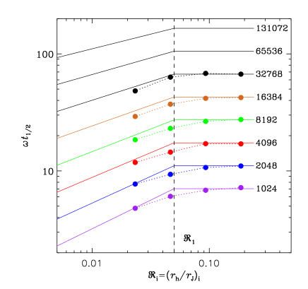
Figure 2: Prediction for the dimensionless half-time, $\omega t_{1/2}$, for clusters in the tidal regime (equation 12) and part of the intermediate regime (§ 3.5) for different $N$. Results of the simulations are shown as dots.

4 Comparison to $N$-body simulations

The results for $\omega t_{1/2}$ of the simulations of clusters with different $N$ and $\mathfrak{R}_{i}$ are presented in Fig. 2. The $\omega t_{1/2}$ results for $\mbox{$\mathfrak{F}$}=0.5$ clusters are nearly the same as those for $\mbox{$\mathfrak{F}$}=1$. For $\mbox{$\mathfrak{F}$}=0.25(0.125)$ the $\omega t_{1/2}$ values are approximately 10%(25%) shorter compared to the Roche-lobe filling results, whereas a scaling with $t_{\rm rh}$ predicts a difference of a factor of $4^{1.5}(8^{1.5})\simeq 8(23)$. From Table 1 we see that clusters that start Roche-lobe under-filling, have evolved for a much larger number of relaxation times than Roche-lobe filling clusters by the time they reach $t_{1/2}$.

5 Conclusions

The dissolution time-scale of clusters evolving in a tidal field, in dimensionless units ($\omega\mbox{$t_{\rm dis}$}$) or in physical units, is almost independent of the initial half-mass radius, $r_{\rm h,i}$, when $r_{\rm h,i}$ relative to the initial Jacobi (or tidal) radius, $r_{\rm J,i}$, is larger than $\mathfrak{R}_{i}(\equiv r_{\rm h,i}/r_{\rm J,i})\gtrsim 0.05$. For clusters that start with $\mathfrak{R}_{i}<0.05$, $t_{\rm dis}$ scales mildly with $\mathfrak{R}_{i}$, between $\mathfrak{R}_{i}^{0.55}$ and $\mathfrak{R}_{i}^{0.35}$ for the range of $N$ we consider and even flatter for larger $N$. Only clusters that start with $\mathfrak{R}_{i}\lesssim 10^{-4}$ can lose half their stars before they reach the influence of the tidal field. We find that in the tidal regime $t_{\rm dis}$ is mainly determined by $N$ and the angular frequency: $\mbox{$t_{\rm dis}$}\propto N^{0.65}/\omega$, that is, what was also found by BM03 for Roche-lobe filling, multi-mass clusters dissolving in tidal fields.

Gnedin & Ostriker (1997) construct the “vital” diagram of globular clusters, which is a triangle in $M$ vs. $r_{\rm h}$ space, outside which clusters should have been destroyed. There are numerous globular clusters with small $r_{\rm h}$ outside this triangle, which the authors denote as lucky survivors. We show that small clusters can in fact survive.

Models that try to explain the evolution of the globular cluster mass function (GCMF) from an initial power-law to a (universal) peaked distribution by stellar dynamical processes are in difficulties, since such models will always produce less dissolution in the outer parts of galaxies. McLaughlin & Fall (2008) have recently proposed a solution to this problem by assuming that $\mbox{$\mbox{${\rm d}$}M/\mbox{${\rm d}$}t$}\propto M/t_{\rm rh}$ and so $\mbox{$\mbox{${\rm d}$}M/\mbox{${\rm d}$}t$}\propto\sqrt{\mbox{$\rho_{\rm h}$}}$ (equations 1&2, with $\xi_{\rm e}$ constant), that is, their $t_{\rm dis}$ is determined by internal relaxation effects only and is independent of the strength of the tidal field. However, our results show that $\xi_{\rm e}$ is not constant and, therefore, $\mbox{${\rm d}$}M/\mbox{${\rm d}$}t$ does not scale as $\sqrt{\mbox{$\rho_{\rm h}$}}$. This makes the universality of the GCMF a problem (again), when trying to explain this by dynamical evolution alone.

References

- Aarseth (1999) Aarseth S. J., 1999, PASP, 111, 1333
- Ambartsumian (1938) Ambartsumian V. A., 1938, Sci. Mem. Leningrade State Univ. #22, ser. Math. Sci. (astronomy), 4, 19
- Baumgardt (2001) Baumgardt H., 2001, MNRAS, 325, 1323 (B01)
- Baumgardt et al. (2002) Baumgardt H., Hut P., Heggie D. C., 2002, MNRAS, 336, 1069
- Baumgardt & Makino (2003) Baumgardt H., Makino J., 2003, MNRAS, 340, 227
- Boutloukos & Lamers (2003) Boutloukos S. G., Lamers H. J. G. L. M., 2003, MNRAS, 338, 717
- Chernoff & Weinberg (1990) Chernoff D. F., Weinberg M. D., 1990, ApJ, 351, 121
- Engle (1999) Engle K. A., 1999, PhD thesis, AA(DREXEL UNIVERSITY)
- Fall & Rees (1977) Fall S. M., Rees M. J., 1977, MNRAS, 181, 37P
- Fukushige & Heggie (2000) Fukushige T., Heggie D. C., 2000, MNRAS, 318, 753
- Gieles et al. (2005) Gieles M., Bastian N., Lamers H. J. G. L. M., Mout J. N., 2005, A&A, 441, 949
- Gieles et al. (2006) Gieles M., Portegies Zwart S. F., Baumgardt H., Athanassoula E., Lamers H. J. G. L. M., Sipior M., Leenaarts J., 2006, MNRAS, 371, 793
- Giersz & Heggie (1994a) Giersz M., Heggie D. C., 1994a, MNRAS, 268, 257
- Giersz & Heggie (1994b) Giersz M., Heggie D. C., 1994b, MNRAS, 270, 298
- Giersz & Heggie (1997) Giersz M., Heggie D. C., 1997, MNRAS, 286, 709
- Gnedin & Ostriker (1997) Gnedin O. Y., Ostriker J. P., 1997, ApJ, 474, 223
- Goodman (1984) Goodman J., 1984, ApJ, 280, 298
- Heggie & Mathieu (1986) Heggie D. C., Mathieu R. D., 1986, in Hut P., McMillan S., eds, Lecture Notes in Physics Vol. 267, The Use of Supercomputers in Stellar Dynamics, Springer-Verlag, Berlin, p.233, 267, 233
- Hénon (1961) Hénon M., 1961, Annales d’Astrophysique, 24, 369
- King (1958) King I., 1958, AJ, 63, 465
- King (1966) King I. R., 1966, AJ, 71, 64
- Lamers et al. (2005a) Lamers H. J. G. L. M., Gieles M., Bastian N., Baumgardt H., Kharchenko N. V., Portegies Zwart S., 2005a, A&A, 441, 117
- Lamers et al. (2005b) Lamers H. J. G. L. M., Gieles M., Portegies Zwart S. F., 2005b, A&A, 429, 173
- Larsen (2004) Larsen S. S., 2004, A&A, 416, 537
- Makino et al. (2003) Makino J., Fukushige T., Koga M., Namura K., 2003, PASJ, 55, 1163
- McLaughlin & Fall (2008) McLaughlin D. E., Fall S. M., 2008, ApJ, 679, 1272
- McMillan & Hut (1996) McMillan S. L. W., Hut P., 1996, ApJ, 467, 348
- Portegies Zwart et al. (2001) Portegies Zwart S., McMillan S. L. W., Hut P., Makino J., 2001, MNRAS, 321, 199
- Scheepmaker et al. (2007) Scheepmaker R. A., Haas M. R., Gieles M., Bastian N., Larsen S. S., Lamers H. J. G. L. M., 2007, A&A, 469, 925
- Spitzer (1987) Spitzer L., 1987, Dynamical evolution of globular clusters. Princeton, NJ, Princeton University Press, 1987, 191 p. (S87)
- Spitzer (1940) Spitzer L. J., 1940, MNRAS, 100, 396
- Spitzer & Chevalier (1973) Spitzer L. J., Chevalier R. A., 1973, ApJ, 183, 565
- Spitzer & Hart (1971) Spitzer L. J., Hart M. H., 1971, ApJ, 164, 399
- Takahashi & Portegies Zwart (2000) Takahashi K., Portegies Zwart S. F., 2000, ApJ, 535, 759