Local Procrustes for Manifold Embedding:
A Measure of Embedding Quality and Embedding Algorithms

Abstract

We present the Procrustes measure, a novel measure based on Procrustes rotation that enables quantitative comparison of the output of manifold-based embedding algorithms (such as LLE (Roweis and Saul, 2000) and Isomap (Tenenbaum et al, 2000)). The measure also serves as a natural tool when choosing dimension-reduction parameters. We also present two novel dimension-reduction techniques that attempt to minimize the suggested measure, and compare the results of these techniques to the results of existing algorithms. Finally, we suggest a simple iterative method that can be used to improve the output of existing algorithms.

1 Introduction

Technological advances constantly improve our ability to collect and store large sets of data. The main difficulty in analyzing such high-dimensional data sets is, that the number of observations required to estimate functions at a set level of accuracy grows exponentially with the dimension. This problem, often referred to as the curse of dimensionality, has led to various techniques that attempt to reduce the dimension of the original data.

Historically, the main approach to dimension reduction is the linear one. This is the approach used by principle component analysis (PCA) and factor analysis (see Mardia et al, 1979, for both). While these algorithms are largely successful, the assumption that a linear projection describes the data well is incorrect for many data sets. A more realistic assumption than that of an underlying linear structure is that the data is on, or next to, an embedded manifold of low dimension in the high-dimensional space. Here a manifold is defined as a topological space that is locally equivalent to a Euclidean space. Locally, the manifold can be estimated by linear approximations based on small neighborhoods of each point. Many algorithms were developed to perform embedding for manifold-based data sets, including the algorithms suggested by Roweis and Saul (2000); Tenenbaum et al (2000); Belkin and Niyogi (2003); Zhang and Zha (2004); Donoho and Grimes (2004); Weinberger and Saul (2006); Dollar et al (2007). Indeed, these algorithms have been shown to succeed even where the assumption of linear structure does not hold. However, to date there exists no good tool to estimate the quality of the result of these algorithms.

Ideally, the quality of an output embedding could be judged based on a comparison to the structure of the original manifold. Indeed, a measure based on the idea that the manifold structure is known to a good degree was recently suggested by Dollar et al (2007). However, in the general case, the manifold structure is not given, and is difficult to estimate accurately. As such ideal measures of quality cannot be used in the general case, an alternate quantitative measure is required.

In this work we suggest an easily computed function that measures the quality of any given embedding. We believe that a faithful embedding is an embedding that preserves the structure of the local neighborhood of each point. Therefore the quality of an embedding is determined by the success of the algorithm in preserving these local structures. The function we present, based on the Procrustes analysis, compares each neighborhood in the high-dimensional space and its corresponding low-dimensional embedding. Theoretical results regarding the convergence of the proposed measure are presented.

We further suggest two new algorithms for discovering the low-dimensional embedding of a high-dimensional data set, based on minimization of the suggested measure function. The first algorithm performs the embedding one neighborhood at a time. This algorithm is extremely fast, but may suffer from incremental distortion. The second algorithm, based on simulated annealing (Kirkpatrick et al, 1983), performs the embedding of all local neighborhoods simultaneously. A simple iterative procedure that improves on an existing output is also presented.

The paper is organized as follows. The problem of manifold learning is presented in Section 2. A discussion regarding the quality of embeddings in general and the suggested measure of quality are presented in Section 3. The embedding algorithms are presented in Section 4. In Section 5 we present numerical examples. All proofs are presented in the Appendix.

2 Manifold-learning problem setting and definitions

In this section we provide a formal definition of the manifold-learning dimension-reduction problem.

Let $\mathcal{M}$ be a $d$-dimensional manifold embedded in $\mathbb{R}^{q}$. Assume that a sample is taken from $\mathcal{M}$. The goal of manifold-learning is to find a faithful embedding of the sample in $\mathbb{R}^{d}$. The assumption that the sample is taken from a manifold is translated to the fact that small distances on the manifold $\mathcal{M}$ can be approximated well by the Euclidian distance in $\mathbb{R}^{q}$. Therefore, to find an embedding, one first needs to approximate the structure of small neighborhoods on the manifold using the Euclidian metric in $\mathbb{R}^{q}$. Then one must find a unified embedding of the sample in $\mathbb{R}^{d}$ that preserves the structure of local neighborhoods on $\mathcal{M}$.

In order to adhere to this scheme, we need two more assumptions. First, we assume that $\mathcal{M}$ is isometrically embedded in $\mathbb{R}^{q}$. By definition, an isometric mapping between two manifolds preserves the inner product on the tangent bundle at each point. Less formally, this means that distances and angles are preserved by the mapping. This assumption is needed because we are interested in an embedding that everywhere preserves the local structure of distances and angles between neighboring points. If this assumption does not hold, close points on the manifold may originate from distant points in $\mathbb{R}^{d}$ and vice versa. In this case, the structure of the local neighborhoods on the manifold will not reveal the structure of the original neighborhoods in $\mathbb{R}^{d}$. We remark here that the assumption that the embedding is isometric is strong but can be relaxed. One may assume instead that the embedding mapping is conformal. This means that the inner products on the tangent bundle at each point are preserved up to a scalar $c$ that may change continuously from point to point. Note that the class of isometric embeddings is included in the class of conformal embeddings. While our main discussion regards isometric embeddings, we will also discuss the conformal embedding problem, which is the framework of algorithms such as c-Isomap (de Silva and Tenenbaum, 2003) and Conformal Embeddings (CE) (Sha and Saul, 2005).

The second assumption is that the sample taken from the manifold $\mathcal{M}$ is dense. We need to prevent the situation in which the local neighborhood of a point, which is computed according to the Euclidian metric in $\mathbb{R}^{q}$, includes distant geodesic points on the manifold. This can happen, for example, if the manifold is twisted. The result of having distant geodesic points in the same local neighborhood is that these distant points will be embedded close to each other instead of preserving the true geodesic distance between them.

To define the problem formally, we require some definitions.

The neighborhood of a point $x_{i}\in\mathcal{M}$ is a set of points $X_{i}$ that consists of points close to $x_{i}$ with respect to the Euclidean metric in $\mathbb{R}^{q}$. For example, neighbors can be $K$-nearest neighbors or all the points in an $\varepsilon$-ball around $x_{i}$.

The minimum radius of curvature $r_{0}=r_{0}(\mathcal{M})$ is defined as follows:

$$\frac{1}{r_{0}}=\max_{\gamma,t}\left\{\left\|\ddot{\gamma(t)}\right\|\right\}$$

where $\gamma$ varies over all unit-speed geodesics in $\mathcal{M}$ and $t$ is in a domain of $\gamma$.

The minimum branch separation $s_{0}=s_{0}(\mathcal{M})$ is defined as the largest positive number for which $\left\|x-\tilde{x}\right\|<s_{0}$ implies $d_{\mathcal{M}}(x,\tilde{x})\leq\pi r_{0}$, where $x,\tilde{x}\in\mathcal{M}$ and $d_{\mathcal{M}}(x,\tilde{x})$ is the geodesic distance between $x$ and $\tilde{x}$ (see Bernstein et al, 2000., for both definitions).

We define the radius $r(i)$ of neighborhood $i$ to be

$$r(i)=\max_{j\in\{1,\ldots,k(i)\}}\left\|x_{i}-x_{i_{j}}\right\|$$

where $x_{i_{j}}$ is the $j$-th out of the $k(i)$ neighbors of $x_{i}$. Finally, we define $r_{\max}$ to be the maximum over $r(i)$ .

We say that the sample is dense with respect to the chosen neighborhoods if $r_{\max}<s_{0}$. Note that this condition depends on the manifold structure, the given sample, and the choice of neighborhoods. However, for a given compact manifold, if the distribution that produces the sample is supported throughout the entire manifold, this condition is valid with probability increasing towards $1$ as the size of the sample is increased and the radius of the neighborhoods is decreased.

We now state the manifold-learning problem more formally. Let $D\subset\mathbb{R}^{d}$ be a compact set and let $\phi:D\rightarrow\mathbb{R}^{q}$ be a smooth and invertible isometric mapping. Let $\mathcal{M}$ be the $d$-dimensional image of $D$ in $\mathbb{R}^{q}$. Let $x_{1},\ldots,x_{n}$ be a sample taken from $\mathcal{M}$. Define neighborhoods $X_{i}$ for each of the points $x_{i}$. Assume that the sample $x_{1},\ldots,x_{n}$ is dense with respect to the choice of $X_{i}$. Find $y_{1},\ldots,y_{n}\in\mathbb{R}^{d}$ that approximate $\phi^{-1}(x_{1}),\ldots,\phi^{-1}(x_{n})$ up to rotation and translation.

3 Faithful embedding

As discussed in Section 2, a faithful embedding should preserve the structure of local neighborhoods on the manifold, while finding a global embedding mapping.

In this section, we will attempt to answer the following two questions:

1. How do we define “preservation of the local structure of a neighborhood”?

2. How do we find a global embedding that preserves the local structure?

We now address the first question. Under the assumption of isometry, it seems reasonable to demand that neighborhoods on the manifold and their corresponding embeddings be closely related. A neighborhood on the manifold and its embedding can be compared using the Procrustes statistic. The Procrustes statistic measures the distance between two configurations of points. The statistic computes the sum of squares between pairs of corresponding points after one of the configurations is rotated and translated to best match the other.

In the remainder of this paper we will represent any set of $k$ points $x_{1},\ldots,x_{k}\in\mathbb{R}^{q}$ as a matrix $X_{k\times q}=[x_{1}^{\prime},\ldots,x_{k}^{\prime}]$; i.e., the $j$-th row of the matrix $X$ corresponds to $x_{j}$.

Let $X$ be a $k$-point set in $\mathbb{R}^{q}$ and let $Y$ be a $k$-point set in $\mathbb{R}^{d}$, where $d\leq q$. We define the Procrustes statistic $G(X,Y)$ as

$$G(X,Y) = \inf_{\{A,b:\,A^{\prime}A=I,\,b\in\mathbb{R}^{q}\}}\sum_{i=1}^{k}\left\|x_{i}-Ay_{i}-b\right\|^{2}$$

$$= \inf_{\{A,b:\,A^{\prime}A=I,\,b\in\mathbb{R}^{q}\}}\textrm{tr}\left((X-YA^{\prime}-1b^{\prime})^{\prime}(X-YA^{\prime}-1b^{\prime})\right)$$

where the rotation matrix $A$ is a columns-orthogonal $q\times d$ matrix, $A^{\prime}$ is the adjoint of $A$, and $1$ is a $k$-dimensional vector of ones.

The Procrustes rotation matrix $A$ and the Procrustes translation vector $b$ that minimize $G(X,Y)$ can be computed explicitly, as follows. Let $Z=X^{\prime}HY$ where $H\equiv I-\frac{1}{k}11^{\prime}$ is the centering matrix. Let $ULV^{\prime}$ be the singular-value decomposition (svd) of $Z$, where $U$ is an orthogonal $q\times d$ matrix, $L$ is a non-negative $d\times d$ diagonal matrix, and $V$ is a $d\times d$ orthogonal matrix (Mardia et al, 1979). Then, the Procrustes rotation matrix $A$ is given by $UV^{\prime}$ (Sibson, 1978). The Procrustes translation vector $b$ is given by $\bar{x}-A\bar{y}$, where $\bar{x}$ and $\bar{y}$ are the sample means of $X$ and $Y$, respectively. Due to the last fact, we may write $G(X,Y)$ without the translation vector $b$ as

$$G(X,Y)=\inf_{\{A:\,A^{\prime}A=I\}}\textrm{tr}\left((X-YA^{\prime})^{\prime}H(X-YA^{\prime})\right)=\inf_{\{A:\,A^{\prime}A=I\}}\left\|H(X-YA^{\prime})\right\|_{F}^{2}\,,$$

where $\left\|\,\right\|_{F}$ is the Frobenius norm.

Given $X$, the minimum of $G(X,Y)$ can be computed explicitly and is achieved by the first $d$ principal components of $X$. This result is a consequence of the following lemma.

Lemma 1

Let $X=X_{k\times q}$ be a centered matrix of rank $q$ and let $d\leq q$. Then

$$\inf_{\{\tilde{X}:\,\mathrm{rank}(\tilde{X})=d\}}\|X-\tilde{X}\|^{2}_{F}$$ (2)

is obtained when $\tilde{X}$ equals the projection of $X$ on the subspace spanned by the first $d$ principal components of $X$.

For proof, see Mardia et al (1979, page 220).

Returning to the questions posed at the beginning of this section, we will define how well an embedding preserves the local neighborhoods using the Procrustes statistic $G(X_{i},Y_{i})$ of each neighborhood-embedding pair $(X_{i},Y_{i})$. Therefore, a global embedding that preserves the local structure can be found by minimizing the sum of the Procrustes statistics of all neighborhood-embedding pairs.

More formally, let $X$ be the $q$-dimensional sample from the manifold and let $Y$ be a $d$-dimensional embedding of $X$. Let $X_{i}$ be the neighborhood of $x_{i}$ ($i=1,\dots,n$) and $Y_{i}$ its embedding. Define

$$R(X,Y)=\frac{1}{n}\sum_{i=1}^{n}G(X_{i},Y_{i})\;.$$ (3)

The function $R$ measures the average quality of the neighborhood embeddings. Embedding $Y$ is considered better than embedding $\tilde{Y}$ in the local-neighborhood-preserving sense if $R(X,Y)<R(X,\tilde{Y})$. This means that on the average, $Y$ preserves the structure of the local neighborhoods better than $\tilde{Y}$.

The function $R(X,Y)$ is sensitive to scaling, therefore normalization should be considered. A reasonable normalization is

$$R_{N}(X,Y)=\frac{1}{n}\sum_{i=1}^{n}G(X_{i},Y_{i})/\left\|HX_{i}\right\|_{F}^{2}\,.$$ (4)

The $i$-th summand of $R_{N}(X,Y)$ examines how well the rotated and translated $Y_{i}$ “explains” $X_{i}$, independent of the size of $X_{i}$. This normalization solves the problem of increased weighting for larger neighborhoods that exists in the unnormalized $R(X,Y)$. It also allows comparison of embeddings for data sets of different sizes. Hence, this normalized version is used to compare the results of different outputs (see Section 5).

In the remainder of this section, we will justify our choice of the Procrustes measure $R$ for a quantitative comparison of embeddings. We will also present two additional, closely related measures. One measure is $R_{PCA}$, which can ease computation when the input space is of high dimension. The second measure is $R_{C}$, which is a statistic designed for conformal mappings (see Section 2). Finally, we will discuss the relation between the measures suggested in this work to the objective functions of other algorithms, namely LTSA (Zhang and Zha, 2004) and SDE (Weinberger and Saul, 2006).

We now justify the use of the Procrustes statistic $G(X_{i},Y_{i})$ as a measure of the quality of the local embedding. First, $G(X_{i},Y_{i})$ estimates the relation between the entire input neighborhood and its embedding as one entity, instead of comparing angles and distances within the neighborhood with those within its embedding. Second, the Procrustes statistic is not highly sensitive to small perturbations of the embedding. More formally, $G(X,Y)=\mathcal{O}(\varepsilon^{2})$, where $Y=X+\varepsilon Z$ and $Z$ is a general matrix (see Sibson, 1979). Finally, the function $G$ is $l_{2}$-norm-based and therefore prefers small differences at many points to big differences at fewer points. This is preferable in our context, as the local embedding of the neighborhood should be compatible with the embeddings of nearby neighborhoods.

The usage of $R$ as a measure of the quality of the global embedding of the manifold is justified by Theorem 3.1. Theorem 3.1 claims that when the number of input points $X$ increases, the low-dimensional points $Z=\phi^{-1}(X)$ of the input data tend to zero $R$. This implies that the minimizer $Y$ of $R$ should be close to the original data set $Z$ (up to rotation and translation).

Theorem 3.1

Let $\mathcal{D}$ be a compact connected set. Let $\phi:\mathcal{D}\rightarrow\mathbb{R}^{q}$ be an isometry. Let $X^{(n)}$ be an $n$-point sample taken from $\phi(\mathcal{D})$, and let $Z^{(n)}=\phi^{-1}(X^{(n)})$. Assume that the sample $X^{(n)}$ is dense with respect to the choice of neighborhoods for all $n\geq N_{0}$. Then for all $n\geq N_{0}$

$$R\left(X^{(n)},Z^{(n)}\right)=\mathcal{O}(r_{max}^{4})\,.$$ (5)

See Appendix A.1 for proof.

Replacing $R(X,Y)$ with the normalized version $R_{N}(X,Y)$ (see Eq. 4) and noting that $\left\|HX_{i}\right\|_{F}^{2}=\mathcal{O}(r_{i}^{2})$, we obtain

Corollary 1

$$R_{N}(X^{(n)},Z^{(n)})=\mathcal{O}(r_{max}^{2})\,.$$

To avoid heavy computations, a slightly different version of $R(X,Y)$ can be considered. Instead of measuring the difference between the original neighborhoods on the manifold and their embeddings, one can compare the local PCA projections (Mardia et al, 1979) of the original neighborhoods with their embeddings. We therefore define

$$R_{PCA}(X,Y)=\frac{1}{n}\sum_{i=1}^{n}G(X_{i}P_{i},Y_{i})\,,$$ (6)

where $P_{i}$ is the $d$-dimensional PCA projection matrix of $X_{i}$.

The convergence theorem for $R_{PCA}$ is similar to Theorem 3.1, but the convergence is slower.

Theorem 3.2

Let $\mathcal{D}$ be a compact connected set. Let $\phi:\mathcal{D}\rightarrow\mathbb{R}^{q}$ be an isometry. Let $X^{(n)}$ be an $n$-point sample taken from $\phi(\mathcal{D})$, and let $Z^{(n)}=\phi^{-1}(X^{(n)})$. Assume that the sample $X^{(n)}$ is dense with respect to the choice of neighborhoods for all $n\geq N_{0}$. Then for all $n\geq N_{0}$

$$R_{PCA}\left(X^{(n)},Z^{(n)}\right)=\mathcal{O}(r_{max}^{3})\,,$$

See Appendix A.2 for proof.

We now present another version of the Procrustes measure $R_{C}(X,Y)$, suitable for conformal mappings. Here we want to compare between each original neighborhood $X_{i}$ and its corresponding embedding $Y_{i}$, where we allow $Y_{i}$ not only to be rotated and translated but also to be rescaled. Define

$$G_{C}(X,Y)=\inf_{\{A:\,A^{\prime}A=I,0<c\in\mathbb{R}\}}\textrm{tr}\left(\left(X-Y(cA^{\prime})\right)^{\prime}H\left(X-Y(cA^{\prime})\right)\right)\,.$$

Note that the scalar $c$ was introduced here to allow scaling of $Y$. Let $Z=X^{\prime}HY$ and let $ULV^{\prime}$ be the svd of $Z$. The minimizer rotation matrix $A$ is given by $UV^{\prime}$. The minimizer constant $c$ is given by $\textrm{tr}\left(L\right)/\textrm{tr}\left(Y^{\prime}Y\right)$(see Sibson, 1978). The (normalized) conformal Procrustes measure is given by

$$R_{C}(X,Y)=\frac{1}{n}\sum_{i=1}^{n}G_{C}(X_{i},Y_{i})/\left\|HX_{i}\right\|_{F}^{2}\,.$$ (7)

Note that $R_{C}(X,Y)\leq R_{N}(X,Y)$ since the constraints are relaxed in the definition of $R_{C}(X,Y)$. However, the lower bound in both cases is equal (see Lemma 1).

We present a convergence theorem, similar to that of $R$ and $R_{PCA}$.

Theorem 3.3

Let $\mathcal{D}$ be a compact connected set. Let $\tilde{\phi}:\mathcal{D}\rightarrow\mathbb{R}^{q}$ be a conformal mapping. Let $X^{(n)}$ be an $n$-point sample taken from $\tilde{\phi}(\mathcal{D})$, and let $Z^{(n)}=\tilde{\phi}^{-1}(X^{(n)})$. Assume that the sample $X^{(n)}$ is dense with respect to the choice of neighborhoods for all $n\geq N_{0}$. Then for all $n\geq N_{0}$ we have

$$R_{C}\left(X^{(n)},Z^{(n)}\right)=\mathcal{O}(r_{max}^{2})\,.$$

See Appendix A.3 for proof. Note that this result is of the same convergence rate as of $R_{N}$ (see Corollary 1).

A cost function somewhat similar to the measure $R_{PCA}$ was presented by Zhang and Zha (2004) in a slightly different context. The local PCA projection of neighborhoods was used as an approximation of the tangent plane at each point. The resulting algorithm, local tangent subspaces alignment (LTSA), is based on minimizing the function

$$\sum_{i=1}^{n}\left\|(I-P_{i}P_{i}^{\prime})HY_{i}\right\|_{F}^{2}\,,$$

where the $k(i)\times d$ matrices $P_{i}$ are as in $R_{PCA}$. The minimization performed by LTSA is under a normalization constraint. This means that as a measure, LTSA’s objective function is designed to compare normalized outputs $Y$ (otherwise $Y=0$ would be the trivial minimizer) and is therefore unsuitable as a measure.

Another algorithm worth mentioning here is SDE (Weinberger and Saul, 2006). The constraints on the output required by this algorithm are that all the distances and angles within each neighborhood be preserved. Therefore the output of this algorithm should always be close to the minimum of $R(X,Y)$. The maximization of the objective function of this algorithm

$$\sum_{i,j}\left\|y_{i}-y_{j}\right\|^{2}$$

is reasonable when the aforementioned constraints are enforced. However, it is not relevant as a measure for comparison of general outputs that do not fulfill these constraints.

In summary, we return to the questions posed at the beginning of this section. We choose to define preservation of local neighborhoods as minimization of the Procrustes measure $R$ (see Eq. 3). We therefore find a global embedding that best preserves local structure by minimizing $R$. For computational reasons, minimization of $R_{PCA}$ (see Eq. 6) may be preferred. For conformal maps we suggest the measure $R_{C}$ (see Eq. 7), which allows separate scaling of each neighborhood.

4 Algorithms

In Section 3 we showed that a faithful embedding should yield low $R(X,Y)$ and $R_{PCA}(X,Y)$ values. Therefore we may attempt to find a faithful embedding by minimizing these functions. However, $R(X,Y)$ and $R_{PCA}(X,Y)$ are not necessarily convex functions and may have more than one local minimum. In this section we present two algorithms for minimization of $R(X,Y)$ or $R_{PCA}(X,Y)$. In addition, we present an iterative method that can improve the output of the two algorithms, as well as other existing algorithms.

The first algorithm, greedy Procrustes (GP), performs the embeddings one neighborhood at a time. The first neighborhood is embedded using the PCA projection (see Lemma 1). At each stage, the following neighborhood is embedded by finding the best embedding with respect to the embeddings already found. This greedy algorithm is presented in Section 4.1.

The second algorithm, Procrustes subspaces alignment (PSA), is based on an alignment of the local PCA projection subspaces. The use of local PCA produces a good low-dimensional description of the neighborhoods, but the description of each of the neighborhoods is in an arbitrary coordinate system. PSA performs the global embedding by finding the local embeddings and then aligning them. PSA is described in Section 4.2. Simulated annealing (SA) is used to find the alignment of the subspaces (see Section 4.3).

After an initial solution is found using either GP or PSA, the solution can be improved using an iterative procedure until there is no improvement (see Section 4.4).

4.1 Greedy Procrustes (GP)

GP finds the neighborhoods’ embeddings one by one. The flow of the algorithm is described below.

1. Initialization:

   • Find the neighbors $X_{i}$ of each point $x_{i}$ and let $\mathrm{Neighbors}(i)$ be the indices of the neighbors $X_{i}$.

   • Initialize the list of all embedded points’ indices to $N:=\emptyset$.

2. Embedding of the first neighborhood:

   • Choose an index $i$ (randomly).

   • Calculate the embedding $Y_{i}=X_{i}P_{i}$, where $P_{i}$ is the PCA projection matrix of $X_{i}$.

   • Update the list of indices of embedded points $N=\mathrm{Neighbors}(i)$.

3. Find all other embeddings (iteratively):

   • Find $j$, where $x_{j}$ is the unembedded point with the largest number of embedded neighbors,
     $j=\operatornamewithlimits{argmax}_{p\notin N}\left|\{\mathrm{Neighbors}(p)\cap N\}\right|$.

   • Define $\overline{X}_{j}=\left\{x_{p}|p\in\mathrm{Neighbors}(j)\cap N\right\}$, the points in $X_{j}$ that are already embedded.
     Define $\overline{Y}_{j}$ as the (previously calculated) embedding of $\overline{X}_{j}$.
     Define $\widetilde{X}_{j}=\left\{x_{p}|p\in\mathrm{Neighbors}(j)\setminus N\right\}$, the points in $X_{j}$ that are not embedded yet.

   • Compute the Procrustes rotation matrix $A_{j}$ and translation vector $b_{j}$ between $\overline{X}_{j}$ and $\overline{Y}_{j}$.

   • Define the embedding of the points in $\widetilde{X}_{j}$ as $\widetilde{Y}_{j}=\widetilde{X}_{j}A_{j}+b_{j}$.

   • Update the list of indices of embedded points $N$
     $N:=N\cup\mathrm{Neighbors}(j)$.

4. Stopping condition:
   Stop when $|N|=n$, i.e., when all points are embedded.

The main advantage of GP is that it is fast. The embedding for $X_{i}$ is computed in $\mathcal{O}(k(i)^{3})$ where $k(i)$ is the size of $X_{i}$. Therefore, the overall computation time is $\mathcal{O}(nK^{3})$, where $K=\max_{i}k(i)$. While GP does not claim to find the global minimum, it does find an embedding that preserves the local neighborhood’s structure. The main disadvantage of GP is that it has incremental errors.

4.2 Procrustes Subspaces Alignment (PSA)

$R(X,Y)$ can be written in terms of the Procrustes rotation matrices $A_{i}$ as

$$R(X,Y) = \frac{1}{n}\sum_{i=1}^{n}\inf_{\{A_{i}:\,A_{i}^{\prime}A_{i}=I\}}\left\|H(X_{i}-Y_{i}A_{i}^{\prime})\right\|_{F}^{2}\,,$$

where $H$ is the centering matrix. $A_{i}$ can be calculated, given $X$ and $Y$. However, as $Y$ is not given, one way to find $Y$ is by first guessing the matrices $A_{i}$ and then finding the $Y$ that minimizes

$$R(X,Y|A_{1},\ldots,A_{n})=\frac{1}{n}\sum_{i=1}^{n}\left\|H(X_{i}-Y_{i}A_{i}^{\prime})\right\|_{F}^{2}\,.$$ (8)

$Y$ can be found by taking derivatives of $R(X,Y|A_{1},\ldots,A_{n})$.

We therefore need to choose $A_{i}$ wisely. The choice of the Jacobian matrices $J_{i}\equiv J_{\phi}(z_{i})$ as a guess for $A_{i}$ is justified by the following, as shown in the proof of Theorem 3.1 (see Eq. A.1). As the size of the sample is increased, $\frac{1}{n}\sum_{i=i}^{n}\left\|H(X_{i}-Z_{i}J_{i}^{\prime})\right\|\rightarrow 0$. This means that choosing $J_{i}$ will lead to a solution $Y$ that is close to the minimizer of $R(X,Y)$.

The PCA projection matrices $P_{i}$ approximate the unknown Jacobian matrices $J_{i}$ up to a rotation. To use them in place of $J_{i}$, we must first align the projections correctly. Therefore, our guess for $A_{i}$ is of the form $A_{i}=P_{i}O_{i}$, where $O_{i}$ are $d\times d$ rotation matrices that minimize

$$f(A_{1},\ldots,A_{n})=\sum_{i=1}^{n}\sum_{j\in\mathrm{Neighbors}(i)}\left\|A_{i}-A_{j}\right\|_{F}^{2}\,.$$ (9)

The rotation matrices $O_{i}$ can be found using simulated annealing, as described in Section 4.3.

Once the matrices $A_{i}$ are found, we need to minimize $R(X,Y|A_{1},\ldots,A_{n})$. We first write $R(X,Y|A_{1},\ldots,A_{n})$ in matrix notation as

$$R(X,Y|A_{1},\ldots,A_{n})=\frac{1}{n}\sum_{i=1}^{n}\mathrm{tr}\left((X-YA_{i}^{\prime})^{\prime}H_{i}(X-YA_{i}^{\prime})\right)\,.$$

Here $H_{i}$ is the centering matrix of neighborhood $X_{i}$

$$H_{i}(k,l)=\left\{\begin{array}[]{cc}1-\frac{1}{k(i)}&k=l\mathrm{\,and\,}k\in\mathrm{Neighbors}(i)\\ -\frac{1}{k(i)}&k\neq l\mathrm{\,and\,}k,l\in\mathrm{Neighbors}(i)\\ 0&\mathrm{elsewhere}\,.\end{array}\right.$$

The rows of the matrix $H_{i}X$ at $\mathrm{Neighbors}(i)$ indices are $x_{i}$’s centered neighborhood, where all the other rows equal zero, and similarly for $H_{i}Y$. .

Taking the derivative of $R(X,Y|A_{1},\ldots,A_{n})$ (Eq. 8) with respect to $Y$ (see Mardia et al, 1979) and using the fact that $A_{i}^{\prime}A_{i}=I$, we obtain

$$\frac{\partial}{\partial Y}R(X,Y|A_{1},\ldots,A_{n})=\frac{2}{n}\sum_{i=1}^{n}H_{i}XA_{i}-\frac{2}{n}\sum_{i=1}^{n}H_{i}Y\,.$$ (10)

Using the general inverse of $\sum_{i=1}^{n}H_{i}$ we can write $Y$ as

$$Y=\Big{(}\sum_{i=1}^{n}H_{i}\Big{)}^{\bot}\sum_{i=1}^{n}H_{i}XA_{i}\,.$$ (11)

Summarizing, we present the PSA algorithm.

1. Initialization:

   • Find the neighbors $X_{i}$ of each point $x_{i}$.

   • Find the PCA projection matrices $P_{i}$ of the neighborhood $X_{i}$.

2. Alignment of the projection matrices:
   Find $A_{i}$ that minimize Eq. 9 using, for example, simulated annealing (see Section 4.3).

3. Find the embedding:
   Compute $Y$ according to Eq. 11.

The advantage of this algorithm is that it is global. The computation time of this algorithm (assuming that the matrices $A_{i}$ are already known) depends on multiplying by the inverse of the sparse symmetric semi-positive definite matrix $\sum_{i=1}^{n}H_{i}$, which can be very costly. However, this matrix need not be computed explicitly. Instead, one may solve $d$-linear-equation systems of the form $(\sum_{i=1}^{n}H_{i})x=b$, which can be computed much faster (see, for example, Munksgaard, 1980).

4.3 Simulated Annealing (SA) alignment procedure

In step 2. of PSA (see Section 4.2), it is necessary to align the PCA projection matrices $P_{i}$. In the following we suggest an alignment method based on simulated annealing (SA) (Kirkpatrick et al, 1983). The aim of the suggested algorithm is to find a set of columns-orthonormal matrices $A_{1},\ldots,A_{n}$ that minimize Eq. 9. A number of closely-related algorithms, designed to find embeddings using alignment of some local dimensionally-reduced descriptions, were previously suggested. Roweis et al (2001) and Verbeek et al (2002) introduced algorithms based on probabilistic mixtures of local FA and PCA structures, respectively. As Eq. 9 and these two algorithms suffer from local minima, the use of simulated annealing may be beneficial. Another algorithm, suggested by Teh and Roweis (2003), uses a convex objective function to find the alignment. The output matrices of this algorithm are not necessarily columns-orthonormal, as is required in our case .

Minimizing Eq. 9 is similar to the Ising model problem (see, for example, Cipra, 1987). The Ising model consists of a neighbor-graph and a configuration space that is the set of all possible assignments of $+1$ or $-1$ to each vertex of the graph. A low-energy state is one in which neighboring points have the same sign. Our problem consists of a neighbor-graph with a configuration space that includes all of the rotations of the projection matrices $P_{i}$ at each point $x_{i}$. Minimizing the function $f$ is similar to finding a low-energy state of the Ising model. As solutions to the Ising model usually involve algorithms such as simulated annealing , we take the same path here.

We present the SA algorithm, following the algorithm suggested by Siarry et al (1997), modified for our problem.

1. Initialization:

   • Choose an initial configuration (for example, using GP).

   • Compute the initial temperature (see Siarry et al, 1997).

   • Define the cooling scheme (see Siarry et al, 1997).

2. Single SA step:

   • Choose $i$ randomly.
     Generate a random $d\times d$ rotation matrix $O_{i}$ (see Stewart, 1980).
     Define $A_{i}^{\mathrm{New}}\equiv A_{i}O_{i}$.

   • Compute $f(A_{1},\ldots,A_{i}^{\mathrm{New}},\ldots,A_{n})$.
     Note that it is enough to compute $\sum_{\mathrm{Neighbors}(i)}\left\|A_{i}^{\mathrm{New}}-A_{j}\right\|_{F}^{2}$.

   • Accept $A_{i}^{\mathrm{New}}$ if either

     $$f(A_{1},\ldots,A_{i}^{\mathrm{New}},\ldots,A_{n})<f(A_{1},\ldots,A_{i},\ldots,A_{n})$$

     or with some probability depending on the current temperature.

   • Decrease the temperature and stop if the lowest temperature is reached.

3. Outer iterations:

   • First iteration: Perform a run of SA on all matrices $A_{1},\ldots,A_{n}$.
     Find the largest cluster of aligned matrices (for example, use BFS (Corman et al, 1990) and define an alignment criterion).

   • Other iterations: Apply SA to the matrices that are not in the largest cluster. Update the largest cluster after each run.

   • Repeat until the size of the largest cluster includes almost all of the matrices $A_{i}$.

Using SA is complicated. The cooling scheme requires the estimation of many parameters, and the run-time depends heavily on the correct choice of these parameters. For output of large dimension, the alignment is difficult, and the output of SA can be poor. Although SA is a time-consuming algorithm, each iteration is very simple, involving only $O(Kqd^{3})$ operations, where $K$ is the maximum number of neighbors, and $q$ and $d$ are the input and output dimensions, respectively. In addition, the memory requirements are modest. Therefore, SA can run even when the number of points is large.

4.4 Iterative procedure

Given a solution of GP, PSA, or any other technique, it is usually possible to modify $Y$ so that $R(X,Y)$ is further decreased. The idea of the iterative procedure we present here was suggested independently by Zhang and Zha (2004), but no details were supplied.

In Section 4.2, we showed that given $Y$, the improved matrices $A_{i}$ are obtained by finding the Procrustes matrices between $Y_{i}$ and $X_{i}$. Given the matrices $A_{i}$, the embedding $Y$ can be found using Eq. 11. An iterative procedure would require finding first the new matrices $A_{i}$ and then a new embedding $Y$ at each stage. This would be repeated until the change in the value of $R(X,Y)$ was small.

The problem with this scheme is that it involves the computation of the inverse of the matrix $\sum_{i=1}^{n}H_{i}$ (see end of Section 4.2). We therefore suggest a modified version of this iterative procedure, which is easier to compute. Recall that

$$R(X,Y)=\sum_{i=1}^{n}\sum_{j\in\mathrm{Neighbors}(i)}\left\|x_{j}-A_{i}y_{j}-b_{i}\right\|^{2}\,.$$

The least-squares solution for $b_{i}$ is

$$\frac{1}{|\{\mathrm{Neighbors}(i)\}|}\sum_{j\in\mathrm{Neighbors}(i)}\left(x_{j}-A_{i}y_{j}\right)\,.$$ (12)

The least-squares solution for $y_{j}$ is

$$\frac{1}{|\{i:j\in\mathrm{Neighbors}(i)\}|}\sum_{\{i:j\in\mathrm{Neighbors}(i)\}}A_{i}^{\prime}(x_{j}-b_{i})\,.$$ (13)

Note that we get a different solution than that in Eq. 10. The reason is that here we consider $b_{i}$ as constants when we look for a solution for $y_{j}$. In fact, $y_{j}$ appear in the definition of the $b_{i}$. However, as $y_{j}$ appear there multiplied by $1/k(i)$, these terms make only a small contribution.

We suggest performing the iterations as follows. First, find the Procrustes rotation matrices $A_{i}$ and the translation vectors $b_{i}$ using Eq. 12. Then find $y_{j}$ using Eq. 13. Repeat until $R(X,Y)$ no longer decreases significantly.

5 Numerical Examples

In this section we evaluate the algorithms GP and PSA on data sets that we assumed to be sampled from underlying manifolds. We compare the results to those obtained by LLE (Roweis and Saul, 2000), Isomap (Tenenbaum et al, 2000), and LTSA (Zhang and Zha, 2004), both visually and using the measures $R_{N}(X,Y)$ and $R_{C}(X,Y)$ (see Table 2).

The algorithms GP and PSA were implemented in the Matlab environment, running on a Pentium 4 with a 3 Ghz CPU and 0.98 GB of RAM. The alignment stage of PSA was implemented using SA (see Section 4.3). The runs of both GP and PSA were followed by the iterative procedure described in Section 4.4 to improve the minimization of $R(X,Y)$. LLE, Isomap, and LTSA were evaluated using the Matlab code taken from the sites of the respective authors. The algorithm SDE (Weinberger and Saul, 2006), whose minimization is closest in spirit to ours, was also tested; however, it suffers from heavy computational demands, and the results of this algorithm could not be obtained using the code provided in the site.

The data sets are described in Table 1. We ran all five algorithms using $k=6,9,12,15$ and $18$ nearest neighbors. The minimum values for $R_{N}(X,Y)$ and $R_{C}(X,Y)$ are presented in Table 2. The results in all cases were qualitatively the same, therefore in the images we show the results for $k=12$ only.

Name	n	q	d	Description	Figure
Swissroll	1600	3	2	isometrically embedded in $R^{3}$	Fig 1
Hemisphere	2500	3	2	not isometrically embedded	Fig 2
				in $R^{3}$
Cylinder	800	3	2	locally isometric to $R^{2}$,	Fig 3
				has no global embedding in $R^{2}$
Faces	1965	560	3	$20\times 28$ pixel grayscale face images	Fig 4
				(see Roweis, retrieved Nov. 2006)
Twos	638	256	10	images of handwritten “2”s	None,due
				from the USPS data set	to output
				of handwritten digits (Hull, 1994)	dimension

Table 1: Description of five data sets used to compare the different algorithms. $n$ is the sample size and $q$ and $d$ are the input and output dimensions, respectively.

Overall, GP and PSA perform satisfactorily as shown both in the figures and in Table 2. The fact that in most of the examples GP and PSA get lower values than LLE, Isomap, and LTSA is perhaps not surprising, as GP and PSA are designed to minimize $R(X,Y)$. The run-times of the algorithms excluding PSA is on the order of seconds while it takes PSA a few hours to run. Memory requirements of GP and PSA are lower than those of the other algorithms. As a consequence of the memory requirements, results could not be obtained for LLE, Isomap and LTSA for $n>3000$.

Use of the measure $R(X,Y)$ allows a quantitative comparison of visually similar outputs. Regarding the output of the cylinder (see Fig. 3), for example, PSA and Isomap both give topologically sound results; however, $R(X,Y)$ shows that locally, PSA does a better job. In addition, $R(X,Y)$ can be used to optimize embedding parameters such as neighborhood size (see Fig.5).

	Swissroll	Hemisphere	Cylinder	Faces	Twos
GP	0.00 [0.00]	0.02 [0.01]	0.13 [0.01]	0.45 [0.36]	0.00 [0.00]
PSA	0.00 [0.00]	0.03 [0.01]	0.02 [0.01]	0.35 [0.30	0.00 [0.00]
LLE	0.81 [0.23]	0.60 [0.00]	0.73 [0.13]	0.99 [0.79]	0.82 [0.23]
Isomap	0.01 [0.01]	0.03 [0.02]	0.34 [0.25]	0.5 [0.38]	0.02 [0.01]
LTSA	0.99 [0.22]	0.93 [0.04]	0.59 [0.48]	0.99 [0.53]	0.98 [0.37]
Lower Bound	0.00	0.00	0.00	0.11	0.00

Table 2: Comparison of the output of the different algorithms using $R_{N}(X,Y)\;[R_{C}(X,Y)]$ as the measures of the quality of the embeddings. These values are the minima of both measures as a function of neighborhood size $k$, for $k=6,9,12,15,18$. The lower bound was computed using local PCA at each neighborhood (see Lemma 1).

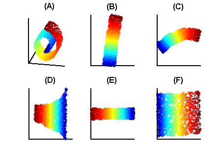
Figure 1: A $1600$-point sample taken from the three-dimensional Swissroll input is presented in (A). (B)-(F) show the output of GP, PSA, LLE, Isomap, and LTSA, respectively, for $k=12$. Both GP and PSA, like Isomap, succeed in finding the proportions of the original data.

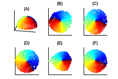
Figure 2: The input of a $2500$-point sample taken from a hemisphere is presented in (A). (B)-(F) show the output of GP, PSA, LLE, Isomap, and LTSA, respectively, for $k=12$. Both GP and PSA, like the other algorithms, perform the embedding, although the assumption of isometry does not hold for the hemisphere.

Figure 3: The input of an $800$-point sample taken from a cylinder is presented in (A). (B)-(F) show the output of GP, PSA, LLE, Isomap, and LTSA, respectively, for $k=12$. Note that the cylinder has no embedding in $\mathbb{R}^{2}$ and it is not clear what is the best embedding in this case. While PSA, Isomap, and LLE succeeded in finding the topological ring structure of the cylinder, only PSA and LLE succeed in preserving the width of the cylinder. GP and LTSA collapse the cylinder and therefore fail to find the global structure, though they preform well for most of the neighborhoods (see Table 2).

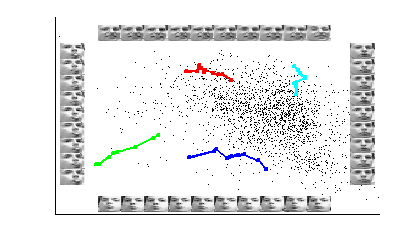
Figure 4: The projection of the three-dimensional output, as computed by PSA, on the first two coordinates (small points). The input used was a $1965$-point sample of grayscale images of faces (see Table 1). The boxes connected by lines are nearby points in the output set. The images are the corresponding face images from the input, in the same order. We see that nearby images in the input space correspond to nearby points in the output space.

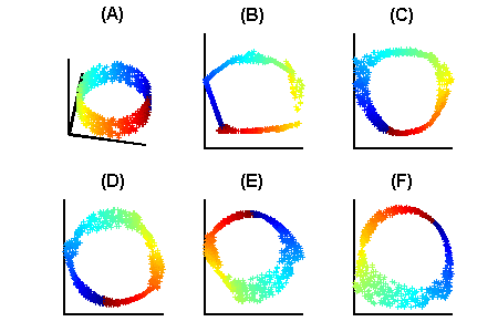
Figure 5: The input of an $800$-point sample taken from a cylinder is presented in (A). (B)-(F) show the output of LLE for $k=6,9,12,15$ and $18$, respectively. The respective values of $R_{C}(X,Y)$ are $0.25,\,0.15,\,0.13,\,0.19,\,0.17$. While qualitatively the results are similar, $R_{C}(X,Y)$ indicates that $k=12$ is optimal.

6 Discussion

In this section, we emphasize the main results of this work and indicate possible directions for future research.

We demonstrated that overall, the measure $R(X,Y)$ provides a good estimation of the quality of the embedding. It allows a quantitative comparison of the outputs of various embedding algorithms. Moreover, it is quickly and easily computed. However, two points should be noted.

First, $R(X,Y)$ measures only the local quality of the embedding. As emphasized in Fig. 3, even outputs that do not preserve the global structure of the input may yield relatively low $R$-values if the local neighborhood structure is generally preserved. This problem is shared by all manifold-embedding techniques that try to minimize only local attributes of the data. The problem can be circumvented by adding a penalty for outputs that embed distant geodesic points close to each other. Distant geodesic points can be defined, for example, as points at least $s$-distant on the neighborhood graph, with $s>1$.

Second, $R(X,Y)$ is not an ideal measure of the quality of embedding for algorithms that normalize their output, such as LLE (Roweis and Saul, 2000), Laplacian Eigenmap (Belkin and Niyogi, 2003), and LTSA (Zhang and Zha, 2004). This is because normalization of the output distorts the structure of the local neighborhoods and therefore yields high $R$-values even if the output seems to find the underlying structure of the input. This point (see also discussion in Sha and Saul, 2005, Section 2) raises the questions, which qualities are preserved by these algorithms and how can one quantify these qualities. However, it is clear that these algorithms do not perform faithful embedding in the sense defined in Section 3. The measure $R_{C}(X,Y)$ addresses this problem to some degree, by allowing separate scaling of each neighborhood (see Table 2). One could consider an even more relaxed measure which allows not only rotation, translations and scaling but a general linear transformation of each neighborhood. However, it is not clear what exactly such measure would quantify. Two new embedding algorithms were introduced. We discuss some aspects of these algorithms below.

PSA, in the form we suggested in this work, uses SA to align the tangent subspaces at all points. While PSA works reasonably well for small input sets and low output dimension spaces, it is not suitable for large data sets. However, the algorithm should not be rejected as a whole. Rather, a different or modified technique for subspaces alignment, for example the use of landmarks (de Silva and Tenenbaum, 2003), is required in order to make this algorithm truly useful.

GP is very fast ($\mathcal{O}(n)$ where $n$ is the number of sample points), can work on very large input sets (even $100,000$ in less than an hour), and obtains good results as shown both in Figs. 1-4 and in Table 2. This algorithm is therefore an efficient alternative to the existing algorithms. It may also be used to choose optimal parameters, such as neighborhood size and output dimension, before other algorithms are applied. $R(X,Y)$ can be used for the comparison of GP outputs for varied parameters.

An important issue that was not considered in depth in this paper is that of noisy input data. The main problem with noisy data is that, locally, the data seems $q$-dimensional, even if the manifold is $d$-dimensional, $d<q$. To overcome this problem, one should choose neighborhoods that are large relative to the magnitude of the noise, but not too large with respect to the curvature of the manifold. If the neighborhood size is chosen wisely, both PSA and GP should overcome the noise and perform the embedding well (see Fig. 6). This is due to the fact that both algorithms are based on Procrustes analysis and PCA, which are relatively robust against noise. Further study is required to define a method for choosing the optimal neighborhood size.

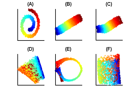
Figure 6: The profile of noisy input of a $2500$-point sample taken from a swissroll is presented in (A). (B)-(F) show the output of GP, PSA, LLE, Isomap and LTSA respectively. Note that only GP and PSA succeed to find the structure of the swissroll.

Appendix A Proofs

A.1 Proof of Theorem 3.1

In this section, we denote the points of neighborhood $X_{i}$ as $x_{i_{1}},\ldots,x_{i_{k(i)}}$, where $k(i)$ is the number of neighbors in $X_{i}$.

Proof

In order to prove that $R(X,Z)=\frac{1}{n}\sum_{i=1}^{n}G(X_{i},Z_{i})$ is $\mathcal{O}(r_{\max}^{4})$, it is enough to show that for each $i\in 1,\ldots,n$, $G(X_{i},Z_{i})=\mathcal{O}(r_{i}^{4})$, where $r_{i}$ is the radius of the $i$-th neighborhood. The proof consists of replacing the Procrustes rotation matrix $A_{i}$ by $J_{i}\equiv J_{\phi}(z_{i})$, the Jacobian of the mapping $\phi$ at $z_{i}$. Note that the fact that $\phi$ is an isometry ensures that $J_{i}^{\prime}J_{i}=I$. The Procrustes translation vector $b_{i}$ is replaced by $x_{i}-J_{i}z_{i}$.

Recall that by definition $x_{j}-x_{i}=\phi(z_{j})-\phi(z_{i})$; therefore $x_{j}-x_{i}=J_{i}(z_{i}-z_{j})+\mathcal{O}\left(\left\|z_{j}-z_{i}\right\|^{2}\right)$. Hence,

$$G(X_{i},Z_{i}) = \inf_{A_{i},b_{i}}\sum_{j=1}^{k(i)}\left\|x_{i_{j}}-A_{i}z_{i_{j}}-b_{i}\right\|^{2}$$

$$\leq \sum_{j=1}^{k(i)}\left\|x_{i_{j}}-J_{i}z_{i_{j}}-(x_{i}-J_{i}z_{i})\right\|^{2}$$

$$= \sum_{j=1}^{k(i)}\left\|(x_{i_{j}}-x_{i})-J_{i}(z_{i_{j}}-z_{i})\right\|^{2}$$

$$= \sum_{j=1}^{k(i)}\mathcal{O}\left(\left\|z_{i_{j}}-z_{i}\right\|^{4}\right)\,.$$

$\phi$ is an isometry, therefore $d_{\mathcal{M}}(x_{i_{j}},x_{i})=\left\|z_{i_{j}}-z_{i}\right\|$, where $d_{\mathcal{M}}$ is the geodesic metric. The sample is assumed to be dense, hence $\left\|x_{i_{j}}-x_{i}\right\|<s_{0}$, where $s_{0}$ is the minimum branch separation (see Section 2). Using Bernstein et al (2000., Lemma 3) we conclude that

$$\left\|z_{i_{j}}-z_{i}\right\|=d_{\mathcal{M}}(x_{i_{j}},x_{i})<\frac{\pi}{2}\left\|x_{i_{j}}-x_{i}\right\|\,.$$

We can therefore write $\mathcal{O}\left(\left\|z_{i_{j}}-z_{i}\right\|^{4}\right)=\mathcal{O}(r_{i}^{4})$, which completes the proof.

A.2 Proof of Theorem 3.2

The proof of Theorem 3.2 is based on the idea that the PCA projection matrix $P_{i}$ is usually a good approximation of the span of the Jacobian $J_{i}$. The structure of the proof is as follows. First we quantify the relations between $X_{i}P_{i}$ and $X_{i}J_{i}$, the projections of the $i$-th neighborhood using the PCA projection matrix and the Jacobian, respectively. Then we follow the lines of the proof of Theorem 3.1, using the bounds obtained previously.

To compare the PCA projection subspace and tangent subspace at $x_{i}$ we use the notation of angle between subspaces. Note that both subspaces are $d$-dimensional and are embedded in the Euclidian space $\mathbb{R}^{q}$. The columns of the matrices $P_{i}$ and $J_{i}$ consist of orthonormal bases of the PCA projection space and of the tangent space, respectively. Denote these subspaces by $\mathcal{P}_{i}$ and $\mathcal{J}_{i}$, respectively. Surprisingly, the angle between $\mathcal{P}_{i}$ and $\mathcal{J}_{i}$ can be arbitrarily large. However, in the following we show that even if the angle between the subspaces is large, the projected neighborhoods are close.

We start with some definitions. The principal angles $\sigma_{1},\ldots,\sigma_{d}$ between $\mathcal{J}_{i}$ and $\mathcal{P}_{i}$ may be defined recursively for $p=1,\dots,d$ as (see Golub and Loan, 1983)

$$\cos(\sigma_{p})=\max_{v\in\mathcal{P}_{i}}\max_{w\in\mathcal{J}_{i}}v^{\prime}w\,,$$

subject to

$$\left\|v\right\|=\left\|w\right\|=1,\;v^{\prime}v_{k}=0,w^{\prime}w_{k}=0\;;k=1,\ldots,p-1\,.$$

The vectors $v_{1},\ldots,v_{d}$ and $w_{1},\ldots,w_{d}$ are called principal vectors.

The fact that $P_{i}$ and $J_{i}$ have orthogonal columns leads to a simple way to calculate the principal vectors and angles explicitly. Let $ULV^{\prime}$ be the svd of $J_{i}^{\prime}P_{i}$. Then (see Golub and Loan, 1983)

1. $v_{1},\ldots,v_{d}$ are given by the columns of $P_{i}V$.

2. $w_{1},\ldots,w_{d}$ are given by the columns of $J_{i}U$.

The relations between the two sets of vectors plays an important role in our computations. Write $w_{p}=\alpha_{p}v_{p}+\beta_{p}v_{p}^{\perp}$, where $\alpha_{p}=w_{p}^{\prime}v_{p}$, $\beta_{p}=\left\|w_{p}-\alpha_{p}v_{p}\right\|$ and $v_{p}^{\perp}=\frac{w_{p}-\alpha_{p}v_{p}}{\left\|w_{p}-\alpha_{p}v_{p}\right\|}$. Note that $\alpha_{p}$ is the cosine of the $p$-th principal angle between $\mathcal{P}_{i}$ and $\mathcal{J}_{i}$. The angle between the subspaces is defined as $\arccos(\alpha_{d})$ and the distance between the two subspaces is defined to be $\sin(\alpha_{d})$.

We now prove some basic claims related to the principal vectors.

Lemma 2

Let $P_{i}$ be the projection matrix of the neighborhood $X_{i}$ and let $J_{i}$ be the Jacobian of $\phi$ at $z_{i}$. Let $ULV^{\prime}$ be the svd of $J_{i}^{\prime}P_{i}$ and $v_{1},\ldots,v_{d}$ and $w_{1},\ldots,w_{d}$ be the columns of $P_{i}V$ and $J_{i}U$, respectively. Then

1. $v_{1},\ldots,v_{d}$ are an orthonormal vector system.

2. $w_{1},\ldots,w_{d}$ are an orthonormal vector system.

3. $v_{p}\perp w_{q}$ for $p\neq q$.

4. $v_{p}^{\perp}\perp v_{q}^{\perp}$ for $p\neq q$.

5. $v_{p}^{\perp}\perp v_{q}$ for $q=1,\ldots,d$.

Proof

1. True, since $P_{i}V$ is an orthonormal matrix.

2. True, since $J_{i}U$ is an orthonormal matrix.

3. Note that $(J_{i}U)^{\prime}(P_{i}V)=U^{\prime}(J_{i}^{\prime}P_{i})V=L$ where $L$ is a diagonal non-negative matrix.

4. $$(\beta_{p}v_{p}^{\perp})^{\prime}(\beta_{q}v_{q}^{\perp}) = (w_{p}-\alpha_{p}v_{p})^{\prime}(w_{q}-\alpha_{p}v_{q})$$

   $$= w_{p}^{\prime}w_{q}-v_{p}{}^{\prime}w_{q}-v_{q}^{\prime}w_{p}+v_{p}{}^{\prime}v_{q}=0\,.$$

5. $$(\beta_{p}v_{p}^{\perp})^{\prime}v_{q} = (w_{p}-\alpha_{p}v_{p})^{\prime}v_{q}$$

   $$= w_{p}^{\prime}v_{q}-\alpha_{p}v_{p}{}^{\prime}v_{q}$$

   $$= \delta_{pq}\alpha_{p}-\delta_{pq}\alpha_{p}=0\,.$$

Using the relation between the principal vectors, we can compare the description of the neighborhood $X_{i}$ in the local PCA coordinations and its description in the tangent space coordinations. Here we need to exploit two main facts. The first fact is that the local PCA projection of a neighborhood is the best approximation, in the $l_{2}$ sense, to the original neighborhood. Specifically, it is a better approximation than the tangent space in the $l_{2}$ sense. The second is that in a small neighborhood of $x_{i}$, the tangent space itself is a good approximation to the original neighborhood. Formally, the first assertion means that

$$\sum_{j=1}^{k(i)}\left\|(x_{i_{j}}-\bar{x}_{i})\right\|^{2}\geq\sum_{j=1}^{k(i)}\left\|P_{i}^{\prime}(x_{i_{j}}-\bar{x}_{i})\right\|^{2}\geq\sum_{j=1}^{k(i)}\left\|J_{i}^{\prime}(x_{i_{j}}-\bar{x}_{i})\right\|^{2}$$ (15)

while the second assertion means that

$$\sum_{j=1}^{k(i)}\left\|(x_{i_{j}}-\bar{x}_{i})\right\|^{2}-\sum_{j=1}^{k(i)}\left\|J_{i}^{\prime}(x_{i_{j}}-\bar{x}_{i})\right\|^{2}=\mathcal{O}(r_{i}^{4})\,.$$ (16)

The proof of Eq. 16 is straightforward. First note that

$$(x_{i_{j}}-\bar{x}_{i}) = (x_{i_{j}}-x_{i})-(\bar{x}_{i}-x_{i})$$

$$= J_{i}(z_{i_{j}}-z_{i})-J_{i}(\bar{z}_{i}-z_{i})+\mathcal{O}(r_{i}^{2})$$

$$= J_{i}(z_{i_{j}}-\bar{z}_{i})+\mathcal{O}(r_{i}^{2})\,.$$

Hence

$$\left\|(x_{i_{j}}-\bar{x}_{i})\right\|^{2}-\left\|J_{i}^{\prime}(x_{i_{j}}-\bar{x}_{i})\right\|^{2} = \sum_{p=d+1}^{q}(w_{p}^{\prime}(x_{i_{j}}-\bar{x}_{i}))^{2}$$

$$= \left\|(x_{i_{j}}-\bar{x}_{i})-J_{i}J_{i}^{\prime}(x_{i_{j}}-\bar{x}_{i})\right\|^{2}$$

$$= \left\|J_{i}(z_{i_{j}}-\bar{z}_{i})-J_{i}J_{i}^{\prime}(J_{i}(z_{i_{j}}-\bar{z}_{i}))+\mathcal{O}(r_{i}^{2})\right\|^{2}$$

$$= \left\|\mathcal{O}(r_{i}^{2})\right\|^{2}=\mathcal{O}(r_{i}^{4})\,,$$

where $w_{d+1},\ldots,w_{q}$ are a completion of $w_{1},\ldots,w_{d}$ to an orthonormal basis of $\mathbb{R}^{q}$ and we used the fact that $J_{i}^{\prime}J_{i}=I$.

The following is a lemma regarding the relations between the PCA projection matrix and the Jacobian projection. It is a consequence of Eq. 15.

Lemma 3

1. $\sum_{j=1}^{k(i)}\left\|(x_{i_{j}}-\bar{x}_{i})\right\|^{2}-\sum_{j=1}^{k(i)}\left\|V^{\prime}P_{i}^{\prime}(x_{i_{j}}-\bar{x}_{i})\right\|^{2}=\mathcal{O}(r_{i}^{4})$.

2. $\sum_{j=1}^{k(i)}\left\|V^{\prime}P_{i}^{\prime}(x_{i_{j}}-\bar{x}_{i})\right\|^{2}-\sum_{j=1}^{k(i)}\left\|U^{\prime}J_{i}^{\prime}(x_{i_{j}}-\bar{x}_{i})\right\|^{2}=\mathcal{O}(r_{i}^{4})$.

3. $(x_{i_{j}}-\bar{x}_{i})^{\prime}v_{p}=\mathcal{O}(r_{i})$.

4. $(x_{i_{j}}-\bar{x}_{i})^{\prime}v_{p}^{\perp}=\mathcal{O}(r_{i}^{2})$.

Proof

1. and 2. follow from Eqs. 15 and 16.

2. follows from the definition of $r_{i}$.

3. is a consequence of 1., indeed,

   $$\sum_{j=1}^{k(i)}\sum_{p=1}^{d}\left(v_{p}^{\perp}{}^{\prime}(x_{i_{j}}-\bar{x}_{i})\right)^{2} \leq \sum_{j=1}^{k(i)}\left\|(x_{i_{j}}-\bar{x}_{i})\right\|^{2}-\sum_{j=1}^{k(i)}\left\|V^{\prime}P_{i}^{\prime}(x_{i_{j}}-\bar{x}_{i})\right\|^{2}$$

   $$= \mathcal{O}(r_{i}^{4})\,.$$

We now prove Theorem 3.2. Similarly to the proof of Theorem 3.1, it is enough to show that $G(X_{i}P_{i},Z_{i})=\mathcal{O}(r_{i}^{3})$.

$$G(X_{i}P_{i},Z_{i}) = \inf_{A_{i},b_{i}}\sum_{j=1}^{k(i)}\left\|P_{i}^{\prime}x_{i_{j}}-A_{i}z_{i_{j}}-b_{i}\right\|^{2}$$

$$\leq \sum_{j=1}^{k(i)}\left\|P_{i}^{\prime}(x_{i_{j}}-\bar{x}_{i})-O_{i}(z_{i_{j}}-\bar{z}_{i})\right\|^{2}$$

$$= \sum_{j=1}^{k(i)}\left\|P_{i}^{\prime}(x_{i_{j}}-\bar{x}_{i})-O_{i}J_{i}^{\prime}(x_{i_{j}}-\bar{x}_{i})+O_{i}J_{i}^{\prime}(x_{i_{j}}-\bar{x}_{i})-O_{i}(z_{i_{j}}-\bar{z}_{i})\right\|^{2}$$

$$\leq \sum_{j=1}^{k(i)}\left\|P_{i}^{\prime}(x_{i_{j}}-\bar{x}_{i})-O_{i}J_{i}^{\prime}(x_{i_{j}}-\bar{x}_{i})\right\|^{2}+\sum_{j=1}^{k(i)}\left\|O_{i}J_{i}^{\prime}(x_{i_{j}}-\bar{x}_{i})-O_{i}(z_{i_{j}}-\bar{z}_{i})\right\|^{2}$$

$$\equiv \mathrm{Exp1}+\mathrm{Exp2}\,,$$

where $O_{i}$ is some $d\times d$ orthogonal matrix. Note that due to its orthogonality, Exp2 is independent of the specific choice of $O_{i}$.

We choose $O_{i}=VU^{\prime}$. Rewriting $\mathrm{Exp1}$ we obtain

$$\mathrm{Exp1} = \sum_{j=1}^{k(i)}\left\|P_{i}^{\prime}(x_{i_{j}}-\bar{x}_{i})-O_{i}J_{i}^{\prime}(x_{i_{j}}-\bar{x}_{i})\right\|^{2}$$

$$= \sum_{j=1}^{k(i)}\left\|P_{i}^{\prime}(x_{i_{j}}-\bar{x}_{i})-VU^{\prime}J_{i}^{\prime}(x_{i_{j}}-\bar{x}_{i})\right\|^{2}$$

$$= \sum_{j=1}^{k(i)}\left\|V^{\prime}P_{i}^{\prime}(x_{i_{j}}-\bar{x}_{i})-(V^{\prime}V)U^{\prime}J_{i}^{\prime}(x_{i_{j}}-\bar{x}_{i})\right\|^{2}$$

$$= \sum_{j=1}^{k(i)}\sum_{p=1}^{d}\left(v_{p}{}^{\prime}(x_{i_{j}}-\bar{x}_{i})-w_{p}^{\prime}(x_{i_{j}}-\bar{x}_{i})\right)^{2}\,.$$

This last expression brings out the difference between the description of the neighborhood $X_{i}$ in the local PCA coordinations and its description in the tangent space coordinates. Using Lemma 2, we can write

$$\mathrm{Exp1} = \sum_{j=1}^{k(i)}\sum_{p=1}^{d}\big{(}(v_{p}-w_{p})^{\prime}(x_{i_{j}}-\bar{x}_{i})\big{)}^{2}$$

$$= \sum_{j=1}^{k(i)}\sum_{p=1}^{d}\big{(}v_{p}-\alpha_{p}v_{p}-\beta_{p}v_{p}^{\perp})^{\prime}(x_{i_{j}}-\bar{x}_{i})\big{)}^{2}$$

$$= \sum_{j=1}^{k(i)}\sum_{p=1}^{d}\ (1-\alpha_{p})^{2}\big{(}v_{p}{}^{\prime}(x_{i_{j}}-\bar{x}_{i})\big{)}^{2}$$

$$-\sum_{j=1}^{k(i)}\sum_{p=1}^{d}2(1-\alpha_{p})\beta_{p}\big{(}v_{p}{}^{\prime}(x_{i_{j}}-\bar{x}_{i})\big{)}\big{(}v_{p}^{\perp}{}^{\prime}(x_{i_{j}}-\bar{x}_{i})\big{)}$$

$$+\sum_{j=1}^{k(i)}\sum_{p=1}^{d}\beta_{p}^{2}\big{(}v_{p}^{\perp}{}^{\prime}(x_{i_{j}}-\bar{x}_{i})\big{)}^{2}\,.$$

We will use Lemma 3 to bound the first expression of the RHS.

$$\mathcal{O}(r_{i}^{4}) = \sum_{j=1}^{k(i)}\left\|V^{\prime}P_{i}^{\prime}(x_{i_{j}}-\bar{x}_{i})\right\|^{2}-\sum_{j=1}^{k(i)}\left\|U^{\prime}J_{i}^{\prime}(x_{i_{j}}-\bar{x}_{i})\right\|^{2}$$

$$= \sum_{j=1}^{k(i)}\sum_{p=1}^{d}\Big{\{}\big{(}v_{p}{}^{\prime}(x_{i_{j}}-\bar{x}_{i})\big{)}^{2}-\big{(}(\alpha_{p}v_{p}+\beta_{p}v_{p}^{\perp})^{\prime}(x_{i_{j}}-\bar{x}_{i})\big{)}^{2}\Big{\}}$$

$$= \sum_{j=1}^{k(i)}\sum_{p=1}^{d}(1-\alpha_{p}^{2})\big{(}v_{p}{}^{\prime}(x_{i_{j}}-\bar{x}_{i})\big{)}^{2}$$

$$+2\sum_{j=1}^{k(i)}\sum_{p=1}^{d}\alpha_{p}\beta_{p}\big{(}v_{p}{}^{\prime}(x_{i_{j}}-\bar{x}_{i})\big{)}\big{(}v_{p}^{\perp}{}^{\prime}(x_{i_{j}}-\bar{x}_{i})\big{)}$$

$$-\sum_{j=1}^{k(i)}\sum_{p=1}^{d}\beta_{p}^{2}\big{(}v_{p}^{\perp}{}^{\prime}(x_{i_{j}}-\bar{x}_{i})\big{)}^{2}\,.$$

Note also that $(1-\alpha_{p})^{2}\leq 1-\alpha_{p}^{2}$. Hence,

$$\sum_{j=1}^{k(i)}\sum_{p=1}^{d}\ (1-\alpha_{p})^{2}\big{(}v_{p}{}^{\prime}(x_{i_{j}}-\bar{x}_{i})\big{)}^{2} \leq \sum_{j=1}^{k(i)}\sum_{p=1}^{d}\beta_{p}^{2}\big{(}v_{p}^{\perp}{}^{\prime}(x_{i_{j}}-\bar{x}_{i})\big{)}^{2}$$

$$-2\sum_{j=1}^{k(i)}\sum_{p=1}^{d}\alpha_{p}\beta_{p}\big{(}v_{p}{}^{\prime}(x_{i_{j}}-\bar{x}_{i})\big{)}\big{(}v_{p}^{\perp}{}^{\prime}(x_{i_{j}}-\bar{x}_{i})\big{)}$$

$$+\mathcal{O}(r_{i}^{4})\,.$$

Plugging it into Eq. A.2 we get

$$\mathrm{Exp1} \leq \sum_{j=1}^{k(i)}\sum_{p=1}^{d}2\beta_{p}^{2}\big{(}v_{p}^{\perp}{}^{\prime}(x_{i_{j}}-\bar{x}_{i})\big{)}^{2}$$

$$-\sum_{j=1}^{k(i)}\sum_{p=1}^{d}2\beta_{p}\big{(}v_{p}{}^{\prime}(x_{i_{j}}-\bar{x}_{i})\big{)}\big{(}v_{p}^{\perp}{}^{\prime}(x_{i_{j}}-\bar{x}_{i})\big{)}+\mathcal{O}(r_{i}^{4})$$

$$\leq \mathcal{O}(r_{i}^{4})+\mathcal{O}(r_{i}^{3})+\mathcal{O}(r_{i}^{4})=\mathcal{O}(r_{i}^{3})\,,$$

where the last inequality is due to Lemma 3.

Proving that Exp2 is $\mathcal{O}(r_{i}^{4})$ is straightforward.

$$\mathrm{Exp2} = \sum_{j=1}^{k(i)}\left\|O_{i}J_{i}^{\prime}(x_{i_{j}}-\bar{x}_{i})-O_{i}(z_{i_{j}}-\bar{z}_{i})\right\|^{2}$$

$$= \sum_{j=1}^{k(i)}\left\|J_{i}^{\prime}(x_{i_{j}}-\bar{x}_{i})-(z_{i_{j}}-\bar{z}_{i})\right\|^{2}=\mathcal{O}(r_{i}^{4})\,,$$

which concludes the proof of Theorem 3.2.

A.3 Proof of Theorem 3.3

The proof is similar to the proof of Theorem 3.1 (see Section A.1). The proof consists of replacing the Procrustes rotation matrix $A_{i}$ and the constant $c_{i}$ by $J_{i}\equiv J_{\tilde{\phi}}(z_{i})$, the Jacobian of the mapping $\tilde{\phi}$ at $z_{i}$. Note that as $\tilde{\phi}$ is an conformal mapping which ensures that $J_{i}^{\prime}J_{i}=cI$. The Procrustes translation vector $b_{i}$ is replaced by $x_{i}-J_{i}z_{i}$.

Recall that by definition $x_{j}-x_{i}=\tilde{\phi}(z_{j})-\tilde{\phi}(z_{i})$; therefore $x_{j}-x_{i}=J_{i}(z_{i}-z_{j})+\mathcal{O}\left(\left\|z_{j}-z_{i}\right\|^{2}\right)$. Hence,

$$G(X_{i},Z_{i}) = \inf_{A_{i},b_{i},c_{i}}\sum_{j=1}^{k(i)}\left\|x_{i_{j}}-c_{i}A_{i}z_{i_{j}}-b_{i}\right\|^{2}$$

$$\leq \sum_{j=1}^{k(i)}\left\|x_{i_{j}}-J_{i}z_{i_{j}}-(x_{i}-J_{i}z_{i})\right\|^{2}$$

$$= \sum_{j=1}^{k(i)}\mathcal{O}\left(\left\|z_{i_{j}}-z_{i}\right\|^{4}\right)\,.$$

As $\tilde{\phi}$ is an conformal mapping, we have $c_{\min}\left\|z_{i_{j}}-z_{i}\right\|\leq d_{\mathcal{M}}(x_{i_{j}},x_{i})$, where $d_{\mathcal{M}}$ is the geodesic metric and $c_{\min}>0$ is the minimum of the scale function $c(z)$ measures the scaling change of $\phi$ at $z$ . The minimum $c_{\min}$ is attained as $\mathcal{D}$ is compact. The last inequality holds true since the geodesic distance $d_{\mathcal{M}}(x_{i_{j}},x_{i})$ equals to the integral over $c(z)$ for some path between $z_{i_{j}}$ and $z_{i}$.

The sample is assumed to be dense, hence $\left\|x_{i_{j}}-x_{i}\right\|<s_{0}$, where $s_{0}$ is the minimum branch separation (see Section 2). Using again Bernstein et al (2000., Lemma 3) we conclude that

$$\left\|z_{i_{j}}-z_{i}\right\|\leq\frac{1}{c_{\min}}d_{\mathcal{M}}(x_{i_{j}},x_{i})<\frac{\pi}{2c_{\min}}\left\|x_{i_{j}}-x_{i}\right\|\,.$$

We can therefore write $\mathcal{O}\left(\left\|z_{i_{j}}-z_{i}\right\|^{4}\right)=\mathcal{O}(r_{i}^{4})$. Dividing by the normalization $\left\|HX_{i}\right\|_{F}^{2}$ for each neighborhood we obtain $R_{C}(X,Y)=\mathcal{O}(r_{\max}^{2})$ which completes the proof.