A New Approach for Reconstructing SUSY Particle Masses with a few $\rm fb^{-1}$ at the LHC

Abstract

We describe a new cascade mass reconstruction approach to allow reconstruction of SUSY particle masses in long cascades (five or more particles) at the LHC with integrated luminosity as low as a few $\rm fb^{-1}$. This approach is based on a consecutive use of the endpoint method, an event filter and a combinatorial mass reconstruction method. The endpoint method gives a preliminary estimate of light sparticle masses. An event filter combining the maximum likelihood distributions for all events in the data sample allows suppression of backgrounds and gives a preliminary estimate of heavy sparticle masses. Finally, SUSY particle masses are reconstructed by a search for a maximum of a combined likelihood function constructed for each possible combination of five events in the data sample.

SUSY data sample sets for the SU3 model point containing 80k events each were generated, corresponding to an integrated luminosity of 4.2 $\rm fb^{-1}$. These events were passed through the AcerDET detector simulator, which parametrized the response of a detector. To demonstrate the stability and precision of the approach five different 80k event data sets were considered. Masses were reconstructed with a precision of about $10\%$ for heavy sparticles and $10-20\%$ for light sparticles.

I. Introduction

Supersymmetry [1] is a very popular extension of the Standard Model. By introducing an equal number of fermion and boson degrees of freedom SUSY leads to a cancellation of quadratic divergences in the Higgs sector and provides an attractive solution to the hierarchy problem [2]. If supersymmetry exists at an energy scale of  1 TeV, the production cross sections of SUSY particles can be significant and effects of SUSY particles should be observed at the LHC, which should reach an integrated luminosity of 300 $\rm fb^{-1}$ in about 5 years [3]. In many supersymmetric models, in order to avoid undesirable weak scale proton decay, R-parity conservation is assumed. This leads to pair production of SUSY particles and therefore the lightest SUSY particle (LSP) is stable. As a result, SUSY events at an accelerator will give two decay chains, each containing one LSP and Standard Model particles in the final state. The reconstruction of a SUSY event is complicated because of escaping LSPs and many complex and competing decay modes. In this paper we will consider mass reconstruction of five SUSY particles in the cascade decay

$$\tilde{g}\to\tilde{b}b_{2}\to\tilde{\chi}_{2}^{0}b_{1}b_{2}\to\tilde{l}_{R}l_{2}b_{1}b_{2}\to\tilde{\chi}_{1}^{0}l_{1}l_{2}b_{1}b_{2}$$ (1)

The gluino decay chain (1) is shown in Fig.(1)

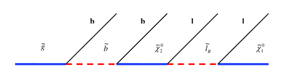
Figure 1: A gluino cascade decay chain.

At present there are two different approaches to SUSY mass reconstruction. The standard technique for analysis is “the endpoint method” which has been widely studied [3] - [10] for high integrated luminosity of about $100-300~{}\rm fb^{-1}$ at the LHC. This method looks for kinematic endpoints. SUSY particle masses are reconstructed by minimizing the $\chi^{2}$ function of the difference between observed and theoretical endpoints.

The second method of SUSY particle mass reconstruction is the so called “mass relation method” [11],[12] based on the mass relation equation (see Appendix A) which relates SUSY particle masses and measured momenta of detected particles. The “mass relation equation” is obtained as a solution of a system of four-momentum constraints for each vertex in the decay chain (1). For example for the gluino decay vertex it follows that $m_{\tilde{g}}^{2}=(p_{\tilde{\chi}_{1}^{0}}+k_{l_{1}}+k_{l_{2}}+p_{b_{1}}+p_{b_{2}})^{2}$ which give the relation between four components of LSP four-momentum in terms of decaying particle mass, LSP mass and the four-momenta of detectable particles. Similar relations can be obtained for each vertex in the process (1). There are four vertices in the cascade (1) so one gets four kinematic equations that can be solved for four components of LSP four-momentum in terms of SUSY masses and momenta of detectable particles. By substituting these components into the on-shell mass condition for LSP $m_{\tilde{\chi}_{1}^{0}}^{2}=p_{\tilde{\chi}_{1}^{0}}^{2}$ the “mass relation equation” including all SUSY masses ($\vec{m}$) and detectable particle momenta ($\vec{p}$) in the process (1)

$$f(\vec{m},\vec{p})=0$$ (2)

is found (an explicit form of this equation is given in Appendix A). This equation is valid for any SUSY event including the cascade (1). For one event this equation is underconstrained, it contains five unknown masses.

Authors of  [12] developed two approaches to the problem of mass search at high luminosity of about $300~{}\rm fb^{-1}$. Both approaches assumed that three light SUSY particle masses ($\tilde{\chi}_{2}^{0}$, $\tilde{l}_{R}$, and $\tilde{\chi}_{1}^{0}$) are known. In this case, the mass relation equation contains only two unknown parameters, the masses of the heaviest sparticles. In the first “event pair analysis” approach it was assumed that SUSY particles are the same from event to event. Gluino and bottom squark masses are reconstructed in this case by solving the system of two mass relation equations. The second approach is based on the search for the maximum of the combined likelihood function for all events which is constructed by an individual likelihood function for each event taking into account the mass relation equation in two dimensional $(m_{\tilde{g}},m_{\tilde{b}})$ mass space. The search for the maximum of the combined likelihood function allows reconstruction of gluino and bottom squark masses at high integrated luminosity.

We note that the reconstruction at low integrated luminosity (with a few $\rm fb^{-1}$) does not work for heavy sparticle masses for either “the endpoint method” and “the mass relation method” in their original forms.

“The endpoint method” uses only events near the end point; therefore, high statistics is required. Also, in order to reconstruct the gluino mass a non-relativistic approximation is used for the LSP near the end point. This approximation is not justified for situations with $\tilde{l}_{R}$ close in mass either to $\tilde{\chi}_{2}^{0}$ or $\tilde{\chi}_{1}^{0}$. Note that in [9] an approach was proposed to obtain the gluino mass without a non-relativistic approximation.

“Pair analysis” of “the mass relation method” assumes that masses of SUSY particles are the same from event to event while in reality heavy particle masses follow a Breit-Wigner distribution. Therefore, an attempt to extend this approach to five masses often leads to an inconsistent system of equations or wrong solutions. An attempt to extend the original combined likelihood function approach [12] based on a grid search in five dimensions leads to unreasonably intensive computing calculations.

The goal of the present article is to develop an approach allowing reconstruction all of five masses of the cascade (1) at low integrated luminosity of a few $\rm fb^{-1}$. This luminosity can be reached at the early stage of the LHC in comparison with a projected integrated luminosity of $300~{}\rm fb^{-1}$ in five years. This approach is based on a consecutive use of the endpoint method, an event filter and a combinatorial mass reconstruction method. It was found that reliable results are obtained only with a good starting point for the final fit and by rejecting a large fraction of the background. The first two methods are used to define five SUSY particle mass ranges for the final combinatorial mass reconstruction method in which all five masses are simultaneously fit and allowed to vary from event to event. The endpoint method therefore is used to get a preliminary estimation of the light SUSY particle ($\tilde{\chi}_{2}^{0},\tilde{l}_{R},\tilde{\chi}_{1}^{0}$) masses and corresponding errors. These masses are then used with the mass relation equation constraint to construct the maximum likelihood distribution in the two heaviest-sparticle mass-plane for each individual event. An event filter combining the maximum likelihood distributions for all events in the data sample allows determination of the range of heavy ($\tilde{g},\tilde{b}$) masses and significant suppression of the background. Finally SUSY particle masses are reconstructed by a search for a maximum of a combined likelihood function, which depends on all five sparticle masses, constructed for each possible combination of five events in the data sample. The approach is self-contained; no information on the nature of the data set (SU3, SPS1a or other) is used.

Note that a possible way to improve “the mass relation method” was proposed in [13] by considering all events at the same time and fitting all five masses simultaneously.

II.Simulation

We choose for this study the SU3 model point. This point has a significant production cross section for the chain (1): gluinos and squarks should be produced abundantly at the LHC. The bulk point SU3 is the official benchmark point of the ATLAS collaboration and it is in agreement with the recent precision WMAP data  [14]. This model point is described by the set of mSUGRA [15] parameters given in Table (1).

Point	$m_{0}$	$m_{1/2}$	$A_{0}$	$tan\beta$	$\mu$
SU3	100 GeV	300 GeV	-300 GeV	6	$>$ 0

Table 1: mSUGRA parameters for the SU3 point.

Branching ratios for the gluino decay chain (1) at the SU3 point are

$$\tilde{g}\stackrel{{\scriptstyle 16.6\%}}{{\longrightarrow}}\tilde{b}_{1}\stackrel{{\scriptstyle 24.1\%}}{{\longrightarrow}}\tilde{\chi}_{2}^{0}\stackrel{{\scriptstyle 11.4\%}}{{\longrightarrow}}\tilde{l}_{R}\stackrel{{\scriptstyle 100\%}}{{\longrightarrow}}\tilde{\chi}_{1}^{0}~{}~{}\Rightarrow~{}~{}0.46\%$$

$$\tilde{g}\stackrel{{\scriptstyle 9.2\%}}{{\longrightarrow}}\tilde{b}_{2}\stackrel{{\scriptstyle 16.6\%}}{{\longrightarrow}}\tilde{\chi}_{2}^{0}\stackrel{{\scriptstyle 11.4\%}}{{\longrightarrow}}\tilde{l}_{R}\stackrel{{\scriptstyle 100\%}}{{\longrightarrow}}\tilde{\chi}_{1}^{0}~{}~{}\Rightarrow~{}~{}0.18\%$$

Assumed theoretical masses of SUSY particles in the cascade (1), the total branching ratio and a cross section generated by ISAJET 7.74 are given in Table (2).

Point	$m_{\tilde{g}}$	$m_{\tilde{b_{1}}}$	$m_{\tilde{b}_{2}}$	$m_{\tilde{\chi}_{2}^{0}}$	$m_{\tilde{l}_{R}}$	$m_{\tilde{\chi}_{1}^{0}}$	BR	$\sigma[\rm pb]$
SU3	720.16	605.93	642.00	223.27	154.63	118.83	0.64$\%$	19

Table 2: Assumed theoretical masses of sparticles, branching ratio BR and production cross section $\sigma$ at the SU3 point. Masses are given in GeV.

Monte Carlo simulations of SUSY production at model points were performed by the HERWIG 6.510 event generator  [16]. The produced events were passed through the AcerDET detector simulation  [17], which parametrized the response of a detector. Samples of 80k SUSY events were used. This approximately corresponds to $4.2~{}\rm fb^{-1}$ of integrated luminosity because the SUSY production cross section is 19 pb at the SU3 point. Five different sets of 80k SUSY events were considered to demonstrate the stability and precision of the mass reconstruction approach.

In order to isolate the chain (1) the following standard cuts were applied:

$\bullet$ two isolated opposite-sign same-flavor (OSSF) leptons (not tau leptons) satisfying transverse momentum cuts $p_{T}(l^{\pm})>20~{}GeV$ and $p_{T}(l^{\mp})>10~{}GeV$

$\bullet$ two b-tagged jets with $p_{T}>50~{}GeV$;

$\bullet$ At least three jets, the hardest satisfying $p_{T1}>150~{}GeV$, $p_{T2}>100~{}GeV$, $p_{T3}>50~{}GeV$;

$\bullet$ $M_{eff}>600~{}GeV$ and $E_{T}^{miss}>0.2M_{eff}$, where $E_{T}^{miss}$ is the missing transverse energy and $M_{eff}$ is the scalar sum of the missing transverse energy and the transverse momenta of the four hardest jets;

$\bullet$ lepton invariant mass $50~{}GeV<M_{ll}<105~{}GeV$.

Note that at the first stage of the reconstruction procedure to estimate light masses ($\tilde{\chi}_{2}^{0}$, $\tilde{l}_{R}$, and $\tilde{\chi}_{1}^{0}$), the chain $\tilde{q_{L}}\to\tilde{\chi}_{2}^{0}q\to\tilde{l}_{R}l_{2}q\to\tilde{\chi}_{1}^{0}l_{1}l_{2}q$ was considered with the same cuts as mentioned above except the requirement of b-tagged jets and without a cut in lepton invariant mass. Lepton invariant mass $M_{ll}$ cuts were determined from analysis of $ll$ distribution for the above $\tilde{q_{L}}$ chain which gives the upper edge with relatively high precision. $M_{ll}$ cuts reject about 1/4 of signal events but improve the signal to background ratio.

It was shown in [7] that the QCD processes are cut down by the requirement of two leptons and of considerable missing $E_{T}$. The processes involving Z and W are suppressed by the requirement of high hadronic activity together with high missing $E_{T}$. The only Standard Model background surviving the hard cuts mentioned above is $t\bar{t}$ production, where both W’s decay leptonically into a $bbll$ state. The $t\bar{t}$ background contributes about $20\%$ to the total number of events with $b\bar{b}l^{+}l^{-}$ in the final state after cuts.We found that this number can be reduced to about $2\%$ by applying an event filter procedure described in chapter IV. This contribution is negligible in comparison with more than $100\%$ contribution due to SUSY bacground and we do not include $t\bar{t}$ background in the foolowing analysis.

Table (3) shows the number of signal events and SUSY background events for the SU3 model point after cuts were applied to the five sets of 80k SUSY events that corresponds to an integrated luminosity of 4.2$\rm fb^{-1}$. A classification of events as signal and SUSY background ones is based on truth information. The SUSY background to the process (1) is significant. It follows from Table (3) that for the SU3 point the number of SUSY background events is a factor 2 greater than the number of signal events.

Set	Total	Signal	SUSY Backg.	Ratio
1	154	47	107	3.3
2	131	48	83	2.7
3	148	44	104	3.4
4	157	50	107	3.1
5	141	55	86	2.6
1-5	731	244	487	3.0

Table 3: The number of signal and SUSY background events after cuts applied to 80k SUSY events. Ratio = (Signal+Background)/Signal. Row 1-5 shows the number of events for five sets combined.

A better suppression of the SUSY background could be achieved from detail examination of background contributions. Three different types of SUSY background can be considered: a background containing $\tau$ leptons decaying into electrons or muons, a background with related processes in which $\tilde{\chi}_{2}^{0}$ decaying into $\tilde{l}_{R}$ appears in a wrong vertex or if no gluino is produced as shown in Fig.(2) and other background. We estimate their relatives contributions at the SU3 point as $50\%,25\%$ and 25 $\%$, respectively.

A significant contribution to SUSY background comes from dominant modes of $\tilde{g}$, $\tilde{b}$, and $\tilde{\chi}_{2}^{0}$ decays. For the SU3 point $\tilde{\chi}_{2}^{0}$ decay into the pair $\tau\tilde{\tau}_{1}$ is favored over the decay to $\tilde{l}_{R}$ due to the relatively high value of $tan\beta$: BR($\tilde{\chi}_{2}^{0}\to{\tau}^{\pm}\tilde{\tau_{1}}^{\mp}\to{\tau}^{\pm}{\tau}^{\mp}\tilde{\chi}_{1}^{0}$) equals $48.7\%$. The presence of $\tau$ leptons abundantly produced in dominant decay modes of SUSY particles would be a clear indication of SUSY background. $\tau$-decays can create electrons or muons in the final state thus faking the cascade (1). The following decay sequences of gluino or bottom squark also imitates the cascade (1) after $\tau$-decays into leptons:

$\tilde{g}\to\bar{\tilde{t_{1}}}t\to\bar{b}\tilde{\chi}_{1}^{-}bW^{+}\to\bar{b}\tilde{\tau_{1}}^{-}\bar{\nu_{\tau}}bl^{+}\nu_{l}\to\bar{b}\tau^{-}\tilde{\chi}_{1}^{0}\bar{\nu_{\tau}}bl^{+}\nu_{l}$ ,

$\tilde{b_{1}}\to\tilde{\chi}_{1}^{-}t\to\tilde{\tau_{1}}^{-}\bar{\nu_{\tau}}bW^{+}\to\tau^{-}\tilde{\chi}_{1}^{0}\bar{\nu_{\tau}}bl^{+}\nu_{l}$ .

The application of $\tau$ tagging could provide an additional suppression of combinatorial SUSY background by approximately a factor of 2. Note that in this work we did not use $\tau$ tagging for background suppression.

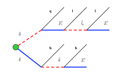
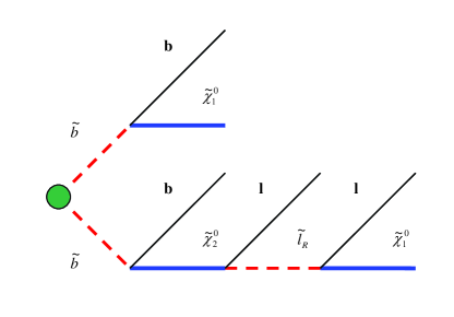
Figure 2: Examples of SUSY background processes: neutralinos appear in wrong vertices (left); gluino is missing (right).

For the second type of background (Figure 2) only one b-quark appears in a wrong vertex which effectively leads to smearing in momentum of the corresponding b-jet. As a result, for reasonably small smearing these processes, even though they are background, can give quite correct mass peak positions upon reconstruction.

III. Preliminary estimate of light masses by the endpoint method

The endpoint method has been widely used to determine masses of SUSY particles  [5] in particular in application to a decay chain

$$\tilde{q_{L}}\to\tilde{\chi}_{2}^{0}q\to\tilde{l}_{R}l_{near}q\to\tilde{\chi}_{1}^{0}l_{far}l_{near}q$$ (3)

which is a subprocess of the cascade (1) if one considers $\tilde{q_{L}}$ instead of $\tilde{b}$. For leptons in the process (3) the following notations are used: $l_{near}$ stands for a lepton which is “nearer” to the quark while the lepton radiated by the slepton is called $l_{far}$ because it is “further” from the quark.

In the process (3) there are three detectable particles: a quark and two leptons. Four invariant mass distributions can be formed from them: $\bf m_{ll}$, $\bf m_{qll}$, $\bf m_{ql_{near}}$, $\bf m_{ql_{far}}$. The $\bf m_{ll}$ and $\bf m_{qll}$ distributions are observable, in particular, the $\bf{ll}$ edge, $\bf{qll}$ edge and $\bf{qll}$ threshold can be measured. It is impossible to observe $\bf m_{ql_{near}}$ and $\bf m_{ql_{far}}$ distributions because the $\bf l_{near}$ and $\bf l_{far}$ assignment is ambiguous, however these invariant masses can be combined to give $\bf{ql}$ low and $\bf{ql}$ high edges which are observable.

Endpoint extraction

To extract endpoints from these distributions a fit was performed. The $\bf{ll}$ distribution was fitted in a standard way by a triangle form convoluted with a Gaussian. Usually the four remaining distributions are fitted near the edges by straight lines, but for 80k data samples this approach does not work, due to low statistics. Instead predefined functions covering a wider range of the distributions (0 - 1 TeV) have been used to get the endpoints. The $\bf{qll}$, $\bf{ql}$ low and $\bf{ql}$ high distributions were fitted by a parabola and a straight line in the range 0-1 TeV. The $\bf{qll}$ threshold distribution was fitted by an exponential function and a straight line in the range 0-1 TeV.

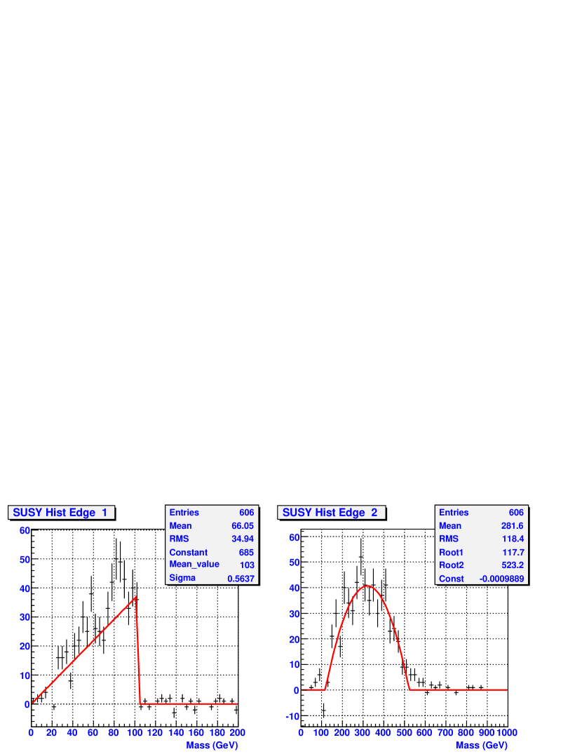
Figure 3: Invariant mass distributions for Set 1 at the SU3 point: $\bf{ll}$ edge (left), $\bf{qll}$ edge (right)

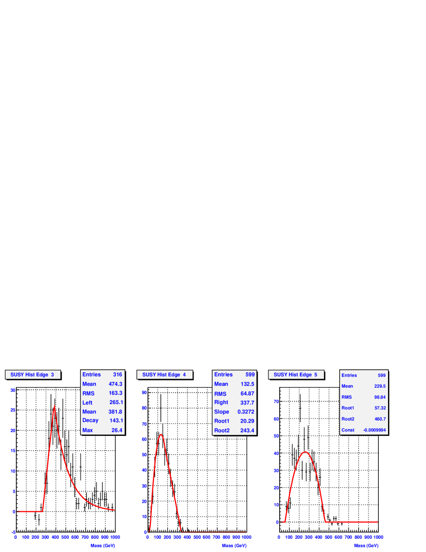
Figure 4: Invariant mass distributions for Set 1 at the SU3 point: $\bf{qll}$ threshold (left), $\bf{ql}~{}$low edge (middle) and $\bf{ql}~{}$high edge (right)

Figures (3) and (4) show five invariant mass distributions for Set 1 of 80k events at the SU3 point after applied the kinematic cuts and OSOF subtraction. For Set 1 the endpoints and reconstruction errors found from fitting of the edges are $\{$103$\pm$2, 523$\pm$6, 265$\pm$4, 338$\pm$6, 461$\pm$5$\}$ to be compared with heoretical endpoints $\{$103.1, 535.2, 263.8, 340.7, 456.0$\}$ for the SU3 point.

Mass region search

Table (4) gives the kinematic endpoints in dependence on SUSY particle masses [8],[9]. The different cases listed for $\bf{qll}$ and $\bf{ql}$ distributions are distinguished by mass ratios of sparticles.

Edge	Kinematic endpoints
$\bf ll$	$(\tilde{\xi}-\tilde{l})(\tilde{l}-\tilde{\chi})/\tilde{l}$
$\bf qll~{}threshold$	$[(\tilde{q}+\tilde{\xi})(\tilde{\xi}-\tilde{l})(\tilde{l}-\tilde{\chi})+2\tilde{l}(\tilde{q}-\tilde{\xi})(\tilde{\xi}-\tilde{\chi})-(\tilde{q}-\tilde{\xi})\sqrt{(\tilde{\xi}+\tilde{l})^{2}(\tilde{l}+\tilde{\chi})^{2}-16\tilde{\xi}\tilde{\chi}\tilde{l}^{2}}~{}]/(4\tilde{l}\tilde{\xi})$
$\bf{qll}$
$case~{}(1)$	$(\tilde{q}-\tilde{\xi})(\tilde{\xi}-\tilde{\chi})/\tilde{\xi}~{},~{}~{}~{}~{}~{}~{}~{}~{}~{}~{}~{}~{}~{}\tilde{q}/\tilde{\xi}>\tilde{\xi}/\tilde{\chi}$
$case~{}(2)$	$(\tilde{q}\tilde{l}-\tilde{\xi}\tilde{\chi})(\tilde{\xi}-\tilde{l})/(\tilde{\xi}\tilde{l})~{},~{}~{}~{}~{}~{}~{}~{}~{}\tilde{\xi}/\tilde{l}>(\tilde{l}/\tilde{\chi})(\tilde{q}/\tilde{\xi})$
$case~{}(3)$	$(\tilde{q}-\tilde{l})(\tilde{l}-\tilde{\chi})/\tilde{l}~{},~{}~{}~{}~{}~{}~{}~{}~{}~{}~{}~{}~{}~{}~{}~{}\tilde{l}/\tilde{\chi}>\tilde{q}/\tilde{l}$
$case~{}(4)$	$(\sqrt{\tilde{q}}-\sqrt{\tilde{\chi}})^{2}~{},~{}~{}~{}~{}~{}~{}~{}~{}~{}~{}~{}~{}~{}~{}~{}~{}~{}~{}~{}otherwise$
$\bf{ql}$  low,  $\bf{ql}$  high
$case~{}(1)$	$(m_{ql_{near}}^{max})^{2}~{},~{}(m_{ql_{far}}^{max})^{2}~{},~{}~{}~{}~{}~{}~{}~{}2\tilde{l}/\tilde{\chi}>\tilde{\xi}/\tilde{\chi}+1$
$case~{}(2)$	$(m_{ql_{bound}}^{max})^{2}~{},~{}(m_{ql_{far}}^{max})^{2}~{},~{}~{}~{}~{}~{}~{}~{}~{}~{}\tilde{\xi}/\tilde{\chi}+1>2\tilde{l}/\tilde{\chi}>2\sqrt{\tilde{\xi}/\tilde{\chi}}$
$case~{}(3)$	$(m_{ql_{bound}}^{max})^{2}~{},~{}(m_{ql_{near}}^{max})^{2}~{},~{}~{}~{}~{}~{}2\sqrt{\tilde{\xi}/\tilde{\chi}}>2\tilde{l}/\tilde{\chi}$

Table 4: The kinematic endpoints for the process (3). The following notations are used for masses $\tilde{\chi}=m_{\tilde{\chi}_{1}^{0}}^{2}$ , $\tilde{l}=m_{\tilde{l}_{R}}^{2}$ , $\tilde{\xi}=m_{\tilde{\chi}_{2}^{0}}^{2}$ , $\tilde{q}=m_{\tilde{q}}^{2}$ and endpoints $(m_{ql_{near}}^{max})^{2}=(\tilde{q}-\tilde{\xi})(\tilde{\xi}-\tilde{l})/\tilde{\xi}$, $(m_{ql_{far}}^{max})^{2}=(\tilde{q}-\tilde{\xi})(\tilde{l}-\tilde{\chi})/\tilde{l}$, $(m_{ql_{bound}}^{max})^{2}=(\tilde{q}-\tilde{\xi})(\tilde{l}-\tilde{\chi})/(2\tilde{l}-\tilde{\chi}).$ For $\bf{qll}$ and $\bf{ql}$ edges endpoints are given by different expressions in dependence on mass ratios.

While the $\bf{ll}$ edge and $\bf{qll}$ thresholds are given by unique expressions, the other endpoints have different formulas for different mass ratios which are not known $a~{}priori$: there are four expressions for the $\bf{qll}$ edge and three expressions for $\bf{ql}$ low and $\bf{ql}$ high edges. Each overall combination corresponds to a unique mass region in SUSY particle mass space $m_{\tilde{q_{L}}}$, $m_{\tilde{\chi}_{2}^{0}}$, $m_{\tilde{l}_{R}}$, $m_{\tilde{\chi}_{1}^{0}}$. These mass regions defined by mass ratios from Table (4) are labeled by R(i,j), where i=1,2,3,4 and j=1,2,3 denote the corresponding mass ratios for $\bf{qll}$ and $\bf{ql}$ endpoints, respectively. According to the analysis performed in [9] only nine of these 12 $(4\times 3)$ combinations are physical, the regions R(2,1), R(2,2), and R(3,3) are not possible. Additionally, the regions R(2,3), R(3,1), and R(3,2) are degenerate: the invariant mass distributions are not linearly independent, because the $\bf{qll}$ edge is the function of the $\bf{ll}$ and $\bf{ql}$ high edges.

A procedure was developed to determine from the data sample the SUSY particle mass-space region. Once the SUSY mass region is defined, the endpoint expression is determined in a unique way from Table 4. Expressions for endpoints are inverted to get masses in terms of endpoints. Four endpoints are required to invert the formulas because there are four unknown masses in the process (3). For formula inversion we always use the $\bf{ll}$ distribution because it gives the endpoint with relatively high precision and we take any three endpoints of the remaining four. For example, one can extract four sparticle masses by considering either $\bf{ll,~{}qll}$, $\bf{ql}$ low, $\bf{ql}$ high combination of endpoints or $\bf{ll,~{}qll}$, $\bf{ql}$ low, $\bf{qll}$ threshold combination and so on. Thus for each region R(1,1), R(1,2), R(1,3), R(4,1), R(4,2), R(4,3) we get four different sets of mass formulas. For degenerate regions R(2,3), R(3,1), R(3,2) we get only two sets of mass formulas because there are only four independent endpoints. Note that inverse formulas are very sensitive to the endpoint determination precision because some formulas contain singularities in the range of 30 GeV around actual endpoints. The use of the full shapes of the signal as it was proposed in [18],[19] could lead to an improvement in endpoint extraction.

The SUSY mass region is accepted if for all sets of inverse formulas the hierarchy condition $m_{\tilde{q_{L}}}~{}>~{}m_{\tilde{\chi}_{2}^{0}}~{}>~{}m_{\tilde{l}_{R}}~{}>~{}m_{\tilde{\chi}_{1}^{0}}~{}>~{}20~{}GeV$ is satisfied and found masses correspond to the mass ratios of Table (4). Variations of low mass bound on the lightest neutralino mass in the range 20-50 GeV does not affect the results. Note that the limit from accelerator experiments on $m_{\tilde{\chi}_{1}^{0}}$ is $46~{}GeV$ [20].

For all five SU3 data sets the R(1,3) region in mass space was found, which is the true region for the SU3 point. Note that the mass region search is sensitive to fluctuations in invariant mass distributions. An increase in integrated luminosity should lead to more precise reconstruction of light SUSY particle masses.

Preliminary estimation of light SUSY particle masses

Once endpoints are found and mass regions are defined, sparticle masses can be determined by a minimization of $\chi^{2}$. Parameters $\vec{m}$ of a $\chi^{2}$ fit are the four sparticle masses $m_{\tilde{q_{L}}}$, $m_{\tilde{\chi}_{2}^{0}}$, $m_{\tilde{l}_{R}}$, $m_{\tilde{\chi}_{1}^{0}}$. The $\chi^{2}$, as a function of the free parameters $\vec{m}$, is then given by

$$\chi^{2}(\vec{m})=\sum_{i=1}^{5}\frac{(Q_{i}^{obs}-Q_{i}(\vec{m}))^{2}}{\sigma_{i}^{2}}$$ (4)

Expression $Q_{i}(\vec{m})$ is the endpoint as a function of sparticle masses for the corresponding SUSY mass region as given in Table (4). $Q_{i}^{obs}$ are the observable endpoints and their errors $\sigma_{i}$ determined in the above procedure.

The results of the fit for preliminary mass estimates and their errors based on found endpoints, edge reconstruction errors and mass regions are summarized in Table (5).

Point	Particle	Set 1	Set 2	Set 3	Set 4	Set 5
SU3	$\tilde{\chi}_{2}^{0}$	201$\pm$33	245$\pm$25	206$\pm$36	252$\pm$46	199$\pm$34
	$\tilde{l}_{R}$	130$\pm$33	179$\pm$27	133$\pm$34	184$\pm$47	128$\pm$27
	$\tilde{\chi}_{1}^{0}$	96$\pm$29	140$\pm$26	104$\pm$30	147$\pm$46	93$\pm$28

Table 5: Light masses preliminary determined from fitting of edges for the SU3 point.

IV. Event filter

An event filter is required before the final fit to determine the heavy SUSY particle ($\tilde{g}$, $\tilde{b}$) mass range and suppress background. It is very important to reduce combinatorial background because at the final stage of the reconstruction procedure all possible five event combinations are considered. The combinatorial background is defined as five-event combinations that include at least one background event. The number of five-event combinations including only signal events is given by $N_{s}=n_{s}!/(5!(n_{s}-5)!)$ where $n_{s}$ is the number of signal events in a data sample. The total number of five-event combinations including backgrounds is given by $N_{tot}=(n_{s}+n_{b})!/(5!(n_{s}+n_{b}-5)!)$ where $n_{b}$ is the number of background events in a data sample. The contribution of combinatorial background with respect to all possible five signal events combinations $(N_{tot}-N_{s})/N_{s}$ in the case of high $n_{s}$ can be approximated by $((n_{s}+n_{b})/n_{s})^{5}$ which is of about 240 for the SU3 point, as follows from Table 3. At the event filter stage we can reduce the 5-dimensional mass space for each event to a 2-dimensional one, supposing that three light SUSY particle masses ($\tilde{\chi}_{2}^{0}$, $\tilde{l}_{R}$, $\tilde{\chi}_{1}^{0}$) are fixed and taken as the preliminary masses found by the endpoint method in the previous chapter.

The event filter procedure is based on an approximate likelihood function with the mass relation constraint for each event

$$L(m_{\tilde{g}},m_{\tilde{b}})=\prod_{i=1}^{4}~{}exp\left[-\frac{(p_{i}^{event}-p_{i}^{meas})^{2}}{2\sigma_{i}^{2}}\right]$$ (5)

where index i runs over observed particles (two b-quarks and two leptons) and labels the measured absolute momenta $p_{i}^{meas}$, the uncertainties $\sigma_{i}$ in their measurement, and the event true absolute momenta $p_{i}^{event}$. The approximate likelihood function (5) takes into account only uncertainties in lepton and b-jet energy measurements. Note that positions of each of two b-jets and of each of two leptons in the decay chain (1) are unknown. It is quite simple to resolve the b-jets assignment because usually (about $96\%$ of the time) the b-jet with higher $p_{T}$ originates from $\tilde{b}$-quark decay, since for SU3 point at rest system $p_{Tb_{1}}=(m_{\tilde{b}}^{2}-m_{\tilde{\chi}_{2}^{0}}^{2})/2m_{\tilde{b}}\gg p_{Tb_{2}}=(m_{\tilde{g}}^{2}-m_{\tilde{b}}^{2})/2m_{\tilde{g}}$. Therefore for each event we assume that the b-jet with higher $p_{T}$ originates from $\tilde{b}$-quark decay. Leptons with higher $p_{T}$ are produced in both vertices with comparable probabilities. In this work for simplicity it is assumed that leptons with higher $p_{T}$ originate from $\tilde{l}_{R}$ decay. We use the following parametrization for $\sigma_{i}$ in equation (5): for b-jets    $\sigma/E=0.5/\sqrt{E(GeV)}~{}\oplus~{}0.03$ and leptons $\sigma/E=0.12/\sqrt{E(GeV)}~{}\oplus~{}0.005.$

To find a maximum of the likelihood function (5) with the constraint (2) is the same as to search for a minimum of $\chi^{2}=-2\cdot\rm{logL}~{}$ function:

$$\chi^{2}(m_{\tilde{g}},m_{\tilde{b}})=\sum_{i=1}^{4}\frac{(p_{i}^{event}-p_{i}^{meas})^{2}}{\sigma_{i}^{2}}+\lambda f(\vec{m},\vec{p})~{}$$ (6)

In Eq.(6) the mass relation constraint $f(\vec{m},\vec{p})$ (2) is taking into account by the Lagrange multiplier $\lambda$. We construct an event likelihood distribution calculating minimum of the $\chi^{2}$ function (6) for each of 10⁵ randomly defined points in the ($\tilde{g}$, $\tilde{b}$) mass plane, assuming that they are distributed uniformly in the range $0.4-1.4TeV$ and $0.3-1.3TeV$, respectively. This effectively corresponds to a two dimensional grid with spacing of $3GeV\times 3GeV$. We add points ($m_{\tilde{g}}$, $m_{\tilde{b}}$) with a weight equal to $(\chi_{cut}^{2}-\chi^{2})/2$ to an event likelihood distribution histogram if the minimization procedure of the function (6) converges, $\chi^{2}(m_{\tilde{g}},m_{\tilde{b}})<\chi_{cut}^{2}=10$ and $f<10^{-4}GeV^{2}$. The minimization iteration procedure is considered to have converged if the relative difference in $\chi^{2}_{event}$ for two consecutive iteration steps is less than $0.5\%$ and the total number of iteration steps does not exceed 20. For signal events the event likelihood distribution has a maximum in the region of the ($\tilde{g}$, $\tilde{b}$) mass plane correlated with the true masses of $\tilde{g}$ and $\tilde{b}$. Thus signal events should give a peak in the region of true masses. For background events there is no strong correlation of maximum likelihood distribution with true ($\tilde{g}$, $\tilde{b}$) masses. We define the combined event likelihood function as

$$\rm{log}~{}L_{comb}(m_{\tilde{g}},m_{\tilde{b}})=\sum_{events}{\rm{log}~{}L(m_{\tilde{g}},m_{\tilde{b}})}$$ (7)

where the sum includes all events in the data sample.

Figure (5) shows two projection histograms of combined event likelihood distribution versus gluino mass $m_{\tilde{g}}$ and versus difference of gluino and sbottom masses ($m_{\tilde{g}}-m_{\tilde{b}}$ for Set 1. The variables ($m_{\tilde{g}}$, $m_{\tilde{g}}-m_{\tilde{b}}$) are used because an event likelihood distribution is more sensitive to these variables. Preliminary estimates for heavy sparticle masses and mass errors (the mean values and standard deviations) obtained by fitting of these histograms by a Gaussian near the peak region are given in Table 6 for all five sets.

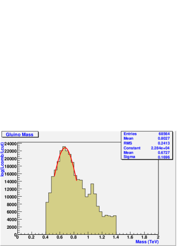
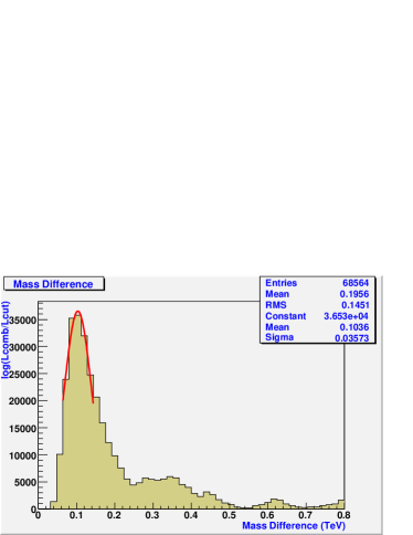
Figure 5: Combined event likelihood projection histograms for Set 1 at the SU3 point.

Particle	Set 1	Set 2	Set 3	Set 4	Set 5
$\tilde{g}$	673$\pm$170	720$\pm$124	683$\pm$158	729$\pm$211	649$\pm$110
$\tilde{b}$	569$\pm$174	615$\pm$135	577$\pm$162	621$\pm$214	536$\pm$116

Table 6: Preliminary heavy SUSY particle masses and mass errors estimated by event filter.

To suppress the background the previous procedure constructing an event likelihood distribution is repeated, but in the narrow range in $m_{\tilde{g}}$ and $m_{\tilde{b}}$: $m_{\tilde{g}}\pm\sigma$, $m_{\tilde{b}}\pm\sigma$ from Table 6, assuming the uniform distributions. Requiring convergence and applying $\chi^{2}$ and the constraint f cuts as above results in a likelihood distribution histogram that has high efficiency for a signal event and low efficiency for background events. Typically for a signal event the likelihood distribution histogram has of a few thousand entries (recall that the procedure is repeated $10^{5}$ times). In order to reject background and not suppress signal, an entry threshold of 300 is chosen. Thus if the event likelihood distribution histogram has greater than 300 entries the event is considered a signal candidate and it is retained for the consequent analysis.

After the application of the event filter the ratio of background events to signal events is reduced approximately by a factor 2 as can be seen from Table 7 .

Set	Total	Signal	SUSY	Ratio
	Number	Events	Backg.
1	154/83	47/39	107/44	3.3/2.1
2	131/83	48/42	83/41	2.7/2.0
3	148/76	44/35	104/41	3.4/2.2
4	157/110	50/45	107/65	3.1/2.4
5	141/89	55/45	86/44	2.6/2.0
1-5	731/441	244/206	487/235	3.0/2.1

Table 7: The number of signal and background events before/after an application of event filter to 80k SUSY events. The last row shows the sum over all five sets.

Contribution of the combinatorial background which is given approximately by ((Signal+Background)/Signal)⁵ is therefore significantly suppressed. The suppression factor for the SU3 point varies from 3 to 9.

V. Combinatorial method for final mass reconstruction

A combinatorial procedure is used for the final SUSY particle mass reconstruction. It is applied only to the events that pass the event filter. In order to explain this point let’s neglect for a moment uncertainties in detected particle momenta and the widths of the Breit-Wigner distribution. For a single event the mass relation constraint represents a four dimensional surface in five-mass parameter space. Therefore, for two events the intersection of two four dimensional surfaces is a three dimensional surface and correspondingly for three events one gets a two dimensional surface of intersection, for four events the surface is one dimensional and at last for five events the intersection is just a point or a few points in five dimensional mass space corresponding to SUSY particle masses. Thus in an ideal case five events would be enough [12] to reconstruct masses of SUSY particles. Uncertainties in detected particle momenta and Breit-Wigner distribution lead to smearing in the position of this point. There is a trade-off between the number of events in a combination and combinatorial background: more events restrict the number of degrees of freedom and better define SUSY masses, but combinatorial background increases. Therefore, at the final stage of mass reconstruction when the physical background has already been reduced, we will consider all possible five event combinations from the event sample. Recall that in reality due to the Breit-Wigner distribution the masses of the gluino and bottom squark vary from event to event. A method described below takes into account that SUSY particle masses can vary from event to event.

SUSY particle masses are reconstructed by a search for a maximum of a combined likelihood function constructed for each possible combination of five events in the data sample. For sparticle masses ($\vec{m}$) the combined likelihood function for the combination is defined as the product of the maximum likelihood functions for individual events. To find a maximum of the combined likelihood function for the combination is the same as to search for a minimum of the function

$$\chi^{2}_{comb}(\vec{m})=\sum_{i=1}^{5}{\rm{MIN}(\chi^{2}_{~{}event})_{i}}$$ (8)

where $\chi^{2}_{comb}=-2\cdot\rm{logL_{comb}}$. In Eq.(8) $\rm{MIN}(\chi^{2}_{event})_{i}$ is a result of searching for a minimum of the $\chi^{2}_{event}$ function (9) for an individual event for given $\vec{m}$ with the mass relation and ${\bf ll}$ edge constraints. For each of the five events in the five event combination the $\rm{MIN}(\chi^{2}_{event})$ is fitted with 9 parameters (four particle momenta and five SUSY masses) starting with $\vec{p}^{~{}event}=\vec{p}^{~{}meas}$ and $\vec{m}^{event}=\vec{m}$. The minimization iteration procedure is converged if a relative difference in $\chi^{2}_{event}$ for two consecutive iteration steps is less than $0.5\%$ and the total number of iteration steps does not exceed 20.

The $\chi^{2}$ function for an event is defined by

$$\chi^{2}_{event}=\sum_{i=1}^{4}\frac{(p_{i}^{event}-p_{i}^{meas})^{2}}{\sigma_{i}^{2}}+\sum_{n=1}^{5}\frac{(m_{n}^{event}-m_{n})^{2}}{\sigma_{n}^{2}}+\lambda_{1}f+\lambda_{2}f^{ll}~{}.$$ (9)

where the first term takes into account deviations of measured momenta of b-jets and leptons from the true ones. The second term takes into account that sparticles are varied from event to event and approximated by a Gaussian of width $\sigma_{n}$ instead a Breit-Wigner distribution. In Eq.(9) the mass relation and $\bf{ll}$ edge constraints are taking into account by Lagrange multiplier $\lambda_{1},\lambda_{2}$. Standard deviations corresponding to the mass term are taking to be 15 GeV for the gluino, 5 GeV for bottom squark and 1 GeV for light masses. The first two numbers are comparable with theoretical widths for heavy SUSY particles. The last number takes into account the fact that light SUSY particles are quite narrow or stable. We note that the results of the mass reconstruction are not strongly sensitive to actual values of sparticle widths.

To get a starting point for the minimization of $\chi^{2}_{comb}$ for each five-event combination we calculate $\chi^{2}_{comb}$ for 3000 $\vec{m}$ values produced with a simple Monte Carlo. The set of the mass $\vec{m}$ with the smallest $\chi^{2}_{comb}$ is used as the starting point. It is assumed that heavy masses are distributed uniformly in the following range: mean value $\pm~{}2\sigma$, where the mean values and standard deviations are given in Table 6 as the results of event filter application. For the three light masses the Gaussian distribution is assumed with mean values and standard deviations found by the endpoint technique as given in Table 5. The starting point is used by MINUIT code with the Simplex algorithm to search for the minimum of $\chi^{2}_{comb}$ with five parameters $\vec{m}$. The five-event combination is added to reconstruction mass histograms if the MINUIT minimization procedure converges, $~{}\chi^{2}_{comb}<\chi_{cut}^{2}=10$ and the sum of the mass relation and $\bf{ll}$ edge constraint functions for five events is less than 1 $GeV^{2}$. The CPU time required for the final minimization of the five-event combination is about 2 second for a 3GHz processor. For a set of 100 events the required time for combinatorial mass reconstruction would be about 7 years. In order to reduce the computational time, we divide a sample of 80k SUSY events into four subsets of 20k. Forming combinations only from events within each 20k subset greatly reduces combinatorics. Because the total set is subdivided in four subsets the procedure is carried on for each subset and reconstruction mass histograms are merged.

Reconstructed SUSY particle mass distributions and results of fitting these distributions by a Gaussian are presented in Figures (6 and 7) for Set 1 at the SU3 point with integrated luminosity 4.2 $\rm fb^{-1}$. As can be seen in these Figures, the reconstructed mass distributions are well described by a Gaussian. The mean values of the Gaussian fit are considered as the reconstructed sparticle masses. As can been seen these masses are close to the theoretical masses. It is assumed that mass reconstruction errors are given by the Gaussian fit standard deviations. For the light sparticles the final procedure improves mass reconstruction errors by a factor of 2 but the masses are changed only slightly in comparison with the preliminary estimate.

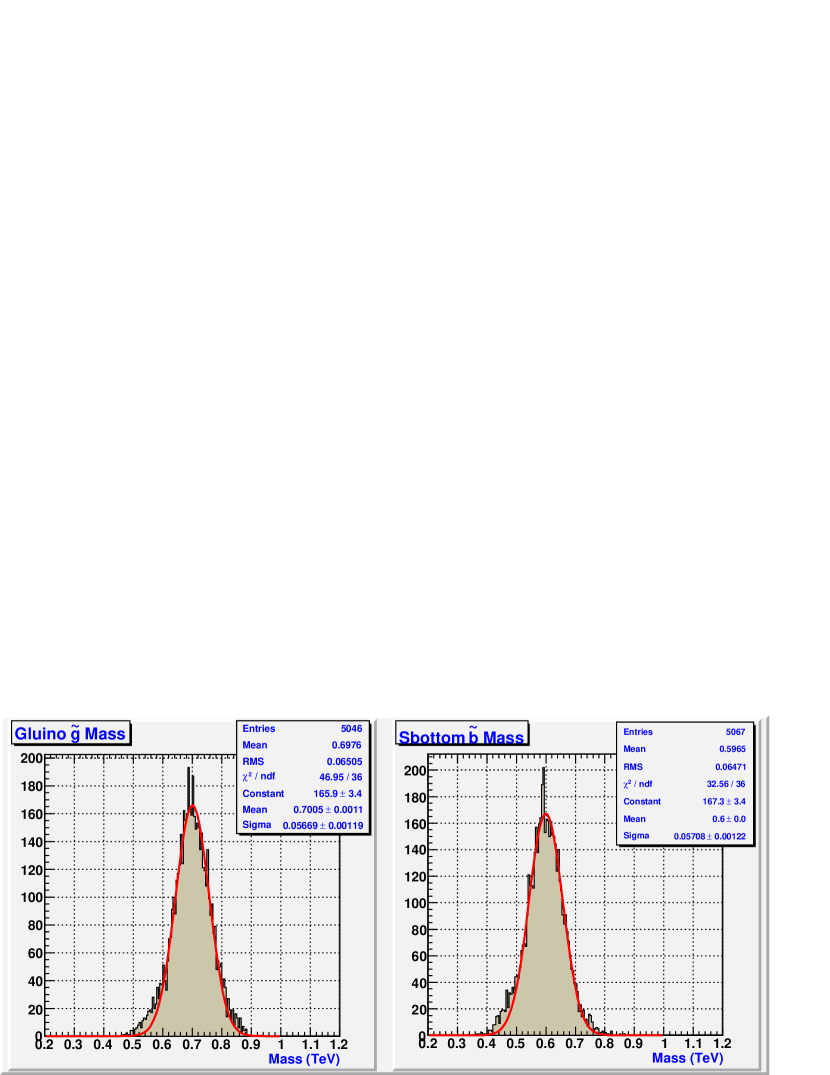
Figure 6: Reconstructed heavy SUSY particle mass distributions for Set 1, including background with integrated luminosity 4.2 $\rm fb^{-1}$: gluino $\tilde{g}$ (left), sbottom $\tilde{b}$ (right). The line is a result of Gaussian fit.

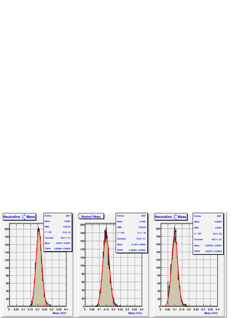
Figure 7: Reconstructed light SUSY particle mass distributions for Set 1, including background with integrated luminosity 4.2 $\rm fb^{-1}$: neutralino $\tilde{\chi}_{2}^{0}$ (left), slepton $\tilde{l}_{R}$ (middle), neutralino $\tilde{\chi}_{1}^{0}$ (right). The line is a result of Gaussian fit.

Final results of this mass reconstruction approach are presented for five data sample sets of 80k events each in Table 8.

Set	$m_{\tilde{g}}$	$m_{\tilde{b}}$	$m_{\tilde{\chi}_{2}^{0}}$	$m_{\tilde{l}_{R}}$	$m_{\tilde{\chi}_{1}^{0}}$
1	701$\pm$57	600$\pm$57	208$\pm$21	148$\pm$23	98$\pm$22
2	712$\pm$55	608$\pm$53	254$\pm$21	183$\pm$23	143$\pm$20
3	664$\pm$78	564$\pm$80	219$\pm$24	149$\pm$24	109$\pm$23
4	767$\pm$62	649$\pm$65	258$\pm$35	193$\pm$35	148$\pm$34
5	655$\pm$45	545$\pm$47	208$\pm$21	138$\pm$22	96$\pm$20

Table 8: Reconstructed SUSY particle masses and reconstruction errors for five data sample sets of 80k events each.

In order to illustrate a spread in reconstructed masses the results of Table 8 are also shown in a form of ideograms [21] in Figures (8 and 9) for the five data sample sets. Each reconstructed mass in an ideogram is represented by a Gaussian with a central value $m_{i}$, error $\sigma_{i}$ and area proportional to 1/$\sigma_{i}$. The solid curve is a sum of these Gaussians.

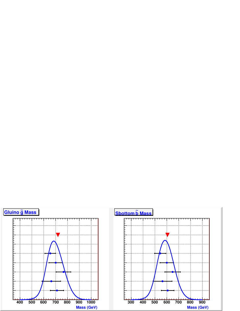
Figure 8: Ideograms of reconstructed heavy SUSY particle masses, including background for five data sample sets with integrated luminosity 4.2 $\rm fb^{-1}$: gluino $\tilde{g}$ (left), sbottom $\tilde{b}$ (right). The triangle marker gives the position of theoretical mass. Points with error bars correspond to five data sample sets.

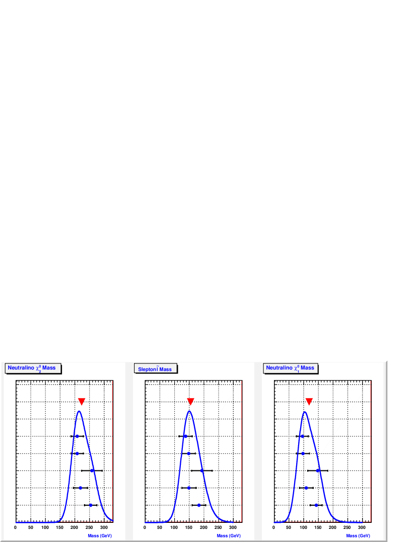
Figure 9: Ideogram of reconstructed light SUSY particle mass distributions, including background for five data sample sets with integrated luminosity 4.2 $\rm fb^{-1}$: neutralino $\tilde{\chi}_{2}^{0}$ (left), slepton $\tilde{l}_{R}$ (middle), neutralino $\tilde{\chi}_{1}^{0}$ (right). Triangle marker gives the position of theoretical mass. Points with error bars correspond to five data sample sets.

The Gaussian form of ideograms and relatively small shift of peak positions with respect to theoretical masses demonstrate the self-consistency of the mass reconstruction approach.

IX. Conclusion

We have developed an approach that allows extracting all SUSY particle masses for long cascades at the LHC with an integrated luminosity of a few $\rm fb^{-1}$. This luminosity can be reached at the early stage of the LHC in comparison with a projected integrated luminosity of $300~{}\rm fb^{-1}$ in five years. This approach is based on a consecutive use of the endpoint method, an event filter and a combinatorial mass reconstruction method.

The endpoint method allows preliminary estimate of light SUSY particle ($\tilde{\chi}_{2}^{0},\tilde{l}_{R},\tilde{\chi}_{1}^{0}$) masses in a model-independent way.

The light sparticle masses are used to construct the maximum likelihood distribution in the two heaviest-sparticle mass-plane for each individual event taking into account the mass relation equation constraint. The event filter combining the maximum likelihood distributions for all events in the data sample allows a determination of the range of heavy sparticle masses and significant suppression of background. This is a new technique for background suppression. Note that in this work we did not use $\tau$ tagging for background suppression. The application of $\tau$ tagging could provide an additional suppression of combinatorial SUSY background by approximately a factor of 2.

Finally, SUSY particle $(\tilde{g},\tilde{b},\tilde{\chi}_{2}^{0},\tilde{l}_{R},\tilde{\chi}_{1}^{0})$ masses are extracted by a search for a maximum of a combined likelihood function constructed for each possible combination of five events in the data sample satisfying the filter. Mass peaks for five sparticles are clearly reconstructed because the remaining background does not exhibit peaks corresponding to the signal region. With more events the same technique could be used to reconstruct, for example, masses of the $\tilde{\tau}_{1}$ and $\tilde{t}_{1}$ in the following cascade decays: $\tilde{g}\to\tilde{b}\to\tilde{\chi}_{2}^{0}\to\tilde{\tau}_{1}\to\tilde{\chi}_{1}^{0}$ and $\tilde{g}\to\tilde{t_{1}}\to\tilde{\chi}_{2}^{0}\to\tilde{l}_{R}\to\tilde{\chi}_{1}^{0}$.

SUSY data sample sets for this work were generated for the benchmark SU3 point of mSUGRA scenario. A detector response was parametrized by the AcerDET detector simulator. The stability and precision of the approach was demonstrated by considering five different 80k event data sets for each model point. Masses were reconstructed with a precision of about $10\%$ for heavy sparticles and $10\%,15\%$ and $20\%$ for light $\tilde{\chi}_{2}^{0},\tilde{l}_{R}$ and $\tilde{\chi}_{1}^{0}$ sparticles, respectively. The precision of mass reconstruction with this technique should be improved with an increase in integrated luminosity.

We also applied the cascade mass reconstruction approach to SPS1a model point of mSUGRA parameter space and masses were reconstructed with the same precision as for the SU3 point.

The approach developed in this paper can be used for the ATLAS and CMS detectors at the LHC; or at the future ILC.

Appendix A. Mass relation equation

The mass relation method [12] is based on a solution of a system of kinematic equations obtained for each vertex of decay cascade. For the chain (1) the system of kinematic equations is given by four equations corresponding to four vertices

$m_{\tilde{l}_{R}}^{2}=(p_{\tilde{\chi}_{1}^{0}}+k_{l_{1}})^{2}$

$m_{\tilde{\chi}_{2}^{0}}^{2}=(p_{\tilde{\chi}_{1}^{0}}+k_{l_{1}}+k_{l_{2}})^{2}$

$m_{\tilde{b}}^{2}=(p_{\tilde{\chi}_{1}^{0}}+k_{l_{1}}+k_{l_{2}}+p_{b_{1}})^{2}$

$m_{\tilde{g}}^{2}=(p_{\tilde{\chi}_{1}^{0}}+k_{l_{1}}+k_{l_{2}}+p_{b_{1}}+p_{b_{2}})^{2}$

This system of four equations can be easily modified to a linear system defining four component of lightest neutralino four-momentum

$$Sp_{\tilde{\chi}_{1}^{0}}=Q,$$ (10)

where matrix S is given by

$$\begin{pmatrix}k_{l_{1}}^{0}&-k_{l_{1}}^{1}&-k_{l_{1}}^{2}&-k_{l_{1}}^{3}\\ k_{l_{2}}^{0}&-k_{l_{2}}^{1}&-k_{l_{2}}^{2}&-k_{l_{2}}^{3}\\ p_{b_{1}}^{0}&-p_{b_{1}}^{1}&-p_{b_{1}}^{2}&-p_{b_{1}}^{3}\\ p_{b_{2}}^{0}&-p_{b_{2}}^{1}&-p_{b_{2}}^{2}&-p_{b_{2}}^{3}\par\end{pmatrix}$$

$p_{\tilde{\chi}_{1}^{0}}$ is the column vector of lightest neutralino four-momentum

$$\begin{pmatrix}p_{\tilde{\chi}_{1}^{0}}^{0}\\ p_{\tilde{\chi}_{1}^{0}}^{1}\\ p_{\tilde{\chi}_{1}^{0}}^{2}\\ p_{\tilde{\chi}_{1}^{0}}^{3}\par\end{pmatrix}$$

Q is the column vector of coefficients

$$\begin{pmatrix}b\\ c-k_{l_{1}}\cdot k_{l_{2}}\\ d-p_{b_{1}}\cdot(k_{l_{1}}+k_{l_{2}})\\ e-p_{b_{2}}\cdot(k_{l_{1}}+k_{l_{2}}+p_{b_{1}})\par\end{pmatrix}$$

where

$b=0.5*(m_{\tilde{l}_{R}}^{2}-m_{\tilde{\chi}_{1}^{0}}^{2})$

$c=0.5*(m_{\tilde{\chi}_{2}^{0}}^{2}-m_{\tilde{l}_{R}}^{2})$

$d=0.5*(m_{\tilde{b}}^{2}-m_{\tilde{\chi}_{2}^{0}}^{2})$

$e=0.5*(m_{\tilde{g}}^{2}-m_{\tilde{b}}^{2})$

Lepton and quark masses are neglected in these equations.

The solutions of linear equation (10) is given by standard formulas

$$p_{\tilde{\chi}_{1}^{0}}^{j}=detS_{j}/detS$$ (11)

where the submatrix $S_{j}$ is formed by substituting elements of vector Q instead of $j^{th}$ column of matrix S.

By using on-shell mass condition $m_{\tilde{\chi}_{1}^{0}}^{2}=p_{\tilde{\chi}_{1}^{0}}^{2}$ for the lightest neutralino with momentum components from (11) one gets the following equation

$$f=(detS_{0}/detS)^{2}-\sum_{j=1}^{j=3}(detS_{j}/detS)^{2}-m_{\tilde{\chi}_{1}^{0}}^{2}=0.$$ (12)

Equation (12) is the basic equation of mass relation method and it gives the relation between masses of five SUSY particles. Each event is represented as a curve in five dimensional mass space. Coefficients of this equation are functions of the four-momenta of detected particles where b quarks are measured as jets in the detector.

References

-
[1]
Y.Gelfand and E.Likhtman, JETP Lett.(1971)323;
P.Ramond, Phys.Rev.(1971)2415;
A.Neveu and J.H.Schwartz, Nucl.Phys.(1971)86;
J.L.Jervais and B.Sakita, Nucl.Phys.(1971)632;
D.Volkov and V.Akulov, Phys.Lett.(1973)109;
J.Wess and B.Zumino, Nucl.Phys.(1974)39;
P.Fayet, Phys.Lett.(1976)159;
P.Fayet and S.Ferrara, Phys.Rep.(1977)249;
H.P.Nilles, Phys.Rep.(1984)1;
H.E.Haber and G.L.Kane, Phys.Rep.(1985)75. -
[2]
S.Weinberg, Phys.Rev.(1976)974;Phys.Rev.(1979)1277;
L.Susskind, Phys.Rev.(1979)2619;
G.’t Hooft, in Recent developments in gauge theories, Proceedings of the NATO Advance Summer Institute, Cargese 1979, ed. G.’t Hooft et al. (Plenum, New York 1980). - [3] ATLAS Collaboration, ATLAS detector and physics performance. Technical design report, CERN/LHCC 99-14/15(1999).
- [4] S.Abdullin et al. [CMS Collaboration], J.Phys.(2002)469.
-
[5]
I.Hinchliffe et al.,Phys.Rev.(1997)5520;
I.Hinchliffe and F.E.Paige, Phys.Rev.(2000)095011;
H.Bachacou, I.Hinchliffe and F.E.Paige, Phys.Rev.(2000)015009. -
[6]
B.C.Allanach, C.G.Lester, M.A.Parker and B.R.Webber, JHEP
(2000)004. - [7] B.K.Gjelsten et al., ATLAS internal note ATL-PHYS-2004-007(2004), published in G.Weiglein et al. [LHC/LC Study group], arXiv:hep-ph/0410364.
- [8] B.K.Gjelsten, D.J.Miller and P.Osland, JHEP(2004)003.
- [9] B.K.Gjelsten, D.J.Miller and P.Osland, JHEP(2005)015.
- [10] C.G.Lester, M.A.Parker and M.J.White, JHEP(2006)080.
- [11] M.M.Nojiri, G.Polesello and D.R.Tovey, arXiv:hep-ph/0312317
- [12] K.Kawagoe, M.M.Nojiri and G.Polesello, Phys.Rev.(2005)035008.
- [13] C.G.Lester, arXiv:hep-ph/0402295, part X.
- [14] D.N.Spergel et al.,ApJS(2007)377.
-
[15]
L.E.Ibanez, Phys.Lett.(1982)73;
K.Inoue, A.Kakuto, H.Komatsu and S.Takeshita, Prog.Theor.Phys.
(1982)927;
A.H.Chamseddine, R.Arnowitt and P.Nath, Phys.Rev.Lett.
(1982)970;
J.R.Ellis, D.V.Nanopoulos and K.Tamvakis, Phys.Lett.(1983)123;
L.Alvarez-Gaume, J.Polchinski and M.B.Wise, Nucl.Phys.
(1983)495. - [16] G.Marchesini et al.,Comput.Phys.Commun.(1992)465; G.Corcella et al., JHEP(2001)010; S.Moretti et al., JHEP(2002)028.
- [17] E.Richter-Was, arXiv:hep-ph/0207355.
- [18] D.J.Miller, P.Osland and A.R.Raklev, JHEP(2006)034.
- [19] C.G.Lester, Phys.Lett.(2007)39.
- [20] J.Abdallah et al., Eur.Phys.J.(2003)421.
- [21] W.-M.Yao et al., J.Phys.(2006)1.