The QSO proximity effect at redshift $\langle z\rangle\simeq 2.6$ with the FLO approach

Abstract

We revisit the proximity effect produced by QSOs at redshifts $2.1-3.3$ applying the FLO approach (Saitta et al., 2007) to a sample of $\sim 6300$ Ly$\alpha$ lines fitted in 21 high resolution, high signal-to-noise spectra. This new technique allows to recover the hydrogen density field from the H i column densities of the lines in the Ly$\alpha$ forest, on the basis of simple assumptions on the physical state of the gas. To minimize the systematic uncertainties that could affect the density recovering in the QSO vicinity, we carefully determined the redshifts of the QSOs in our sample and modelled in detail their spectra to compute the corresponding ionising fluxes. The mean density field obtained from the observed spectra shows a significant over-density in the region within 4 proper Mpc from the QSO position, confirming that QSOs are hosted in high density peaks. The absolute value of $\rho/\langle\rho\rangle$ for the peak is uncertain by a factor of $\sim 3$, depending on the assumed QSO spectral slope and the minimum H i column density detectable in the spectra. We do not confirm the presence of a significant over-density extending to separations of $\sim 15$ proper Mpc from the QSO, claimed in previous works at redshifts $\langle z\rangle\simeq 2.5$ and 3.8. Our best guess for the UV background ionisation rate based on the IGM mean density recovered by FLO is $\Gamma_{\rm UVB}\simeq 10^{-12}$ s^-1. However, values of $\Gamma_{\rm UVB}\simeq 3\times 10^{-12}$ s^-1 could be viable if an inverted temperature-density relation with index $\alpha\simeq-0.5$ is adopted.

1 Introduction

The ultraviolet radiation emitted by quasars (QSOs) is considered the dominant source of ionisation of the intergalactic medium (IGM) at redshifts 2-4. Most of the absorption lines seen blue-ward of the Ly$\alpha$ emission in QSO spectra (the so-called Ly$\alpha$ forest) are ascribed to fluctuations in the low to intermediate density IGM (see Meiksin, 2007, for a recent review). As a consequence, Ly$\alpha$ lines can be used as probes of the properties and redshift evolution of the UV ionising background.

Observations show that the number density of Ly$\alpha$ lines increases with redshift, but within single QSO spectra the number density of Ly$\alpha$ lines decreases as the redshift approaches the QSO emission redshift. This effect was first noticed by Carswell et al. (1982) and confirmed by later studies (Murdoch et al., 1986; Tytler, 1987). Bajtlik et al. (1988) called this deficiency of Ly$\alpha$ absorptions near the background QSO “proximity effect” and attributed it to the increased ionisation of the Ly$\alpha$ clouds near the QSO due to its ionising flux. They used the proximity effect in 19 low resolution QSO spectra to estimate the intensity of the ultraviolet background radiation (UVB) at the Lyman limit, $J_{\rm LL}$, for which they found the value $\log J_{\rm LL}\simeq-21.0\pm 0.5$ ergs cm^-2 sec^-1 Hz^-1 sr^-1 over the redshift range $1.7<z<3.8$. Several other authors carried out this analysis on other data sets (Lu et al., 1991; Kulkarni & Fall, 1993; Bechtold, 1994; Williger et al., 1994; Cristiani et al., 1995; Giallongo et al., 1996). Lu et al. (1991) found the same result of Bajtlik et al. (1988) in the same redshift interval but using 38 QSO spectra. Bechtold (1994), with 34 low resolution QSO spectra covering the range $1.6<z<4.1$, found $\log J_{\rm LL}\simeq-20.5$. This value, 3 times larger than that of Bajtlik et al. (1988) and Lu et al. (1991), was not confirmed by Giallongo et al. (1996). They obtained $\log J_{\rm LL}\simeq-21.3^{+0.08}_{-0.09}$, using 10 higher resolution ($R\sim 25000$) QSO spectra in the same redshift interval as Bechtold (1994). More recently, Scott et al. (2000) considered a sample of 74 intermediate resolution QSO spectra in the redshift interval $1.7<z<4.1$, from which they obtained a value $\log J_{\rm LL}\simeq-21.1^{+0.15}_{-0.27}$. These authors paid a particular attention to the correct estimate of the systemic redshift of the QSOs. Indeed, if a QSO redshift lower than the true one is used in the analysis, the ionising effect of the QSO on the Ly$\alpha$ clouds, and thus the derived value of $J_{\rm LL}$, are over-estimated.

In the standard analysis of the proximity effect it is assumed that the matter distribution is not altered by the presence of the QSO. The only difference between the gas close to and far away from the QSO is the increased photoionisation rate due to the QSO emission. A consequence of this hypothesis is that there should be a correlation between the strength of the proximity effect and the luminosity of the QSO. However, observational results are not conclusive on this subject (e.g. Lu et al. 1991; Bechtold 1994; Srianand & Khare 1996; but see also Liske & Williger 2001). It is in fact likely that QSOs occupy over-dense regions. Hierarchical models of structure formation predict that super-massive black holes, that are thought to power QSOs, are in massive halos (Granato et al., 2004; Fontanot et al., 2006; da Ângela et al., 2008) which are strongly biased to high-density regions.

The main aim of this work is to investigate the density distribution of matter close to QSOs from the proximity effect. To this purpose, we applied the FLO (From Lines to Over-densities) technique, developed in Saitta et al. (2007, Paper I), to a sample of 21 high resolution, high signal-to-noise ratio QSO spectra. FLO converts the list of H i column densities of Ly$\alpha$ lines in a QSO spectrum into the underlying $n_{\rm H}$ hydrogen density field. This method significantly reduces the drawbacks of the line fitting approach, in particular, the dependence on the fitting tool, the subjectivity of the result, and the strong dependence of statistics on the number of weak lines, which is in general poorly known. We could also constrain the value of the UVB ionisation rate, $\Gamma_{\rm UBV}$, by matching the recovered density field in the Ly$\alpha$ forest region with the mean cosmic density.

Similar analyses were performed in previous works using a different approach, based on the determination of the cumulative probability distribution function of pixel optical depth. Rollinde et al. (2005) studied the density structure around QSOs using 12 high resolution-spectra that belong also to our sample. These authors marginally detected the presence of an over-density at separations $3\lower 2.15277pt\hbox{$\;\buildrel<\over{\sim}\;$}r\lower 2.15277pt\hbox{$\;\buildrel<\over{\sim}\;$}15$ proper Mpc, assuming an hydrogen ionisation rate $\Gamma_{\rm UVB}=10^{-12}$ s^-1 (corresponding to $\log J_{\rm LL}\simeq-21.4$). Guimarães et al. (2007), using the same technique, investigated the distribution of matter density close to 45 high-redshift ($z_{\rm em}\sim 3.8$) QSOs observed at medium spectral resolution. Their study reveals gaseous over-densities on scales as large as $\sim 15$ Mpc, with higher over-densities for brighter QSOs.

The paper is organised as follows: in Section 2, we introduce the FLO technique and describe an improvement to the method. Section 3 reports the details of the observed data sample, the QSO emission redshift and luminosity determination, and the fitting analysis. In Section4, the proximity effect of QSOs on the surrounding gaseous medium is pointed out and the over-density close to QSOs is reconstructed with FLO. The characteristics of the cosmological simulations used to obtain the mock spectra and the comparison with observations are described in Section 6. Our conclusions and the prospect for the future are listed in Section 7.

Throughout this paper, we adopt a $\Lambda$CDM cosmology with the following values for the cosmological parameters at $z=0$: $\Omega_{\rm m}=0.26,\ \Omega_{\Lambda}=0.74,\ \Omega_{\rm b}=0.0463$, $n_{s}=0.95$, $\sigma_{8}=0.85$ and $H_{0}=72$ km s^-1 Mpc^-1. These parameters are consistent with the best fits values obtained from the latest results on the cosmic microwave background (Komatsu et al., 2008) and from other flux statistics of the Ly$\alpha$ forest (e.g. Viel et al., 2006).

2 The FLO technique

FLO (From Lines to Over-densities) was introduced in Paper I. The physical hypotheses at the base of this procedure are briefly described in the following paragraphs.

Traditionally, the analysis of the Ly$\alpha$ forest was based on the identification and Voigt fit of the absorption lines in order to derive the central redshift, the column density and the Doppler parameter (measuring the velocity dispersion in the line). This approach has two main drawbacks: (i) the subjectivity of the decomposition into components: the same complex absorption can be resolved by different scientists (or software tools) in different ways, both in the number of components, and in the values of the output parameters for a single component; (ii) the blanketing effect of weak lines: they can be hidden by the stronger lines, so that their exact number density is unknown and has to be inferred from statistical arguments. Unfortunately, since the weak lines are also the most numerous, the uncertainty in their exact number is transformed into a systematic error of the computed statistical quantities.

The FLO technique extends the line fitting approach by identifying a new statistical estimator describing the physical properties of the underlying IGM, the hydrogen density $n_{\rm H}$, which is linked to the measured H i  column density through the formula (Schaye, 2001):

$$N({\rm HI})\simeq 3.7\times 10^{13}\ \,{\rm{cm^{-2}}}(1+\delta)^{1.5-0.26\alpha}T_{0,4}^{-0.26}\Gamma_{12}^{-1}$$

$$\times\left(\frac{1+z}{4}\right)^{9/2}\left(\frac{\Omega_{\rm b}\,h^{2}}{0.024}\right)^{3/2}\left(\frac{f_{g}}{0.178}\right)^{1/2},$$

where, $\delta\equiv n_{\rm H}/\langle n_{\rm H}\rangle-1$ is the density contrast, $T_{0,4}\equiv T_{0}/10^{4}$ K is the temperature at the mean density, $\Gamma_{12}\equiv\Gamma_{\rm UVB}/10^{-12}$ s^-1 is the H photo-ionisation rate due to the UV background, $f_{g}\approx\Omega_{\rm b}/\Omega_{\rm m}$ is the fraction of the mass in gas and $\alpha$ is the index of the temperature-density relation for the IGM which depends on the ionisation history of the Universe. Equation 2 relies on three main hypotheses: (i) Ly$\alpha$ absorbers are close to local hydrostatic equilibrium, i.e. their characteristic size will be typically of the order of the local Jeans length (L_J), which can be approximated as (Nusser & Haehnelt, 2000; Zaroubi et al., 2006):

$$L_{\rm J}\simeq$$

$$1.498\left(\frac{\Omega_{\rm m}h^{2}}{0.135}\right)^{-1/2}\left(\frac{T_{0,4}}{1.8}\right)^{1/2}\left(\frac{\alpha+1}{1.6}\right)^{1/2}\left(\frac{1+z}{3.5}\right)^{-1/2}$$

in comoving Mpc, where $h\equiv H_{0}/100$ km s^-1 Mpc^-1 and the other parameters were already defined; (ii) the gas is in photo-ionisation equilibrium; (iii) the ‘effective equation of state’ (Hui & Gnedin, 1997),

$$T=T_{0}\,(\delta+1)^{\alpha},$$ (3)

holds for the optically-thin IGM gas.

In order to apply eq. 2 we have, first of all, to go through the Voigt fitting process of the Ly$\alpha$ forest absorptions in a QSO spectrum. Then, to transform the list of H i column densities of Ly$\alpha$ lines into the matter density field which generated them, we have to perform the following steps:

(1) group adjacent Ly$\alpha$ lines into absorbers of size of 1 L_J with column density equal to the sum of column densities and redshift equal to the weighted average of redshifts, using column densities as weights. The absorbers are created with a friend-of-friend algorithm:

1. the spatial separation between all the possible line pairs is computed and the minimum separation is compared with L_J, computed at the $N($H i$)$-weighted redshift mean of the pair;

2. if the two lines of the pair are more distant than the local L_J, they are classified as two different absorbers, stored and deleted from the line list;

3. if the two lines are closer than the local L_J, they are replaced in the line list by one line with a redshift equal to the $N($H i$)$-weighted mean of the two redshifts and a column density equal to the sum of the two column densities;

4. the procedure is iterated until all the lines are converted into absorbers.

(2) transform the list of column densities of absorbers into a list of $\delta$ inverting eq. 2;

(3) bin the redshift range covered by the Ly$\alpha$ forest into steps of 1 L_J and distribute the absorbers onto this grid, proportionally to the superposition between absorber size (which is again 1 L_J) and bin. Two cases are considered for the treatment of the empty bins: in the ‘lower limit’ case the bin is filled with an absorber of null column density (corresponding to $\delta=-1$), while in the ‘upper limit’ case the bin is filled with an absorber with hydrogen density contrast corresponding to the minimum detectable column density in our data, $\log N($H i$)=12\ \,{\rm{cm^{-2}}}$, at the redshift of the bin.

For the IGM parameters in eqs. 2 and 2 we adopted the same values of paper I: $T_{0,4}=1.8$, $\Gamma_{12}=1$ and $\alpha=0.6$.

Figure 1: Distribution of the fraction of bins as a function of their $\log(\delta+1)$-value for the true field (solid line) and the recovered one (dotted line) from the simulated lines of sight in the upper limit case. The smoothing scale is the Jeans length.

Figure 2: Contour scatter plot of the true versus reconstructed $\delta$ fields from simulations in the upper limit case. The smoothing scale is the Jeans length. The contours show the number density of pixels which increases by a factor of 10 at each level.

2.1 An improvement of the FLO method

In paper I, we tested the quality of the density reconstruction of FLO using synthetic QSO spectra drawn from a cosmological simulation (the same that is described in Section 6). Figure 1 and 2 shows the results of those tests. Both the true density field and the reconstructed one along the simulated lines of sight were rebinned into steps of 1 Jeans length . The recovered density field from the simulated lines of sight presents two main problems: (i) most of the points of the true density field belonging to under-dense regions are not recovered with the correct $\delta$-value, they are accounted for as empty bins or, for those approaching the average density, their value is over-estimated and they are moved to moderately over-dense regions; (ii) the number of points in the over-dense regions is over-estimated due to a systematic assignment of larger-than-true $\delta$-values to those points. The latter effect causes also an over-estimate of the average $\delta$ of the distribution which is $40-50$ percent higher than that of the true density field. In paper I, we solved this problem by normalising both the true and the reconstructed $\delta$-field in order to have the same mean value, $\langle\delta+1\rangle=1.0$. This solution is not viable for the present analysis, so we looked for the physical reasons of the wrong reconstruction in order to improve the performances of FLO.

The failure in reproducing the under-dense regions is likely due to the fact that gas below the average density is still expanding and our primary hypothesis, the local hydrostatic equilibrium, cannot be applied. There is no simple solution to this problem, however we have already tested in paper I that under-dense regions have a negligible effect on statistical quantities.

The problem regarding the moderately over-dense regions depends on the scale adopted for the reconstruction of the absorbers, the Jeans length L_J, which appears to be too large. As a consequence, absorbers have on average too large column densities which translate into an over-estimate of the $\delta$-values for the over-dense regions.

Figure 3: As in Fig. 1 but using a filtering scale L${}_{\rm F}\sim 0.7$ L_J.

Figure 4: As in Fig. 2 but using a filtering scale L${}_{\rm F}\sim 0.7$ L_J.

The need for a smoothing length smaller than L_J to better reproduce the density field traced by the Ly$\alpha$ forest, was discussed in detail by Gnedin & Hui (1998). They affirmed that the correct filtering scale depends on the re-ionisation history of the Universe and is in general smaller than the Jeans scale after re-ionisation, and larger prior to it. We used eq. A4 of Gnedin & Hui (1998) to compute L_F, adopting $z_{\rm rei}=11$ and $z_{\rm obs}=2.5$. The results using the filtering scale L${}_{\rm F}\simeq 0.7$ L_J are shown in Fig. 3 and 4. The moderately over-dense regions are now successfully recovered both in the number of points and in the $\delta$-values, and the average $\delta$ of the distribution is in agreement with the true one within $10$ percent. We verified that varying the re-ionisation redshift or the temperature at the mean density by $\sim 20$ percent does not have a significant effect on the density reconstruction process.

In the following analysis, the filtering scale L_F replaced the Jeans length in the FLO algorithm described before.

3 Observed data sample

Table 1: Relevant properties of the QSOs forming our sample. See text for further details.

QSO	$z_{\rm em}$(Ref.)	line	$\Delta z_{\rm Ly\alpha}$	$b_{J}$	$r_{F}$	$\Gamma/10^{40}$			$\log L_{\rm LL}$	$r_{\rm eq}$
						F07	T02	HM		(Mpc)
HE1341-1020a	2.142(1)	Mg ii	1.6599-2.142	18.68	17.52	0.11$\pm$0.03	0.10$\pm$0.02	0.12$\pm$0.02	30.712	2.9
Q0122-380	2.2004(2)	H$\beta$	1.709-2.2004	17.34	16.70	0.8$\pm$0.3	0.5$\pm$0.1	0.6$\pm$0.1	31.267	5.5
PKS1448-232	2.224(1)	Mg ii	1.729-2.224	17.09	16.87	1.0$\pm$0.3	0.56$\pm$0.09	0.6$\pm$0.1	31.377	6.3
PKS0237-23	2.233(1)	Mg ii	1.737-2.233	16.61	16.21	1.3$\pm$0.6	0.8$\pm$0.2	1.0$\pm$0.2	31.573	7.9
J2233-606	2.248(1)	O i	1.7496-2.248	16.97	17.01	1.4$\pm$0.2	0.66$\pm$0.09	0.8$\pm$0.1	31.437	6.7
HE0001-2340	2.265(1)	Mg ii	1.764-2.265	16.74	16.46	1.2$\pm$0.5	0.7$\pm$0.2	0.9$\pm$0.2	31.538	7.6
HE1122-1648b	2.40(3)		1.878-2.344	16.61	16.32	1.8$\pm$0.5	1.0$\pm$0.2	1.2$\pm$0.2	31.679	8.9
Q0109-3518	2.4057(4)	[O iii]	1.883-2.4057	16.72	16.37	1.8$\pm$0.5	1.0$\pm$0.2	1.1$\pm$0.2	31.640	8.5
HE2217-2818b	2.412(1)		1.888-2.355	16.47	16.16	2.7$\pm$0.5	1.3$\pm$0.2	1.5$\pm$0.2	31.744	9.6
Q0329-385	2.437(5)	Mg ii	1.9096-2.437	17.20	16.91	1.6$\pm$0.3	0.7$\pm$0.1	0.8$\pm$0.1	31.472	7.0
HE1158-1843a,b	2.448(1)		1.919-2.391	17.09	16.84	1.3$\pm$0.2	0.70$\pm$0.09	0.8$\pm$0.1	31.525	7.4
HE1347-2457a	2.5986(4)	H$\beta$	2.046-2.5986	17.35	16.14	0.7$\pm$0.3	0.7$\pm$0.1	0.8$\pm$0.1	31.542	7.6
Q0453-423	2.669(1)	O i	2.106-2.669	17.69	16.74	0.7$\pm$0.4	0.5$\pm$0.1	0.6$\pm$0.1	31.451	6.8
PKS0329-255b	2.696(1)		2.129-2.635	17.88	17.71	0.8$\pm$0.1	0.38$\pm$0.06	0.44$\pm$0.07	31.396	6.4
HE0151-4326b	2.763(1)		2.186-2.701	17.48	16.93	1.7$\pm$0.4	0.9$\pm$0.1	1.0$\pm$0.1	31.594	8.1
Q0002-422	2.769(1)	O i	2.191-2.769	17.50	16.89	1.5$\pm$0.4	0.8$\pm$0.1	1.0$\pm$0.1	31.589	8.0
HE2347-4342a	2.880(1)	O i	2.285-2.880	17.12	16.30	2.0$\pm$0.7	1.3$\pm$0.2	1.5$\pm$0.2	31.810	10.4
HS1946+7658a	3.058(6)	O i	2.435-3.058	16.64	15.76	5$\pm$1	2.7$\pm$0.4	3.1$\pm$0.5	32.118	14.8
HE0940-1050	3.0932(4)	H$\beta$	2.465-3.0932	17.08	16.08	3$\pm$1	2.0$\pm$0.3	2.3$\pm$0.3	31.972	12.5
Q0420-388a	3.1257(1)	O i	2.493-3.1257	17.44	16.70	2.6$\pm$0.5	1.2$\pm$0.2	1.4$\pm$0.2	31.848	10.8
PKS2126-158	3.292(7)	[O iii]	2.633-3.292	17.54	16.37	4$\pm$1	1.8$\pm$0.3	2.0$\pm$0.3	31.958	12.3

^a QSOs with associated absorption systems; ^b QSO not considered in the proximity study.
References: (1) this paper; (2) Sulentic et al. 2004; (3) Kim et al. 2002; (4) P. Marziani, private comm.; (5) Espey et al. 1989; (6) Fan & Tytler 1994; (7) Scott et al. 2000.

Figure 5: Ly$\alpha$ forest redshift coverage of the QSOs in our sample.

Most of the observational data used in this work were obtained with the UVES spectrograph (Dekker et al., 2000) at the Kueyen unit of the ESO VLT (Cerro Paranal, Chile) in the framework of the ESO Large Programme (LP): “The Cosmic Evolution of the IGM” (Bergeron et al., 2004). Spectra of 18 QSOs were obtained in service mode with the aim of studying the physics of the IGM in the redshift range 1.7-3.5. The spectra have a resolution $R\sim 45000$ and a typical signal to noise ratio (SNR) of $\sim 35$ and 70 per pixel at 3500 and 6000 Å, respectively. The wavelength range goes from 3000 to 10,000 Å, except for two intervals of about 100 Å, centred at $\sim 5800$ and $8600$ Å  where the signal is absent, due to the gap between the two CCDs forming the red mosaic. In the spectra of the two QSOs at higher redshift (Q0420-388 and PKS216-158) there are three gaps centred at $\sim 5640$ and $8600$ Å of about 100 Å and at $\sim 6680$ Å of width $\sim 50$ Å. Details of the data reduction can be found in Chand et al. (2004) and Aracil et al. (2004). In particular, the continuum level was estimated with an automatic iterative procedure which underestimates the true continuum in the Ly$\alpha$ forest to about 2 percent at $z\sim 2.3$. In the process of fitting the lines in the Ly$\alpha$ forest, we corrected the continuum level in the spectral intervals where it was clearly underestimated by interpolating the regions free from absorption with polynomials of 3rd order.

We added to the main sample 3 more QSO spectra with comparable resolution and SNR:

- J2233-606 (Cristiani & D’Odorico, 2000). Data for this QSO were acquired during the commissioning of UVES in October 1999.

- HE1122-1648 (Kim et al., 2002). Data for this QSO were acquired during the science verification of UVES in February 2000. The reduced and fitted spectrum was kindly provided to us by Tae-Sun Kim.

- HS1946+7658 (Kirkman & Tytler, 1997). Data for this QSO were acquired with Keck/HIRES in July 1994.

In the following sub-sections, the procedure to derive the QSO emission redshift and luminosity and the Ly$\alpha$ line lists is described. Table 1 reports for each QSO in the sample the final emission redshift and how it was computed, the studied Ly$\alpha$ redshift range, the apparent magnitude of the QSO, and the corresponding H ionisation rate resulting from the three adopted QSO spectra, the luminosity at the Lyman limit and the radius of influence of the QSO ionising flux. Figure 5 shows the distribution in redshift of the Ly$\alpha$ forests for all the QSOs of the sample. We considered the range between 1000 km s^-1 red-ward the Ly$\beta$ emission, to avoid contamination by Ly$\beta$ absorption lines, and the Ly$\alpha$ emission.

3.1 Estimate of the QSO systemic redshifts

The knowledge of the correct systemic redshift of the QSO is of fundamental importance when using the proximity effect to estimate both the intensity of the UV ionising background and the density structure close to the QSO itself.

Emission redshift of QSOs at $z_{\rm em}\lower 2.15277pt\hbox{$\;\buildrel>\over{\sim}\;$}1.5$ are generally computed by the positions of the most prominent UV emission lines, in particular H i Ly$\alpha$ $\lambda\,1216$ and C iv $\lambda\,1549$. However, it was assessed by several studies (e.g. Gaskell, 1982; Wilkes, 1986; Espey et al., 1989; Corbin, 1990; Tytler & Fan, 1992; Boroson & Green, 1992; Laor et al., 1995; Marziani et al., 1996; McIntosh et al., 1999; Vanden Berk et al., 2001; Sulentic et al., 2004) that high-ionisation emission lines (e.g., C iv, N v $\lambda\,1240$, C iii] $\lambda\,1909$, and H i Ly$\alpha$ ) are on average blue-shifted by several hundreds of km s^-1 with respect to low-ionisation lines (e.g., O i $\lambda 1304$, Mg ii $\lambda 2798$) and the permitted H i Balmer series. In contrast, redshifts from narrow forbidden lines (e.g., [O ii] $\lambda\,3727$, [O iii] $\lambda\,5007$) are observed to be within 100 km s^-1 of the broad Mg ii and Balmer lines. Furthermore, in local active galactic nuclei, redshifts from narrow forbidden lines showed agreement to $\sim 100$ km s^-1 of the accepted systemic frame determined by stellar absorption features and H i 21 cm emission in the host galaxies (Gaskell, 1982; Vrtilek & Carleton, 1985; Hutchings et al., 1987).

In order to estimate the correct redshift, we carried out a detailed analysis of the emission lines of the QSOs in our sample both using data from the literature and directly fitting the lines in the UVES spectra. In decreasing order of precision, we adopted the redshifts measured by: i) narrow forbidden lines, mainly [O iii], ii) H$\beta$, iii) Mg ii, and iv) O i. There are 5 QSOs in the sample for which none of these lines was measured. We excluded those objects from the proximity study, disregarding the portion of the spectrum within 5000 km s^-1 of the best estimate of the emission redshift (generally obtained from Ly$\alpha$  and/or C iv emission lines).

The determination of the redshifts from the UVES spectra were obtained by re-binning the region of the emission, normalising it to the local continuum and fitting a Gaussian profile to the line. Table 1 gives the QSO redshifts and the details of the estimate.

3.2 Estimate of the QSO ionising fluxes

Getting closer and closer to the QSO, the UV ionising field becomes dominated by the intrinsic QSO emission flux. In order to derive the matter density distribution around the QSO using the observed variation of the absorption features in the QSO spectrum, a reliable determination of the intrinsic luminosity of the QSO has to be obtained.

Magnitudes of the objects in our sample were taken from the GSC-II catalogue (McLean et al., 2000) and are reported in Tab. 1. In order to estimate the corresponding intrinsic bolometric luminosity, we adopted the following procedure.

We considered the QSO template library defined in Fontanot et al. (2007), based on high quality SDSS QSOs spectra in the redshift interval $2.2<z<2.25$. This redshift range was chosen in order to maximise the level of completeness of the sample and the wavelength interval long-wards of the Ly$\alpha$ emission. Moreover, in this redshift range the dynamical response of the SDSS spectrograph is such that the Ly$\alpha$ line is completely sampled in all spectra. In the original paper, the authors considered the rest-frame spectra of the 215 QSOs forming the final sample and they used a continuum fitting technique in order to extend the information blue-ward of the Ly$\alpha$ . A mean continuum slope $\gamma=0.7\pm 0.3$ was obtained for the objects in the library, where $f_{\nu}\propto\nu^{-\gamma}$ and $f_{\nu}$ (corresponding to $4\pi\,J_{\nu}$) is the QSO flux in units of ergs cm^-2 $\,{\rm{s^{-1}}}$ Hz^-1. Fontanot et al. (2007) demonstrated that this library is suitable for predicting QSO colours up to $z\simeq 5.2$.

We used the template spectra in the library to compute a synthetic $b_{J}$ and $r_{F}$ magnitude at each emission redshift listed in Table 1. For reproducing the $b_{J}$ and $r_{F}$ photographic magnitudes, the response of the spectral code PEGASE (Fioc & Rocca-Volmerange, 1997) was assumed. Then, the templates were renormalised in each band separately, by requiring the synthetic magnitude to match the observed one, and the renormalised spectra were used to give a prediction for the AB magnitudes at 912 Å ($M_{912}^{b_{J}}$ and $M_{912}^{r_{F}}$ respectively). The quantity $\Delta M_{912}=M_{912}^{b_{J}}-M_{912}^{r_{F}}$ was adopted as an estimator of the agreement between the slope of the template and the intrinsic slope of the considered QSO: we then associated to each observed QSO the template with the smaller $\Delta M_{912}$. For 18 out of 21 QSOs in our sample this procedure gave $\Delta M_{912}$ values lower than $0.001\ mag$. For the remaining 3 objects the values were respectively $0.1$ (PKS0329-255), $0.2$ (HE1347-2457) and $0.4\ mag$ (HE1341-1020). In these cases, there was no template in the library which reproduced the correct intrinsic slope of the observed QSO. The $\Delta M_{912}$ can be taken as a measure of the systematic error on the luminosity computed for these 3 objects.

The selected and renormalised template spectra were completed in the region blue-ward of the Ly$\alpha$ emission using three possible extrapolations:

F07:

the continuum slope of the template spectrum red-ward of the Ly$\alpha$ emission;

T02:

a fixed power law with slope $\gamma=1.8$ (Madau et al., 1999; Telfer et al., 2002);

HM:

a fixed power law with slope $\gamma=1.5$ (Haardt & Madau, 1996).

Then, the spectra were used to estimate the QSO monochromatic luminosities, $L_{\nu}$ (ergs $\,{\rm{s^{-1}}}$ Hz^-1). The hydrogen photo-ionisation rates due to the QSO radiation were obtained through the formula:

$$\Gamma_{\rm QSO}[\rm{s}^{-1}]=\frac{1}{4\pi r_{\rm abs}^{2}}\Gamma$$ (4)

where $r_{\rm abs}$ is the distance (in cm) between the QSO emission redshift and the absorber and $\Gamma$ is obtained by integrating the monochromatic luminosity in the wavelength range $300<\lambda<912$ Å:

$$\Gamma=\int_{\nu_{LL}}\,\frac{L_{\rm\nu}}{h\nu}\,\sigma_{\nu}\,d\nu$$ (5)

where $\sigma_{\nu}$ is the absorbing cross-section for neutral hydrogen (Osterbrock, 1989).

The error on $\Gamma$ was computed by taking into account the uncertainties in the QSO magnitudes. We randomly extracted $100$ values of $b_{J}$ and $r_{F}$ in the corresponding allowed range and we repeated the previous procedure. The obtained mean $\Gamma$ values are in good agreement with the estimate based on the observed magnitudes, and we adopted the variance on the 100 realizations as the error on $\Gamma$. The values of $\Gamma$ with their uncertainties, for the three investigated QSO continua, are reported in Table 1. The three estimates F07, T02 and HM agree within $2\,\sigma$. In particular, the $\Gamma$ for the T02 and HM models are always within $1\,\sigma$. As a consequence the differences between the results obtained adopting the three $\Gamma$ values could be interpreted also as due to the uncertainties in the $\Gamma$ itself.

The radius of the sphere of influence of each QSO in our sample is obtained by relating the intensity of the UV ionising background at the Lyman limit, $J_{\rm LL}$, and the luminosity of the QSO at the same frequency, $L_{\rm LL}$, measured as described above,

$$r_{\rm eq}=\frac{1}{4\pi}(L_{\rm LL}/J_{\rm LL})^{1/2}$$ (6)

The luminosities depend slightly on the adopted slope, however the differences are small so we used the average of the three values to compute $r_{\rm eq}$. For the UV background, we adopted the value $J_{\rm LL}\sim 4\times 10^{-22}$ ergs $\,{\rm{cm^{-2}}}$ $\,{\rm{s^{-1}}}$ Hz^-1 sr^-1, corresponding to an ionisation rate $\Gamma_{\rm UVB}\simeq 10^{-12}$ $\,{\rm{s^{-1}}}$. The resulting average $L_{\rm LL}$ and the radii expressed in proper Mpc are reported in Table 1.

3.3 Compilation of the line lists

All the lines in the Ly$\alpha$ regions of the LP QSOs plus J2233-606 were fitted with the FITLYMAN tool (Fontana & Ballester, 1995) of the ESO MIDAS data reduction package. In the case of complex saturated lines, we used the minimum number of components to reach $\chi^{2}\leq 1.5$. Whenever possible, the other lines in the Lyman series were used to constrain the fit. The minimum H i column density detectable at 3 $\sigma$ with the SNR of the spectra of our sample is $\log N($H i$)\simeq 12$ cm^-2.

Metals in the forest were identified and the corresponding spectral regions were masked to avoid effects of line blanketing. The same treatment was given to Ly$\alpha$ lines with column density $N($H i$)\geq 10^{16}$ cm^-2 since, on the one hand, strong H i lines can hide weaker lines as much as metal lines, and on the other hand the application of the FLO algorithm is valid only in the linear or mildly non-linear regime, or for over-densities $\delta\sim{\rm few}\times 10$. We eliminated Ly$\alpha$ lines with Doppler parameters $b\leq 10$ km s^-1, that are likely unidentified metal absorptions. They represent about the 7 percent of the total sample of Ly$\alpha$ lines. The output of this analysis is a list of Ly$\alpha$ lines for each QSO with central redshift, H i column density, Doppler parameter and the corresponding errors obtained with FITLYMAN.

The Ly$\alpha$ forests of the remaining two QSOs, HE1122-1648 and HS1946+7658, were fitted with the VPFIT package. The same constraints on Doppler parameter and column density were applied to obtain the final Ly$\alpha$  line lists for these QSOs. The difference in the FLO results due to the different fitting software, FITLYMAN and VPFIT, is negligible and was discussed in Paper I.

4 The proximity effect

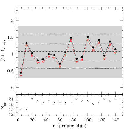
Figure 6: The mean of the $\delta$ field reconstructed around the QSOs in our sample, neglecting the effect of the UV flux from the QSO themselves. The solid dots represent the upper limit case while the open stars trace the lower limit case (see text). The shaded area marks the $3\,\sigma$ region for the upper limit case, the dotted lines mark the corresponding 1 and $2\,\sigma$ levels and the dashed line the average IGM density contrast. The lower panel shows the number of objects contributing to each bin.

Moving closer to the QSO a decrease of the number density of Ly$\alpha$ absorption lines with respect to the mean value is expected.

We applied FLO to recover the density field in the neighbourhood of the QSOs in our sample, deliberately neglecting the contribution of the QSO radiation field to the UV ionising flux. The density field traced by the Ly$\alpha$ forest was computed in each QSO spectrum of our sample. The data were re-binned into bins of 8 proper Mpc in length. Bins covered by more than 33 percent by masked intervals were eliminated from the final count for the single object. Then, in each bin, the mean of all the $\delta$ values contributing to that bin (one per QSO at maximum) was computed. The resulting $\delta$-field is shown in Fig. 6 together with the number of QSOs contributing to each bin. The upper and lower limit case are shown, the difference between the two reconstructions is negligible. The dashed line in the upper panel represents the average of $\delta$ values in the upper-limit case at separations larger than 20 Mpc, no longer affected by the ionising flux from the QSO. The dotted lines are the $1$ and $2\,\sigma$ standard deviations and the shaded region represents the $3\,\sigma$ level. A significant decrease of the density field is observed in the first bin at proper separation from the emitting QSO of less than 8 Mpc, corresponding to the average radius of influence of the QSOs in our sample.

4.1 The density structure around QSOs

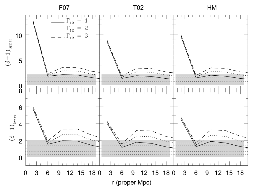
Figure 7: Mean $\delta$ field in the upper (top panels) and lower (bottom panels) limit case in the region close to the emitting QSO (which is located at $r=0.0$) for the QSO spectra in our sample. In each row, the three panels differ for the adopted QSO continuum slope (see Section 3.2). The three curves in each panel differ for the adopted value of $\Gamma_{12}$. The $3\,\sigma$ fluctuations in the IGM region (far away from the QSO) are represented by the shaded area.

In order to recover the density field in the region close to the emitting QSO, its ionising flux has to be added to the UV background, and the total ionisation rate has to be used in eq. 2 of the FLO algorithm. We define $\Gamma_{12}^{\prime}$ as:

$$\Gamma_{12}^{\prime}=\frac{\Gamma_{\rm UVB}+\Gamma_{\rm QSO}}{10^{-12}}$$ (7)

where $\Gamma_{\rm QSO}$ was defined in eq.4. As explained in Section 3.2, the value of $\Gamma_{\rm QSO}$ depends on the adopted slope for the QSO continuum in the region blue-ward of the Lyman limit. We investigated how the three different assumptions for the slope influenced the final result.

In Fig. 7, we present the mean $\delta$ field for the lower and the upper limit case recovered from the spectra in our sample in the region within 20 Mpc from the radiating source in bins of 4 proper Mpc. We studied how the FLO output was modified by assuming different ionisation rates for the UV background, $\Gamma_{12}=1,\ 2,\ 3$, and different slopes for the QSO continuum.

The first important result of our analysis is that FLO recovers the over-density hosting the QSOs in each one of the panels of Fig. 7. The second result is that the value of $\delta$ for the peak varies significantly depending on several factors that are discussed in the following.

1.Treatment of the empty bins:

at variance with the region away from the QSO, the lower and upper limit case in the treatment of the empty bins makes a difference of a factor of $\sim 2$ for the $\delta$ value of the peak of the over-density where the QSO resides. This is due to the QSO strong ionising field that, when applied in eq. 2, transforms even small column densities into large over-densities. Increasing the SNR of our spectra would decrease the minimum detectable H i column density, thus decreasing the difference between the two limiting cases.

2. QSO continuum slopes:

the difference between the two extrapolations with the standard fixed power laws, with indexes $\gamma=1.5$ and 1.8, is $\sim 10$ percent, while there is an increase in the peak value between $\sim 30$ and 45 percent when the F07 slopes are adopted. In the latter model, the continuum in the blue is obtained by extrapolating the slope red-ward of the Ly$\alpha$ emission, so it can be considered as a sort of upper-limit to the true continuum, that cannot be recovered due to contamination by the IGM absorption.

3. Ionisation rate of the UVB:

this parameter does not have any influence on the $\delta$ value for the QSO peak, as expected. On the other hand, the effect on the average value of the $\delta$-field away from the QSO is significant and will be discussed in Section 4.3.

4. QSO systemic redshifts:

the uncertainties in the emission redshifts of the QSOs whose spectrum was used to determine the over-density are of the order of $100-200\ \,{\rm{km\,s^{-1}}}$ corresponding to $\sim 400-800$ proper kpc at $z\simeq 2.5$. As a consequence, we do not expect a major influence on the value of the QSO over-density which is computed in a bin of 4 proper Mpc. A significant improvement in the result would be obtained if the systemic redshift of all the QSOs in the sample would be measured with intermediate resolution spectra in the infrared.

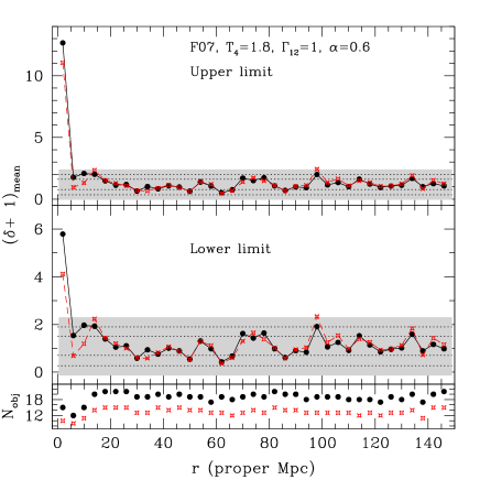
Figure 8: Comparison between the recovered average density field for the total sample (solid dots) and the sample without the QSOs with associated systems (empty stars) in the reference model with the F07 slopes. The shaded regions mark the $3\,\sigma$ interval an the dotted lines the 1 and $2\,\sigma$ level for the reduced sample. In the lower panel the number of objects for the two samples is reported.

5. Associated absorption systems:

metal absorption systems within $\sim 5000$ km s^-1 (corresponding to $\sim 20$ proper Mpc) from the emission redshift of the QSO are defined as associated to the QSO. Some of these systems could indeed be intrinsic to the QSO, that is they could be very close to the emitting region and their position could be determined only by the large velocity at which they were ejected from the QSO itself. Counting these lines as intervening would result in an over-estimate of the density field in the proximity of the QSO. Six QSOs in our sample show associated absorption lines (AAL). Figure 8 reports the comparison between the recovered density field of the total QSO sample and of the sample without AAL for the reference model and the F07 slopes. There is a decrease of $\sim 40$ and $15$ percent in the $\delta$ value of the peak in the lower and upper limit-case, respectively. A slight increase in the scatter of the IGM density field is also measured due to the lower statistics. The point at a separation of 98 Mpc is above the $3\,\sigma$ level, however the fluctuation is due to a single QSO, PKS1448-232 and disappears when the QSO is eliminated from the sample.

4.2 Comparison with previous results

The density distribution in the region close to bright QSOs was studied in two previous works (Rollinde et al., 2005; Guimarães et al., 2007) with a different technique: the variation of the cumulative probability distribution function (CPDF) of the optical depth measured in the Ly$\alpha$ forest region away from and close to the QSO. The advantage of this method with respect to FLO is that the fitting of the lines is not necessary since the observed quantity used is the pixel-by-pixel transmitted flux. On the other hand, before investigating the change of the CPDF with the distance from the QSO, it is necessary to evaluate its evolution with redshift and subtract it. Then, the change in the CPDF has to be translated into a variation of the density field with a bootstrap technique (see Rollinde et al., 2005, for the detailed description).

Rollinde et al. (2005), using a subsample of our sample formed by 12 QSO spectra with $\langle z_{\rm em}\rangle\simeq 2.5$, found a significant over-density for separations between $\sim 3$ and 15 proper Mpc assuming $\Gamma_{12}<3$. They assumed in the computation a QSO continuum with a fixed power law slope $\gamma=0.5$ and a temperature-density relation index $\alpha=0.5$. Guimarães et al. (2007) applied the same technique to a sample of 45 QSO spectra at intermediate resolution and at redshift $\langle z_{\rm em}\rangle\sim 3.8$. An over-density extending to separations of $\sim 15$ proper Mpc is detected adopting the parameters, $\Gamma_{12}=1$, $T_{0,4}=1$, $\alpha=0.0$ and $\gamma=0.7$. These authors claimed also the detection of a correlation between the over-density and the luminosity: brighter QSOs reside in higher over-densities.

The main difference between our result and the previous ones is that we clearly detected an over-density limited to a few Mpc from the QSO, while the results of the optical depth analysis showed a smooth decrease from the peak to the IGM density extending for more than 10 Mpc. In particular, the difference with the result at higher redshift by Guimarães et al. (2007) cannot be ascribed to a difference in QSO intrinsic luminosity, since the average luminosity of the two samples is the same: $\log L_{\rm LL}\simeq 31.7$. We will see in Section 5 that the cosmological hydro-simulations that we used for comparison show very narrow density peaks as found in our recovered density field. Very similar results were obtained by Faucher-Giguère et al. (2008) who investigated with hydrodynamical simulations the bias introduced by the QSO over-density in the estimate of the UV background intensity from the proximity effect. They considered three ranges of masses $3.0\pm 1.6\times 10^{11}$ M${}_{\odot}\ h^{-1}$, $3.0\pm 1.6\times 10^{11}$ M${}_{\odot}\ h^{-1}$ and $6.0\pm 3.2\times 10^{12}$ M${}_{\odot}\ h^{-1}$ for the DM haloes hosting QSOs in the simulations and averaging the results of 100 lines of sight obtained overdensity profiles extending to $\sim 3-5$ proper Mpc at redshifts $z\simeq 2-3$.

4.3 Constraints on the IGM physical parameters

The FLO algorithm depends on the physical parameters of the IGM, in particular the temperature at the average density, the UVB ionisation rate and the index of the temperature-density relation. We adopted for these parameters the values from the cosmological hydro-simulation used to validate the FLO performances in paper I. In turn, these values are in agreement with the most recent observational measurements (e.g. Ricotti et al., 2000; Schaye et al., 2000; Scott et al., 2000; Tytler et al., 2004; Bolton et al., 2005).

In Fig. 7, we showed that values of the UVB ionisation rate $\Gamma_{12}\geq 2$ (corresponding to UVB intensities at the Lyman limit, $\log J_{\rm LL}\geq-21.15$) are rejected at more than $3\,\sigma$ because they over-estimate the average density of the IGM.

We investigated how the variation of the other two relevant parameters, $T_{0,4}$ and $\alpha$, influence the reconstruction of the $\delta$-field with FLO. The results are shown in Fig. 9. A temperature at the average density almost a factor of two lower than the reference one, which implied a decrease in the smoothing scale of $\sim 30$ percent, could reconcile values of $\Gamma_{12}=2$ with the IGM average density but not values as large as $\Gamma_{12}=3$. However, this temperature is at the lowest end of the measured temperatures in the IGM at the considered redshifts. Higher temperatures and high values of $\Gamma_{12}$ allow to recover the correct IGM average density if a lower $\alpha$ index is adopted. In particular, an inverted temperature-density relation with $\alpha\sim-0.5$, as measured by Bolton et al. (2008) from the flux probability distribution function, would require a high temperature, and a high UVB ionisation rate to recover the average IGM density.

However, the validity of the FLO reconstruction with a different set of parameters than the reference one needs to be verified with numerical simulations and we plan to do it in the next paper of the series.

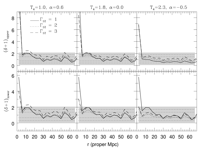
Figure 9: Variation of the FLO output $\delta$-field with the physical parameters of the IGM. The solid line represents the fiducial model with $T_{0,4}=1.8$, $\Gamma_{12}=1$ and $\alpha=0.6$ with the F07 QSO slopes. The dotted and dashed lines are obtained for $\Gamma_{12}=2$ and $\Gamma_{12}=3$, respectively, and varying the temperature and/or the index $\alpha$ as marked above the panels. The shaded regions and the dotted horizontal lines are the same of Fig. 7.

5 Comparison with simulations

We compared the reconstruction of the QSO over-density by FLO with the average density field from a cosmological hydro-simulation in the proximity of the halos that would likely harbour the QSOs in our sample.

5.1 Simulated lines of sight

The simulations were run with the parallel hydro-dynamical (TreeSPH) code GADGET-2 based on the conservative ‘entropy-formulation’ of SPH (Springel, 2005). They consist of a cosmological volume with periodic-boundary conditions filled with an equal number of dark matter and gas particles. Radiative cooling and heating processes were followed for a primordial mix of hydrogen and helium. We assumed a mean UVB produced by QSOs and galaxies as given by Haardt & Madau (1996) with helium heating rates multiplied by a factor 3.3 in order to better fit observational constraints on the temperature evolution of the IGM (Schaye et al., 2000). This background gives naturally a $\Gamma_{\rm UVB}\sim 10^{-12}$ at the redshifts of interest here (Bolton et al., 2005). The star formation criterion is a very simple one that converts in collision-less stars all the gas particles whose temperature falls below $10^{5}$ K and whose over-density is larger than 1000. More details can be found in Viel et al. (2004). The cosmological model corresponds to a ‘fiducial’ $\Lambda$CDM Universe (the B2 series of Viel et al., 2004).

We used $2\times 400^{3}$ dark matter and gas particles in a $120\ h^{-1}$ comoving Mpc box. Having a large box size is crucial since the influence zone of the QSOs is usually of the order of some Mpc or tens of Mpc (see Table 1 of this study). The gravitational softening was set to 5 $h^{-1}$ kpc in comoving units for all particles. We analysed the output at $z=2.2$ and run a Friend-of-Friend (FoF) algorithm to identify the most massive collapsed haloes that should host the QSOs. We found about 400 (54) haloes whose total mass is larger than $2\times 10^{12}$ M${}_{\odot}\ h^{-1}$ (10¹³ M${}_{\odot}\ h^{-1}$). We then pierced the simulated box along the 400 lines of sight (LOSs) intersecting the centre of the haloes with M $\geq 2\times 10^{12}$ M${}_{\odot}\ h^{-1}$ and along random directions. This latter sample constitutes our ‘control’ sample. We explicitly checked that the correlation function of the haloes with masses larger than $2\times 10^{12}$ M${}_{\odot}\ h^{-1}$ is reasonably well fitted by a power-law function with $r_{0}=6\,{\rm{Mpc}}\ h^{-1}$ and slope $-1.8$ in agreement with observational results (Croom et al., 2005). Furthermore, it was recently found that QSOs could be typically hosted in haloes of mass $3\times 10^{12}$ M${}_{\odot}\ h^{-1}$ regardless of their luminosity and redshift (da Ângela et al., 2008).

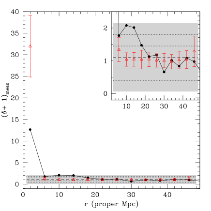
Figure 10: Comparison between the FLO average density field for the observed QSO sample (solid dots, upper limit case) in the reference model with the F07 slopes and the density field from simulations (empty triangles with $1\,\sigma$ error bars). The window in the upper right corner is a zoom of the fluctuations at the mean level. The shaded area marks the $3\,\sigma$ regions, the dotted lines mark the 1 and $2\,\sigma$ and the dashed one the mean density level.

5.2 Comparison of the density fields

For each one of the 400 simulated lines of sight, the density contrast, the temperature, and the peculiar velocity are known pixel by pixel. Peculiar velocities are small, typically less than 100 $\,{\rm{km\,s^{-1}}}$, and randomly oriented. However, since the observed density fields were recovered in redshift space, the mock lines of sight were modified by correcting the redshifts of the density field ($z_{\rm old}$) with the peculiar velocity field to obtain the density field in redshift space ($z_{\rm new}$) using the formula $v_{\rm pec}(z_{\rm old})=c\,(z_{\rm new}-z_{\rm old})/(1+(z_{\rm new}+z_{\rm old})/2)$ and the periodic-boundary conditions. Then, the mock LOSs were shifted (applying the periodic-boundary condition) in order to have the peak of the most massive halo (where the QSO should reside) in the first pixel and the proper separation from this pixel was computed for all the other pixels. The total length of the simulated LOSs is $\sim 50$ proper Mpc. The obtained density fields were finally rebinned into steps of 4 proper Mpc as in the case of the observed ones. The final simulated density field was computed by averaging in each bin the mean $\delta$ of 100 samples of 19 LOSs (the average number of objects per bin in the observed sample) extracted from the total sample of 400 mock LOSs with a bootstrap technique. The error bars on the final density field were computed from the standard deviation of the 100 samples.

The comparison between the simulated density field and the one recovered from observed spectra is plotted in Fig. 10. The simulated $\delta$ field is consistent with the mean IGM density down to 4 Mpc and up to 48 Mpc (see zoomed window). The disagreement between the simulated and observed density contrast in the first bin and, in particular, the large value of $\delta$ obtained from the mock spectra, could be explained by the fact that the considered simulations do not include in the most massive halos the presence of the AGN that would accrete part of the gas in the peak.

6 Conclusions

In this work, we used a sample of $\sim 6300$ Ly$\alpha$  absorption lines obtained from high resolution, high signal-to-noise ratio spectra of 21 QSOs in the redshift range $2.1\lower 2.15277pt\hbox{$\;\buildrel<\over{\sim}\;$}z_{\rm em}\lower 2.15277pt\hbox{$\;\buildrel<\over{\sim}\;$}3.3$ and the FLO algorithm for the reconstruction of baryon density fields (described in details in Paper I) to investigate the baryon distribution as a function of the distance from the QSO.

The effect of the QSO radiation (supposed to be isotropic) dominates over the UV background (UVB) in a sphere with radius varying from $\sim 3$ to 15 Mpc for our sample, with an average of $\sim 8$ Mpc. The increased ionisation flux modifies the local line number density causing the so-called proximity effect, that was used in the past to estimate the intensity of the UVB at the Lyman limit. However, the local line number density is determined not only by the ratio between the UV flux from the QSO and the UVB but also by a variation of the density field due to the fact that QSOs likely lie on density peaks.

The recovery is extremely sensitive to the emission redshift and to the UV flux of the QSOs. We spent a significant effort to obtain, both from the literature and from the spectra at our disposal, the best estimates for the systemic redshifts of the QSOs in our sample in order to reduce the uncertainties to less than $100-200\ \,{\rm{km\,s^{-1}}}$. For the 16 QSOs for which the redshift was determined with $H_{\beta}$, [O iii] (5 QSOs) or with the O i, Mg ii UV emission lines, the average velocity difference with respect to the determinations present in the literature (e.g. Kim et al., 2004, based mainly on the high-ionisation UV lines and Ly$\alpha$ ) is $\sim-500\ \,{\rm{km\,s^{-1}}}$. For the QSO UV flux, we adopted three different models: two with a power law with a fixed slope and one for which each QSO has its own slope obtained from the comparison with a spectral library. The resulting ionisation rates for the three models are within a factor of two.

We improved the performances of FLO with respect of paper I by adopting a smoothing scale $\sim 30$ percent smaller than the Jeans length, following the prescription by Gnedin & Hui (1998). This contrivance allows us to solve the problem of over-estimation of the over-densities we had in paper I and to correctly recover the mean density in the IGM.

We applied the FLO algorithm to each QSO spectrum and recovered the sample-averaged $\delta$ field as a function of the distance from the emitting sources, in bins of 4 proper Mpc. The obtained results are described in the following sections.

6.1 QSO over-density from the proximity effect

i)

If only the UVB ionisation rate is adopted in eq.2 of FLO, neglecting the QSO radiation, a decrease of the mean density field significant at $\sim 2\,\sigma$ is observed within 8 proper Mpc of the emitting QSO, confirming the presence of a proximity effect.

ii)

When also the QSO ionisation rate is taken into account an over-density significant at more than $3\,\sigma$ is recovered at proper separations of less than 4 Mpc (first bin).

iii)

The absolute $\delta$-value of the QSO over-density is uncertain by an overall factor of $\sim 3$. A factor of $\sim 2$ variation is due to the lower and upper-limit $\delta$-value derived for the empty bins during the field reconstructions: corresponding to no absorber or to one absorber with the minimum H i column density detectable in our sample, respectively. This uncertainty can be improved by using more spectra with a larger signal-to-noise ratio. Another factor of $\sim 1.1-1.5$ is due to the different assumptions for the QSO continuum in the region blue-ward of the Ly$\alpha$  emission.

iv)

The uncertainty on the systemic redshift of the QSOs used to determine the density distribution in their neighbourhood is $\lower 2.15277pt\hbox{$\;\buildrel<\over{\sim}\;$}200\ \,{\rm{km\,s^{-1}}}$ corresponding to separations $\lower 2.15277pt\hbox{$\;\buildrel<\over{\sim}\;$}800$ proper kpc. As a consequence, it should have negligible effects on the $\delta$-value of the peak.

v)

We compared the resulting density field with the average density field in the proximity of massive haloes ($M>2\times 10^{12}$ M${}_{\odot}\ h^{-1}$) in a cosmological hydro-simulations. The two distributions are in reasonably good agreement.

vi)

There is a significant discrepancy between our results and the previous determinations of the matter distribution around QSOs, obtained with the optical depth statistics (ODS, Rollinde et al., 2005; Guimarães et al., 2007) at redshifts $\langle z_{\rm em}\rangle\simeq 2.5$ and 3.8. The ODS method recovers gaseous over-densities extending to scales as large as $\sim 15$ Mpc while our overdensity is limited to a region closer than 4 proper Mpc from the QSO. We would need to increase our sample, in particular with QSOs without associated systems in order to study if the brightest objects resides in more extended peaks.

6.2 Constraints on the IGM physical parameters

i)

In the hypothesis of a temperature of the gas at the mean density $T_{0}=1.8\times 10^{4}$ K and an index of the temperature-density relation for the IGM $\alpha=0.6$, an UVB ionisation rate of $\Gamma_{\rm UVB}\simeq 10^{-12}$ s^-1 gives the correct IGM mean density. On the other hand, $\Gamma_{\rm UVB}\simeq 2\times 10^{-12}$ and $3\times 10^{-12}$ s^-1 are excluded at more than 2 and $3\,\sigma$, respectively, because the recovered FLO IGM density field overestimates the mean density.

ii)

Values of $\Gamma_{\rm UVB}>10^{-12}$ s^-1 can be reconciled with the correct IGM mean density if different combination of $T_{0}$ and $\alpha$ are adopted. In particular, an inverted temperature-density relation with $\alpha\simeq-0.5$ used in the FLO algorithm gives the correct IGM mean density for $\Gamma_{\rm UVB}\simeq 3\times 10^{-12}$ s^-1 and $T_{0}\simeq 2.3\times 10^{4}$ K. Such large values of the ionisation rate could arise as a consequence of the He ii reionisation at $z\sim 3$ and of UVB fluctations (e.g. Meiksin & White, 2004). The performances of FLO with different set of parameters than the reference one have however to be tested with numerical simulation. We defer the details of this analysis to a future paper.

6.3 Limiting factors and future developments

i)

Most of the high redshift QSOs have redshifts determined from UV emission lines which are known to be systematically shifted with respect to systemic redshifts. This is particularly critical for proximity effect studies both along and transverse to the line of sight. An improvement in this sense is expected from the new intermediate-resolution, UV to near-IR spectrograph X-Shooter at the VLT (Vernet et al., 2008), that will be operative from the first trimester of 2009.

ii)

The temperature of the IGM gas at the mean density is highly uncertain. Its best determinations date back to 2000, the evidence of a jump in its value at $z\sim 3$ was marginal and should be verified with the present larger samples of high-resolution, high-signal-to-noise QSO spectra. Furthermore, those temperature estimates are used in many cosmological hydro-simulations to re-normalise the ionising background intensity.

iii)

The intensity and nature of the UV background is another unsolved riddle which should require a new observationally-based determination (with the caveat in i) since the present simulations are only now starting to have the resolution and the physics (e.g. the radiative transfer) needed to derive it self-consistently.

References

- Aracil et al. (2004) Aracil B., Petitjean P., Pichon C., Bergeron J., 2004, A&A, 419, 811
- Bajtlik et al. (1988) Bajtlik S., Duncan R. C., Ostriker J. P., 1988, ApJ, 327, 570
- Bechtold (1994) Bechtold J., 1994, ApJS, 91, 1
- Bergeron et al. (2004) Bergeron J., et al., 2004, ESO The Messenger, 118, 40
- Bolton et al. (2005) Bolton J. S., Haehnelt M. G., Viel M., Springel V., 2005, MNRAS, 357, 1178
- Bolton et al. (2008) Bolton J. S., Viel M., Kim T.-S., Haehnelt M. G., Carsweel R. F., 2008, MNRAS accepted, arXiv:0711.2064
- Boroson & Green (1992) Boroson T. A., Green R. F., 1992, ApJS, 80, 109
- Carswell et al. (1982) Carswell R. F., Whelan J. A. J., Smith M. G., Boksenberg A., Tytler D., 1982, MNRAS, 198, 91
- Bryan & Machacek (2000) Bryan G. L., Machacek M. E., 2000, ApJ, 534, 57
- Chand et al. (2004) Chand H., Srianand R., Petitjean P., Aracil B., 2004, A&A, 417, 853
- Corbin (1990) Corbin M. R., 1990, ApJ, 357, 346
- Cristiani & D’Odorico (2000) Cristiani S., D’Odorico V., 2000, AJ, 120, 1648
- Cristiani et al. (1995) Cristiani S., D’Odorico S., Fontana A., Giallongo E., Savaglio S., 1995, MNRAS, 783, 1016
- Croom et al. (2005) Croom S.M. et al., 2005, MNRAS, 356, 415
- da Ângela et al. (2008) da Ângela J., Shanks T., Croom S. M., Weilbacher P., Brunner R. J., Couch W. J., Miller L., Myers A. D., et al., 2008, MNRAS, 383, 565
- Dekker et al. (2000) Dekker H., D’Odorico S., Kaufer A., Delabre B., Kotzlowski H., 2000, SPIE, 4008, 534
- Espey et al. (1989) Espey B. R., Carswell R. F., Bailey J. A., Smith M. G., Ward M. J., 1989, ApJ, 342, 666
- Fan & Tytler (1994) Fan X.-M., Tytler D., 1994, ApJS, 94, 17
- Faucher-Giguère et al. (2008) Faucher-Giguère C.-A., Lidz A., Zaldarriaga M., Hernquist L., 2008, ApJ, 673, 39
- Fioc & Rocca-Volmerange (1997) Fioc M., Rocca-Volmerange B., 1997, A&A, 326, 950
- Fontana & Ballester (1995) Fontana, A., Ballester, P., 1995, ESO The Messenger, 80, 37
- Fontanot et al. (2007) Fontanot F., Cristiani S., Monaco P., Nonino M., Vanzella E., Brandt W. N., Grazian A., Mao J., 2007, A&A, 461, 39
- Fontanot et al. (2006) Fontanot F., Monaco P., Cristiani S., Tozzi P., 2006, MNRAS, 373, 1173
- Gaskell (1982) Gaskell C. M., 1982, ApJ, 263, 79
- Giallongo et al. (1996) Giallongo E., Cristiani S., D’Odorico S., Fontana A., Savaglio S., 1996, ApJ, 466, 46
- Gnedin & Hui (1998) Gnedin N. Y., Hui L., 1998, MNRAS, 296, 44
- Granato et al. (2004) Granato G. L., De Zotti G., Silva L., Bressan A., Danese L., 2004, ApJ, 600, 580
- Guimarães et al. (2007) Guimarães R., Petitjean P., Rollinde E., de Carvalho R. R., Djorgovski S. G., Srianand R., Aghaee A., Castro S., 2007, MNRAS, 377, 657
- Haardt & Madau (1996) Haardt F., Madau P., 1996, ApJ, 461, 20
- Hui & Gnedin (1997) Hui L., Gnedin N. Y., 1997, MNRAS, 292, 27
- Hutchings et al. (1987) Hutchings J. B., Gower A. C., Price R., 1987, AJ, 93, 6
- Kim et al. (2002) Kim T.-S., Carswell R.F., Cristiani S., D’Odorico S., Giallongo E., 2002, MNRAS, 335, 555
- Kim et al. (2004) Kim T.-S., Viel M., Haehnelt M. G., Carswell R. F., Cristiani S., 2004, MNRAS, 347, 355
- Kim, et al. (2007) Kim T.-S., Bolton J. S., Viel M., Haehnelt M. G., Carsweel R. F., 2007, MNRAS, 382, 1657
- Kirkman & Tytler (1997) Kirkman D. & Tytler D., 1997, ApJ, 484, 672
- Komatsu et al. (2008) Komatsu E., Dunkley J., Nolta M. R., Bennett C. L., Gold B., Hinshaw G., Jarosik N. et al. 2008, submitted to APJS, arXiv:0803.0547
- Kulkarni & Fall (1993) Kulkarni V. P., Fall S. M., 1993, ApJ, 413, L63
- Laor et al. (1995) Laor A., Bahcall J. N., Januzzi B. T., Schneider D. P., Green R. F., 1995, ApJS, 99, 1
- Liske & Williger (2001) Liske J., Williger G. M., 2001, MNRAS, 328, 653
- Lu et al. (1991) Lu L., Wolfe A. M., Turnshek D. A., 1991, ApJ, 367, 19
- Meiksin (2007) Meiksin A., 2007, 2007arXiv0711.3358M
- Meiksin & White (2004) Meiksin A., White M., 2004, MNRAS, 350, 1107
- Madau et al. (1999) Madau P., Haardt F., Rees M. J., 1999, ApJ, 514, 648
- Marziani et al. (1996) Marziani P., Sulentic J. W., Dultzin-Hacyan D., Calvani M., Moles M., 1996, ApJS, 104, 37
- McDonald et al. (2001) McDonald P., Miralda-Escudé J., Rauch M., Sargent W. L. W., Barlow T. A., Cen R., 2001, ApJ, 562, 52
- McIntosh et al. (1999) McIntosh D. H., Rix H.-W., Rieke M. J., Foltz C. B., 1991, ApJ, 517, L73
- McLean et al. (2000) McLean B. J., Greene G. R., Lattanzi M. G., Pirenne B., 2000, in ASP Conf. Ser., Vol. 216, 145
- Murdoch et al. (1986) Murdoch H. S., Hunstead R. W., Pettini M., Blades J. C., 1986, ApJ, 309, 19
- Natali et al. (1998) Natali F., Giallongo E., Cristiani S., La Franca F., 1998, AJ, 115, 397
- Nusser & Haehnelt (2000) Nusser A., Haehnelt M., 2000, MNRAS, 313, 364
- Osterbrock (1989) Osterbrock D. E., 1989, Astrophysics of Gaseous Nebulae and Active Galactic Nuclei, University Science Book, Mill Valley, CA
- Rauch et al. (1996) Rauch M., Sargent W. L. W., Womble D. S., Barlow T. A., 1996, ApJ, 467, L5
- Ricotti et al. (2000) Ricotti M., Gnedin N. Y., Shull J. M., 2000, ApJ, 534, 41
- Rollinde et al. (2001) Rollinde E., Petitjean P., Pichon C., A&A, 376, 28
- Rollinde et al. (2005) Rollinde E., Srianand R., Theuns T., Petitjean P., Chand H., 2005, MNRAS, 361, 1015
- Saitta et al. (2007) Saitta F., D’Odorico V., Bruscoli M., Cristiani S., Monaco P., Viel M. 2008, MNRAS accepted, arXiv:0712.2452 (Paper I)
- Schaye et al. (2000) Schaye J., Theuns T., Rauch M., Efstathiou G., Sargent W. L. W., 2000, MNRAS, 318, 817
- Schaye (2001) Schaye J., 2001, ApJ, 559, 507
- Scott et al. (2000) Scott J., Bechtold J., Dobrzycki A., Kulkarni P., 2000, ApJS, 130, 67
- Springel (2005) Springel V., 2005, MNRAS, 364, 1105
- Springel et al. (2005) Springel V., White S. D. M., Jenkins A., Frenk C. S., Yoshida N., et al., 2005 Nature, 435, 629
- Srianand & Khare (1996) Srianand R. Khare P., 1996, MNRAS, 280, 767
- Sulentic et al. (2004) Sulentic J. W., Stirpe G. M., Marziani P., Zamanov R., Calvani M., Braito V., 2004, A&A, 423, 121
- Telfer et al. (2002) Telfer R. C., Zheng W., Kriss G. A., Davidsen A. F., 2002, ApJ, 565, 773
- Tytler (1987) Tytler D., 1987, ApJ, 321, 69
- Tytler & Fan (1992) Tytler D., Fan X.-M., 1992, ApJS, 79, 1
- Tytler et al. (2004) Tytler D., Kirkman D., O’Meara J. M., Suzuki N., Orin A., Lubin D., Paschos P., et al. 2004, ApJ, 617, 1
- Vanden Berk et al. (2001) Vanden Berk D. E., Richards G. T., Bauer A., Strauss, M. A., Schneider D. P., Heckman T. M., York D. G., et al., 2001, AJ, 122, 549
- Vernet et al. (2008) Vernet J., Dekker H., D’Odorico S., Pallavicini R., Rasmussen P. K., Kaper L., Hammer F., Groot P., and the X-shooter team, 2008, ESO Messenger, 130, 5
- Viel et al. (2004) Viel M., Haehnelt M. G., Springel V., 2004, MNRAS, 354, 684
- Viel et al. (2006) Viel M., Haehnelt M. G., Lewis A., 2006, MNRAS, 370, 51L
- Vrtilek & Carleton (1985) Vrtilek J. M., Carleton N. P., 1985, ApJ, 294, 106
- Williger et al. (1994) Williger G. M., Baldwin J. A., Carswell R. F., Cooke A. J., Hazard C., Irwin M. J., McMahon R. G., Storrie-Lombardi L. J., 1994, ApJ, 428, 574
- Wilkes (1986) Wilkes B. J., 1986, MNRAS, 218, 331
- Zaroubi et al. (2006) Zaroubi S., Viel M., Nusser A., Haehnelt M., Kim T.-S., 2006, MNRAS, 369, 734