Dynamics of a vortex domain wall in a magnetic nanostrip: an application of the collective-coordinate approach

Abstract

The motion of a vortex domain wall in a ferromagnetic strip of submicron width under the influence of an external magnetic field exhibits three distinct dynamical regimes. In a viscous regime at low fields the wall moves rigidly with a velocity proportional to the field. Above a critical field the viscous motion breaks down giving way to oscillations accompanied by a slow drift of the wall. At still higher fields the drift velocity starts rising with the field again but with a much lower mobility $dv/dH$ than in the viscous regime. To describe the dynamics of the wall we use the method of collective coordinates that focuses on soft modes of the system. By retaining two soft modes, parametrized by the coordinates of the vortex core, we obtain a simple description of the wall dynamics at low and intermediate applied fields that describes both the viscous and oscillatory regimes below and above the breakdown. The calculated dynamics agrees well with micromagnetic simulations at low and intermediate values of the driving field. In higher fields, additional modes become soft and the two-mode approximation is no longer sufficient. We explain some of the significant features of vortex domain wall motion in high fields through the inclusion of additional modes associated with the half-antivortices on the strip edge.

I Introduction

Dynamics of domain walls in ferromagnetic strips and rings with submicron dimensions is a subject of active research.Allwood et al. (2005); Thomas et al. (2007); Chien et al. (June 2007) This topic is directly relevant to several proposed schemes of magnetic memory and is also interesting from the standpoint of basic physics. The dynamics of domain walls under an applied magnetic field has distinct regimes: viscous motion with a relatively high mobility at low fields and underdamped oscillations with a slow drift at higher fields.Beach et al. (2005)

In a nanostrip, domain wall dynamics is further complicated by the composite nature of the wall which consists of a few – typically two or three – elementary topological defects in the bulk and at the edge of the strip.Tchernyshyov and Chern (2005) As a result, its motion is dominated by a few low-energy degrees of freedom associated with the motion of the topological defects. Weak external perturbations engage only the softest (zero) mode – a rigid translation of the domain wall along the strip. Larger external forces excite additional modes thereby altering the character of motion.

The general approach to the dynamics of composite domain walls was described recently by Tretiakov et al.Tretiakov et al. (2008) The configuration of a domain wall is parametrized by a few collective coordinates $\bm{\xi}=\{\xi_{1},\xi_{2},\ldots,\xi_{N}\}$ representing the soft modes, and the free energy of the system $U$ is treated as a function of $\bm{\xi}$. The Landau-Lifshitz equation for the spin dynamics with damping in Gilbert’s formGilbert (1955, 2004) is translated into a set of coupled equations of motion for the collective coordinates. In a vector notation, they read

$$\mathbf{F}-\Gamma\dot{\bm{\xi}}+G\dot{\bm{\xi}}=0.$$ (1)

Here components of the vector $\mathbf{F}$ are generalized forces $F_{i}=-\partial U/\partial\xi_{i}$ derived from the free energy $U$; the symmetric matrix $\Gamma_{ij}$ characterizes viscous friction; the antisymmetric gyrotropic matrix $G_{ij}$ describes a non-dissipative force of a kinematic origin related to spin precession.

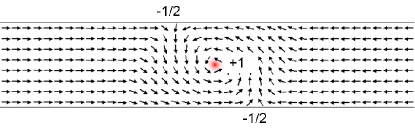
Figure 1: (Color online) A head-to-head vortex domain wall in a long strip of permalloy 200 nm wide. The thickness in the out-of-plane direction is 20nm. Simulation using OOMMF.Donahue and Porter (1999) The winding numbers of the three topological defects are labeled. The shaded region indicates out-of-plane magnetization within the vortex core.

In this paper we describe in detail the application of the collective-coordinate method to the motion of a particular type of domain walls, expanding on our previous report.Tretiakov et al. (2008) Specifically, we focus on vortex domain wallsMcMichael and Donahue (1997) found in long permalloy strips of submicron width $w$ and thickness $t\ll w$. In such a strip, the magnetization pattern is essentially uniform across the thickness, allowing us to consider patterns that vary only along the length (x-direction) and width (y-direction) of the strip.

A vortex domain wall is a magnetization pattern that consists of three topological defects (Fig. 1): a vortex in the bulk of the strip and two half-antivortices confined to the edges.Youk et al. (2006) We will show that the seemingly complex dynamics of a domain wall can be reduced to a simple motion of these defects. The collective-coordinate approach focuses on the soft modes of a system. In the case of a vortex domain wall, the two softest modes turn out to be the coordinate $(X)$ of the vortex core along the long axis of the strip and the coordinate $(Y)$ of the core across the strip width. The dynamic properties of the vortex are similar to that of a massless charged particle moving through a viscous medium in the presence of a potential $U(X,Y)$ and a fictitious magnetic field directed normal to the plane. The “electric charge” of the particle equals $4\pi$ times the topological charge of the vortex,Tretiakov et al. (2008) while the strength of the “magnetic field” equals the two-dimensional spin density.

At low fields the equations describe steady viscous motion of the wall with a velocity proportional to the applied field. The vortex is shifted in the transverse direction by an amount proportional to the velocity of the wall. At a certain critical field the vortex is expelled from the strip and the steady motion breaks down, giving way to an oscillatory regime where the vortex periodically crosses the strip. Each time the vortex comes to an edge it is expelled and reinjected to cross in the opposite direction. At very large magnetic fields one reaches an extreme oscillatory regime, where the vortex quickly moves back and forth across the strip almost along the equipotential lines, while slowly drifting in the direction of the applied field due to viscous forces.

The comparison of the predicted velocity curve to experimentalBeach et al. (2005) and numericalTretiakov et al. (2008) data shows that the theory agrees well with the observations for low fields and fields just above the breakdown. However, the theory predicts a significantly lower drift velocity at high fields than is observed. The origin of the discrepancy has been traced to the appearance of additional soft modes in this regime that are not taken into account in the two-mode approximation. The new modes increase the amount of dissipation in the wall and thereby lead to faster drift.

The paper is organized as follows. In Section II we review the general aspects of the collective-coordinate approach in applications to the dynamics of magnetization. In Section III we derive the equations of motion for the two softest modes of the vortex wall parametrized by the coordinates of the vortex core and discuss the general aspects of their dynamics. A detailed analysis of the dynamics is given in Section IV. The additional soft modes are discussed in Section V. Auxiliary results are derived in the Appendixes.

II Collective Coordinates

II.1 General formalism

The dynamics of magnetization $\mathbf{M}(\mathbf{r},t)$ in a ferromagnet well below the Curie temperature is described by the Landau-Lifshitz-Gilbert equationGilbert (1955, 2004) for the unit vector $\mathbf{m}=\mathbf{M}/M$,

$$\frac{d\mathbf{m}}{dt}=\gamma\mu_{0}\mathbf{H}_{\mathrm{eff}}\times\mathbf{m}+\alpha\mathbf{m}\times\frac{d\mathbf{m}}{dt},$$ (2)

where $\mu_{0}\mathbf{H}_{\mathrm{eff}}(\mathbf{r})=-\delta U/\delta\mathbf{M(\mathbf{r})}$ is an effective magnetic field. The gyromagnetic ratio $\gamma=g|e|/(2m_{e})$ is $1.75\times 10^{11}\mathrm{\ s\,A\,kg^{-1}}$ and the Gilbert damping constant $\alpha\approx 0.01$ in permalloy.Freeman et al. (1998)

The free energy includes, at the very least, exchange and dipolar interactions as well as the Zeeman energy of the ferromagnet in an external field $\mathbf{H}$,

$$U=\int dV\left(A|\nabla\mathbf{m}|^{2}+\mu_{0}H_{\rm{in}}^{2}/2-\mu_{0}\mathbf{H}\cdot\mathbf{M}\right),$$ (3)

where $\mathbf{H}_{\rm{in}}$ is the field induced by the nonuniform magnetization. It satisfies equations $\nabla\cdot(\mathbf{H}_{\rm{in}}+\mathbf{M})=0$ and $\nabla\times\mathbf{H}_{\rm{in}}=0$. The exchange constant in permalloy is $A=1.3\times 10^{-13}$ J/m. Crystalline anisotropy is negligibly small in permalloy; however, such terms can be included in the free energy (3).

In principle, an infinite number of coordinates are necessary to describe the time evolution of a magnetization texture. However, as a domain wall propagates along a nanostrip, much of its structure remains unchanged. While the wall may distort, it retains (at least temporarily) its general shape. For instance, in a vortex wall the chirality of the vortex does not change while the vortex remains within the strip. Likewise, the magnetization far from the wall remains fixed as the wall moves. This suggests that the motion of the wall may be described by a finite set of coordinates $\bm{\xi}=\{\xi_{1},\xi_{2},\ldots,\xi_{N}\}$, so that $\mathbf{m}=\mathbf{m}(\bm{\xi}(t),\mathbf{r})$. In particular, the evolution of magnetization is related to changes in the generalized coordinates as

$$\frac{d\mathbf{m}}{dt}=\frac{\partial\mathbf{m}}{\partial\xi_{i}}\dot{\xi_{i}},$$ (4)

where a sum over the repeated indices is implicit. By substituting Eq. (4) into Eq. (2) and integrating over the volume of the sample, we arrive at the equations of motionTretiakov et al. (2008)

$$F_{i}-\Gamma_{ij}\dot{\xi}_{j}+G_{ij}\dot{\xi}_{j}=0,$$ (5)

with antisymmetric gyrotropic matrix $G_{ij}$ and symmetric matrix of viscosity coefficients $\Gamma_{ij}$. Here

$$F_{i} = -\int dV\,\frac{\delta U}{\delta\mathbf{m}}\cdot\frac{\partial\mathbf{m}}{\partial\xi_{i}}=-\frac{\partial U}{\partial\xi_{i}},$$ (6a)

$$\Gamma_{ij} = \alpha J\int dV~{}\frac{\partial\mathbf{m}}{\partial\xi_{i}}\cdot\frac{\partial\mathbf{m}}{\partial\xi_{j}},$$ (6b)

$$G_{ij} = J\int dV~{}\mathbf{m}\cdot\frac{\partial\mathbf{m}}{\partial\xi_{i}}\times\frac{\partial\mathbf{m}}{\partial\xi_{j}},$$ (6c)

and $J=M/\gamma$ is the density of angular momentum.

Note that $G_{ij}$ obeys the identity

$$\frac{\partial{G_{ij}}}{\partial{\xi_{k}}}+\frac{\partial{G_{jk}}}{\partial{\xi_{i}}}+\frac{\partial{G_{ki}}}{\partial{\xi_{j}}}=0.$$ (7)

If the space of collective coordinates is simply connected, then one may express the gyrotropic tensor in terms of a gauge field $A_{i}$: $G_{ij}=(\partial{A_{j}}/\partial{\xi_{i}})-(\partial{A_{i}}/\partial{\xi_{j}})$. The equations of motion (5) may then be derived from the Lagrangian

$$L=A_{i}\dot{\xi}_{i}-U,$$ (8)

together with the Rayleigh dissipation function $R=\frac{1}{2}\dot{\xi}_{i}\Gamma_{ij}\dot{\xi}_{j}$.

II.2 Soft and hard modes

Equations (5)–(6) are formally exact when they take into account all of the modes of a magnetic texture. If we are not interested in such level of detail, we may focus on a few modes that capture the most salient features of magnetization dynamics and neglect all other modes. It is useful to divide modes into soft ones, which remain active on the typical time scale $T$ of the dynamics, and hard ones, the motion of which decays on a much shorter time scale. Since the drift velocity of a domain wall in an applied magnetic field is ultimately determined by the rate at which its Zeeman energy is dissipated, soft modes with long relaxation times $\tau\gtrsim T$ are responsible for most of the dissipation and thus control the drift velocity. Steady-state motion has an infinite characteristic time $T$, so that only the zero mode – a rigid translation of the wall – with $\tau=\infty$ is relevant in this case. As shown in Sec. III.2, the oscillatory regime has a characteristic time scale $T=\pi/(\gamma\mu_{0}H)$. This regime has one additional soft mode with $\tau_{1}\gtrsim T$ as long as the field is not too strong. As the field strengthens, $T$ becomes shorter and eventually additional modes become soft, $\tau_{2}\gtrsim T$ etc.

A large gyrotropic force creates a softening effect. Consider, as an illustration, system (5) with two modes $\xi_{1,2}$, free energy $U=k(\xi_{1}^{2}+\xi_{2}^{2})/2$, viscosity matrix $\Gamma_{ij}=\Gamma\delta_{ij}$ and gyrotropic matrix $G_{ij}=G\varepsilon_{ij}$, where $\varepsilon_{ij}$ is the antisymmetric tensor with $\varepsilon_{12}=+1$. When $G=0$, one has two purely relaxational modes with $\tau=\Gamma/k$. These modes will be soft for small stiffness $k$ or high viscosity $\Gamma$. In the opposite limit $G\gg\Gamma$ the solution exhibits underdamped oscillations with the relaxation time $\tau=G^{2}/(k\Gamma)$. The latter exceeds the $G=0$ result by a factor $(G/\Gamma)^{2}\gg 1$. We will see that in permalloy, the smallness of $\alpha\approx 0.01$ means that $G\gg\Gamma$, i.e., the gyrotropic force indeed dominates the viscous forces.

The general formalism described in this section is illustrated in Appendix A on the classic problem of a Bloch domain wall first considered by WalkerSchryer and Walker (1974) and recently reviewed by Thiaville and Nakatani.Thiaville and Nakatani (2006)

III Two-coordinate approximation: Generic features

For domain walls under consideration, a large gyrotropic force is associated with the motion of the vortex core (Appendix B). As a result, one may expect the vortex core motion to represent the softest modes of the system, which is indeed the case. We therefore consider a minimal description of the vortex wall with just two coordinates $(X,Y)$ giving the location of the vortex core.Youk et al. (2006) In order to calculate, e.g., the viscosity tensor $\Gamma_{ij}$, we must have a model ${\bf m}={\bf m}(X(t),Y(t))$ for the wall. Such a model is discussed in Appendix C, and the resulting viscosity components for permalloy strips of widths $w=200$ and 600 nm are tabulated in Table 1.

Table 1: Dimensionless ratios $\Gamma_{ij}/G$ for permalloy strips of widths $w=200$ and 600 nm computed for the vortex wall model of Youk et al.Youk et al. (2006) with vortex core placed in the center of the strip. Changing the position of the vortex does not change the results drastically. The ratios depend on the vortex chirality $\chi=\pm 1$.

	$\Gamma_{XX}/G$	$\Gamma_{XY}/G$	$\Gamma_{YY}/G$
$w=200$ nm	0.044	$0.031\chi$	0.049
$w=600$ nm	0.116	$0.103\chi$	0.131

However, once we have settled on the $X$ and $Y$ positions of the vortex core as our collective coordinates, we may draw some general conclusions regarding the motion that are independent of the model we choose for the wall. In particular, this choice of coordinates leads directly to a universal time for the vortex to cross the strip in the transverse direction, in agreement with experimental observations.Hayashi et al. (2007)

III.1 The gyrotropic tensor

Because we are using only the two coordinates of the vortex core to describe the wall motion, the antisymmetric tensor $G_{ij}$ has a single independent component $G_{XY}=-G_{YX}$. As shown in Appendix B, as long as the vortex core is rigid, $G_{XY}$ has a universal value $pG$, where $G=2\pi Jt$, $J=M/\gamma$ is the density of angular momentum, $t$ is the thickness of the film, and the polarization $p=\pm 1$ indicates the sign of the out-of-plane component of the magnetization within the vortex core.

III.2 $X$-dependence of the free energy

A vortex wall with the vortex core at $(X,Y)$ has the free energy $U\approx U(X,Y)$. Because of the translational invariance along the length of the strip, the dependence of the energy on the longitudinal coordinate $X$ at a fixed $Y$ is trivial. A rigid shift of the wall by $\Delta X$ alters the length of the two domains with the opposite magnetizations by $+\Delta X$ and $-\Delta X$ and thus changes the Zeeman energy $-\mu_{0}\int\mathbf{H}\cdot\mathbf{M}\,dV$ by $-QH\Delta X$, where $Q=2\mu_{0}Mtw$ is the magnetic charge of the domain wall (see Appendix C, Fig. 10 in). Hence,

$$U(X,Y)=-QHX+U(Y).$$ (9)

Note that the longitudinal force $F_{X}=-\partial U/\partial X=QH$ is independent of the transverse coordinate $Y$ and in fact of any other details of the wall structure. This has interesting consequences for wall motion in very high magnetic fields. In this limit both gyrotropic and Zeeman forces are much larger than viscous ones, i.e., such a regime corresponds to the limit of zero viscosity. If viscous forces are completely neglected, the longitudinal Zeeman force must balance the longitudinal component of the gyrotropic force $pG\dot{Y}$ giving a constant transverse velocity of the core $\dot{Y}=-pQH/G=-p\gamma\mu_{0}Hw/\pi$ and a universal timeLee et al. (2007); Guslienko et al. (unpublished) for the vortex to cross the strip,

$$T=\frac{w}{|\dot{Y}|}=\frac{\pi}{\gamma\mu_{0}H}.$$ (10)

The transverse coordinate $Y$ thus oscillates at the Larmor precession frequency $\omega_{L}=\gamma\mu_{0}H$. It is a remarkable fact that in zero viscosity limit the same frequency is obtained for a completely different domain wall in Walker’s problem (see Appendix A and Ref. Schryer and Walker, 1974).

III.3 $Y$-dependence of the free energy

In the absence of the applied field the system possesses a symmetry with respect to 180^∘-rotations of the strip, $X\mapsto-X$ and $Y\mapsto-Y$, so that $U(Y)\approx kY^{2}/2$ to the lowest order in $Y$. (Reflectional symmetry $Y\mapsto-Y$ is broken by the chiral nature of the vortex wall.) An applied magnetic field breaks the rotational symmetry allowing a term linear in $Y$. We thus have

$$U(X,Y)=-QH(X+r\chi Y)+kY^{2}/2+\mathcal{O}(Y^{3}),$$ (11)

where $\chi=\pm 1$ is a chirality of the vortex and $r$ is a numerical constant, and $k$ characterizes the restoring force that tries to keep the vortex in the center of the strip. This results in the transverse force $F_{Y}\approx r\chi QH-kY$. The model we use for the vortex wall shows a significant transverse Zeeman force with $r$ of order 1 (see Appendix C, Fig. 10), and nonzero restoring force.

III.4 One-dimensional effective model

In the absence of dissipation, the equations of motion may be derived from the Lagrangian

$$L(X,Y)=-pG\dot{X}Y-U(X,Y).$$ (12)

Note that $\partial L/\partial\dot{X}=-pGY$, so $Y$ is the canonical momentum conjugate to $X$.

If we are interested only in the longitudinal motion of the vortex, we may eliminate the transverse coordinate $Y$ using the equation of motion. In the harmonic approximation for the energy of the wall (11), $Y=(r\chi QH-pG\dot{X})/k$. Substituting this into Eq. (12) gives the effective Lagrangian representing a massive particle in one dimension subject to a constant external force,

$$L(X)=m\dot{X}^{2}/2+QHX,$$ (13)

with the effective mass $m=G^{2}/k$. Using our estimate of the stiffness $k$, Eq. (C.2), and the definition of $G$ in Sec. III.1, one finds that this mass is typically of order $10^{-22}$ kg. This is the same order of magnitude as that found experimentally for a transverse wall by Saitoh et al.Saitoh et al. (2004) and theoretically for a one dimensional wall.Döring (1948); Tatara and Kohno (2004) The mass increases with the width of the strip and changes only weakly with the thickness.

The effective one-dimensional description shall prove useful in Sec. V, where additional degrees of freedom affect the motion of the wall. If these modes also have restoring forces acting on their conjugate momenta, the model becomes one of interacting massive particles in one dimension.

IV Two-coordinate approximation: Dynamics

The equations of motion (5) for two generalized coordinates $\xi_{0}=X$ and $\xi_{1}=Y$ read Tretiakov et al. (2008)

$$F_{i}-\Gamma_{ij}\dot{\xi}_{j}+pG\varepsilon_{ij}\dot{\xi}_{j}=0,$$ (14)

where $\Gamma_{ij}=\Gamma_{ji}$ is the viscosity tensor, $p$ is the polarization of the vortex core, and $\varepsilon_{ij}$ is the $2\times 2$ antisymmetric tensor with $\varepsilon_{01}=+1$. The generalized forces $F_{i}=-\partial U/\partial\xi_{i}$ are derived from the free energy (11). We thus arrive at the following equations of motion for the vortex core:

$$\dot{X} = \frac{QH}{\Gamma_{XX}}+\frac{k(\Gamma_{XY}-pG)}{G^{2}+\det\Gamma}\left(Y-Y_{\mathrm{eq}}\right),$$ (15a)

$$\dot{Y} = \frac{-k\Gamma_{XX}}{G^{2}+\det\Gamma}\left(Y-Y_{\mathrm{eq}}\right),$$ (15b)

where the equilibrium $Y$ position of the vortex is

$$Y_{\mathrm{eq}}=\frac{(\chi g-p)GQH}{k\Gamma_{XX}}$$ (16)

with

$$g=(r\Gamma_{XX}-\chi\Gamma_{XY})/G\ll 1\ .$$ (17)

It is worth noting that the magnitudes of the transverse displacement $|Y_{\mathrm{eq}}|$ are slightly different for the two possible values of the product $p\chi$ of the polarization and the chirality. This effect can be traced to the lack of the reflection symmetry $y\mapsto-y$ in a vortex wall, which leads to nonzero transverse components of the Zeeman force $r\chi QH$ and the viscous force $\Gamma_{YX}\dot{X}$. As a result, the trajectories of vortex cores with the same polarization and opposite chiralities $\chi$ are slightly different.

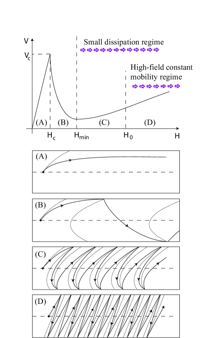
Figure 2: A sketch of the domain wall drift velocity $V(H)$. Lower panels show the vortex motion trajectory (solid lines) and equipotential lines (dotted) at different field magnitudes. (A) - below the Walker breakdown, (B) - just above the Walker breakdown, (C) - small dissipation regime, (D) small dissipation regime with dominating Zeeman force.

Analysis of equations of motion (15) yields three distinct regimes (Fig. 2). Below a critical field $H_{c}$ we find steady viscous motion with a high mobility $\mu=dV/dH$ (see Sec. IV.1 below). Immediately above the critical field $H_{c}$ the vortex motion becomes oscillatory, and the drift velocity of the wall quickly decreases as the applied field grows (see Sec. IV.5 for details). At much higher fields, $H\gg H_{0}=kw/2Q$, the drift velocity rises linearly again but with a much lower mobility $\mu$ than at low fields (Sections IV.3 and IV.4 below). The separation of scales $H_{c}$ and $H_{0}$ is guaranteed by the smallness of parameter $\Gamma_{XX}/G$.

IV.1 Low fields ($H<H_{c}$)

In a low applied field the wall exhibits simple viscous motion. The transverse coordinate of the vortex will asymptotically approach its equilibrium position $Y_{\mathrm{eq}}$, as long as the latter is within the strip. The wall then moves rigidly with a steady longitudinal velocity $V=QH/\Gamma_{XX}$ giving the low-field mobility

$$\mu_{\mathrm{LF}}=dV/dH=Q/\Gamma_{XX}.$$ (18)

Using the calculated value of $\Gamma_{XX}$ (70) for a strip of width $w=600$ nm and Gilbert damping $\alpha=0.01$ yields $\mu_{\mathrm{LF}}=29$ m s^-1 Oe^-1, which is not too far from the value of $25\ \mathrm{m\,s^{-1}\,Oe^{-1}}$ measured by Beach et al. Beach et al. (2005)

IV.2 Critical field ($H=H_{c}$)

As demonstrated in Table 1 and Eq. (70), the viscous force is small in comparison with the gyrotropic one in permalloy strips with a width below 1 $\mu$m. As a result, the equilibrium of a vortex in the transverse direction is set mostly by the balance of the transverse components of the gyrotropic force $GV$ and the restoring force $-kY_{\mathrm{eq}}$. The low-field regime ends when the equilibrium position of the vortex core is pushed beyond the strip edge, $|Y_{\mathrm{eq}}|\geq w/2$, making the steady state unreachable. The critical point is reached when $|Y_{\mathrm{eq}}|=w/2$, so that the critical velocity is

$$V_{c}\approx\frac{kw}{2G},$$ (19)

yielding the critical field

$$H_{c}=\frac{\Gamma_{XX}V_{c}}{Q}=\frac{kw\Gamma_{XX}}{2QG}.$$ (20)

Beach et al.Beach et al. (2005) found a critical velocity of $80$ m/s in a permalloy wire $600$ nm wide. With the aid of Eq. (C.2) for the stiffness constant $k$, we find $V_{c}=188$ m/s in such a wire. This is about twice as high as that observed experimentally. It is, however, much closer than that in Walker’s one dimensional model of the wall, $1770$ m/s.Schryer and Walker (1974); Yang et al. (2008) It is notable that our estimate lies between the experimental measurements and the critical velocity of 256 m/s, found in micromagnetic simulations by Yang et al.Yang et al. (2008)

The critical velocity grows logarithmically with the width of the strip, and nearly linearly with its thickness. It is easy to see that the latter result is valid beyond the model of a vortex wall adopted in this calculation. The two forces balancing each other at $Y_{\mathrm{eq}}=w/2$ scale differently with $t$. While the gyrotropic force is linear in $t$, the restoring force comes from the magnetostatic energy, which represents Coulomb-like interaction of magnetic charges with density $\mathcal{O}(t)$, hence (the dipolar part of) the restoring force is quadratic in $t$ up to logarithmic factors. This implies that $V_{c}$ is roughly proportional to $t$.

IV.3 General remarks for high fields ($H>H_{c}$)

Our numerical simulations in strips of thickness $t=20$ nm and width $w=200$ nm indicate that, after the original vortex with a core polarization $p$ is expelled from the strip, a new vortex is injected at the same location with the opposite polarization $-p$. The vortex thus moves between the edges switching its core polarization each time it reaches an edge.

Once the transverse coordinate of the vortex $Y$ becomes a dynamical variable, the motion acquires an entirely different character. As pointed out above, in permalloy strips the gyrotropic force $G\mathbf{V}$ dwarfs the viscous force $\Gamma\mathbf{V}$. To zeroth order in $\Gamma_{XX}/G$, the dynamics is purely conservative. Using the general form of the Lagrangian (12) one can infer that the vortex core moves along equipotential lines $U(X,Y)=\mathrm{const}$. Absent viscosity, the vortex would oscillate back and forth with the crossing time given by Eq. (10) but the wall would not move on average. Any total $x$-displacement of the wall releases Zeeman energy, and thus requires viscous friction to dissipate it. At a small finite viscosity the vortex trajectory slightly deviates from the equipotential lines, and the wall slowly drifts in the longitudinal direction (Fig. 2 C,D).

IV.4 Very high fields ($H\gg H_{0}$)

We first demonstrate that at very high fields the velocity is again proportional to the field and calculate the high-field mobility for two-coordinate models. The new field scale $H_{0}$ is set by the requirement that the restoring force $-kY$ be negligible in comparison with the Zeeman force $QH$. The characteristic field is

$$H_{0}=\frac{kw}{2Q}=\frac{H_{c}G}{\Gamma_{XX}}\gg H_{c}.$$ (21)

When $H\gg H_{0}$, the dynamics is dominated by the Zeeman and gyrotropic forces, so that the vortex moves almost along an equipotential line $X+r\chi Y=\mathrm{const}$.

As a result of the drift with a velocity $V_{d}$, the Zeeman energy goes down on average at the rate $QHV_{d}$. It is dissipated through heat generated at the rate

$$\mathbf{V}^{T}\Gamma\mathbf{V}=\dot{Y}^{2}\left(\begin{array}[]{cc}-r\chi&1\end{array}\right)\hat{\Gamma}\left(\begin{array}[]{c}-r\chi\\ 1\end{array}\right).$$

The transverse velocity of the vortex core reflects the balance between the longitudinal components of the gyrotropic and Zeeman forces: $\dot{Y}\approx-pQH/G$. We thus find the drift velocity $V_{d}=\mu_{\mathrm{HF}}H$ with the high-field mobility

$$\mu_{\mathrm{HF}}=Q\left(\Gamma_{YY}-2r\chi\Gamma_{XY}+r^{2}\Gamma_{XX}\right)/G^{2}.$$ (22)

The high-field (HF) mobility (22) is suppressed in comparison to the low-field (LF) one (18) by a factor of $\mathcal{O}(\Gamma^{2}/G^{2})=\mathcal{O}(\alpha^{2})$. In the experiment of Beach et al.,Beach et al. (2005) $\mu_{\mathrm{HF}}/\mu_{\mathrm{LF}}\approx 0.1$. Using the $\Gamma$ values for the more realistic model of Youk et al. (shown in Table 1) and $r\approx 2$ as predicted in the Appendix C, we find $\mu_{\mathrm{HF}}/\mu_{\mathrm{LF}}\approx 0.01$. Since the predicted low-field mobility matches the experimental value fairly well (see Sec. IV.1), the calculated high-field mobility is much smaller than the observed value.

IV.5 High fields ($H>H_{c}$): Details

To find the drift velocity of the vortex at fields above the vortex expulsion field $H_{c}$, we determine the total $x$-displacement of the vortex over a full cycle of motion from the top of the strip to the bottom and back again. The crossing time will be slightly different on the upward and downward trips due to a nonzero transverse component of the Zeeman force (Sec. III.3).

Solving Eq. (14) with polarization $p=\pm 1$ gives us the crossing times and displacements $\Delta T_{+}$ and $\Delta X_{+}$ (top to bottom) and $\Delta T_{-}$ and $\Delta X_{-}$ (bottom to top):

$$\Delta X_{\pm} = \frac{QH\Delta T_{\pm}}{\Gamma_{XX}}-\frac{G\mp\Gamma_{XY}}{\Gamma_{XX}}w,$$ (23a)

$$\Delta T_{\pm} = 2\frac{G^{2}+\det\Gamma}{k\Gamma_{XX}}\mathrm{arctanh}\frac{H_{c\pm}}{H},$$ (23b)

where we define $H_{c\pm}=H_{c}/(1\mp\chi g)$, with $g$ defined by Eq. (17). One can see that Eq. (23b) reduces to the universal crossing time of Eq. (10) in the limit $\Gamma_{ij}\to 0$. The drift velocity is

$$V_{d} = \frac{\Delta X_{+}+\Delta X_{-}}{\Delta T_{+}+\Delta T_{-}}$$

$$= V_{c}\left(\frac{H}{H_{c}}-\frac{2(1+\det{\Gamma}/G^{2})^{-1}}{\mathrm{arctanh}(H_{c+}/H)+\mathrm{arctanh}(H_{c-}/H)}\right).$$

Note that the critical fields $H_{c\pm}$ are slightly different reflecting a coupling between the vortex polarity $p$ and chirality $\chi$ seen in Eq. (16).

An expansion of Eq. (LABEL:eq-vd) in powers of $1/H$ yields the high-field result (22). The same expansion allows to find the field $H_{\min}$ at which the domain wall velocity has a minimum:

$$\frac{H_{\min}}{H_{c}}\approx\frac{1}{\sqrt{3(g^{2}+\det\Gamma/G^{2})}}\sim\sqrt{\frac{G}{\Gamma}}\ .$$ (25)

Using expressions (23a) for the displacements $\Delta X_{\pm}$ it is possible to characterize the fields at which the vortex trajectory approaches the zero-dissipation limit. Typical trajectories of the vortex are shown in Fig. 2(C,D). They are close to the equipotential lines $U(X,Y)={\rm const}$ when the displacement $\Delta X_{+}+\Delta X_{-}$ in one back and forth cycle is negligible compared to the strip width $w$. Expansion in $1/H$ gives a criteria

$$\frac{2G}{\Gamma_{XX}}\left(g^{2}+\det\Gamma/G^{2}\right)+\frac{2G}{3\Gamma_{XX}}\left(\frac{H_{c}}{H}\right)^{2}\ll 1$$

or

$$\frac{2G}{\Gamma_{XX}}\left(g^{2}+\det\Gamma/G^{2}\right)\ll 1$$ (26a)

$$\frac{H}{H_{c}}\gg\sqrt{\frac{2G}{3\Gamma_{XX}}}$$ (26b)

For $r\lesssim 1$ the first inequality is always satisfied when $\Gamma\ll G$ holds. Eqs. (25) and (26b) show that vortex motion becomes approximately dissipationless for fields above the velocity minimum.

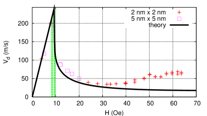
Figure 3: (Color online) The drift velocity $V_{d}$ of the domain wall as a function of the applied field $H$ for a permalloy strip of width $w=200$ nm and thickness $t=20$ nm. Dashed vertical lines mark the critical fields $H_{c-}$ and $H_{c+}$.

In Fig. 3 the predicted drift velocity is compared with the results of numerical simulations for a permalloy strip of width $w=200$ nm and thickness $t=20$ nm.Tretiakov et al. (2008)

The components of the viscosity tensor used are the predicted values for the Youk et al. model listed in Table 1.

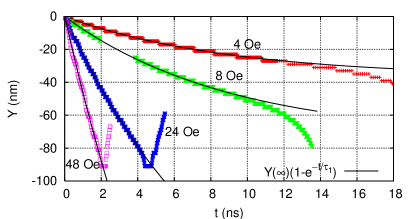
Figure 4: (Color online) The time constant $\tau_{1}$ is determined by fitting the numerically calculated time dependence of the $Y$-coordinate to a decaying exponential, see Eq. (27).

The stiffness constant $k$ of the restoring potential could not be calculated accurately because two of its main contributions, a positive magnetostatic term and a negative term due to Néel-wall tension, are of the same order of magnitude. This is not surprising given the proximity of the strip used in the simulations to a region where the vortex wall is unstable.McMichael and Donahue (1997) Instead, the relaxation time $\tau_{1}=(G^{2}+\det\Gamma)/k\Gamma_{XX}$ was extracted directly from the numerics by fitting $Y(t)$ to the exponential time dependence described by Eq. (15), i.e.

$$Y(t)=Y_{\mathrm{eq}}+[Y(0)-Y_{\mathrm{eq}}]\exp(-t/\tau_{1}),$$ (27)

see Fig. 4. For applied fields from 4 to 60 Oe, $\tau_{1}$ was in the range from 8.5 to 9 ns. This leads to a $k$ value roughly twice that predicted by Eq. (C.2). In accordance with Eq. (15), the equilibrium position $Y_{\mathrm{eq}}$ scales linearly with $H$. In calculating the critical velocity $V_{c}=kw/(2G)$, it was necessary to replace $w$ with an effective strip width $w_{\mathrm{eff}}=w-2R_{0}$ to account for a finite size of a vortex coreWachowiak et al. (2002) and edge defect. As the vortex approaches the edge, the short-range attractive exchange interaction overwhelms the dipolar potential and draws the vortex into the edge defect. This leads to a deviation of the transverse vortex coordinate plotted in Fig. 4 from Eq. (27) as the vortex comes close to the edge. From the observed trajectories we estimated $R_{0}\approx 10$ nm.

V Beyond the two-coordinate approximation

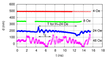
Figure 5: (Color online) Numerical simulations above the critical field show repeated oscillations in the width of the wall, measured as the distance between the half-antivortices. The patterns for various field values are offset vertically by 150 nm for clarity. Each wall width is oscillating near $w=200$ nm. The vortex crossing time $T$ and the decay time of wall width oscillations $\tau_{2}$ are shown by arrows.

At low and intermediate fields, the two-coordinate model shows good agreement with numerical simulations. However, in higher fields the calculated drift velocity falls below the value observed in the numerics (Fig. 3). The discrepancy is caused by the softening of additional degrees of freedom that have so far been ignored. The new soft modes provide additional channels for the dissipation of Zeeman energy leading to an increase in the velocity. In fields above $H_{2}=35$ Oe, the oscillation period $T=\pi/(\gamma\mu_{0}H)$ becomes comparable to the decay times $\tau$ of some of the harder modes. The new modes can be seen in oscillations of the total width of the wall that occur after the vortex has been absorbed by the edge and reemitted (Fig. 5). Including additional modes in the calculation clarifies some of the significant features of the wall dynamics observed in numerical simulations at high fields.

We first present a hypothetical toy model with two additional degrees of freedom in Sec. V.1. It provides a pedagogical example of coupled hard and soft modes with gyrotropic forces and sets the stage for a more realistic model with six degrees of freedom appropriate for a vortex domain wall in higher fields, which is the subject of Sec. V.2.

V.1 Pedagogical model with 4 coordinates

The high-frequency oscillations of a vortex wall (Fig. 5) can be reproduced in a simple phenomenological model where the wall is treated as a vortex-antivortex pair with cores located at $(x_{1},y_{1})$ and $(x_{2},y_{2})$. (A real vortex wall contains a vortex and two half-antivortices.Tchernyshyov and Chern (2005)) The gyrotropic tensor of the system has the following nonzero components:

$$G_{x_{1}y_{1}}=-G_{y_{1}x_{1}}=G_{1},\quad G_{x_{2}y_{2}}=-G_{y_{2}x_{2}}=G_{2}.$$ (28)

Both defects are confined in the transverse direction and coupled to each other in the longitudinal direction with an equilibrium separation $a$. They carry magnetic charges $Q_{1}$ and $Q_{2}$. The potential energy of the system is

$$U=\sum_{i=1}^{2}\left(\frac{k_{i}y_{i}^{2}}{2}-HQ_{i}x_{i}\right)+\frac{k(x_{1}-x_{2}-a)^{2}}{2}.$$ (29)

The Lagrangian is

$$L=-G_{1}\dot{x}_{1}y_{1}-G_{2}\dot{x}_{2}y_{2}-U.$$ (30)

In this pedagogical example we assume that the viscous force acts on the antivortex only, so that the dissipation tensor has a single nonzero component $\Gamma_{x_{2}x_{2}}=\Gamma>0$, giving rise to the Rayleigh dissipation function $R=\Gamma\dot{x}_{2}^{2}/2$. Also, it is important to note that the vortex core is flipped whenever it reaches the edge of the strip, $y_{1}=\pm w/2$, altering the sign of $G_{1}$.

V.1.1 Two massive particles

It is instructive to eliminate the transverse coordinates $y_{1}$ and $y_{2}$, as in Sec. III.4, using the equations of motion, $k_{i}y_{i}=-G_{i}\dot{x}_{i}$. The resulting dynamics is that of two massive particles moving in one dimension. The potential energy of the original model (29) translates into a sum of kinetic energy $K$ and potential energy $U$ of the massive particles:

$$E = K+U$$

$$= \frac{m_{1}\dot{x}_{1}^{2}}{2}+\frac{m_{2}\dot{x}_{2}^{2}}{2}+\frac{k(x_{1}-x_{2}-a)^{2}}{2}-H(Q_{1}x_{1}+Q_{2}x_{2}),$$

where the masses are determined by the gyrotropic and stiffness constants, $m_{i}=G_{i}^{2}/k_{i}$. Continuous evolution of the system is disrupted when the velocity of the vortex attains a critical magnitude, $|\dot{x}_{1}|=v_{c}=k_{1}w/2G_{1}$, signaling that the vortex has reached the edge. At that moment $G_{1}$ changes sign and the longitudinal vortex velocity $\dot{x}_{1}=-k_{1}y_{1}/G_{1}$ is reversed, $\dot{x}_{1}\to-\dot{x}_{1}$. After that continuous evolution resumes. Nothing special happens to the antivortex at that moment.

The natural modes of the system are the center of mass $X=(m_{1}x_{1}+m_{2}x_{2})/M$ and relative position $x=x_{1}-x_{2}-a$. Their energies are

$$E_{\mathrm{CM}} = \frac{M\dot{X}^{2}}{2}-QHX,$$ (32a)

$$E_{\mathrm{rel}} = \frac{\mu\dot{x}^{2}}{2}+\frac{kx^{2}}{2}-qHx,$$ (32b)

where $M=m_{1}+m_{2}$ and $\mu=(m_{1}^{-1}+m_{2}^{-1})^{-1}$ are the total and reduced masses and $Q=Q_{1}+Q_{2}$ is the total magnetic charge. The value of the relative magnetic charge $q$ will not matter to our analysis.

We consider the limit in which the antivortex is strongly confined in the transverse direction, so that $k_{2}\gg k_{1}$ and as a result, the antivortex is much lighter than the vortex,

$$M\sim m_{1}\gg m_{2}\sim\mu.$$ (33)

Here we rely on the fact that the gyrotropic coefficients of the vortex and the antivortex have the same magnitude, see Appendix B.

The center-of-mass position $X$ is a zero mode with an infinite relaxation time. Its velocity $\dot{X}$ is an overdamped mode with the relaxation time $\tau_{1}\sim m_{1}/\Gamma=G_{1}^{2}/(k_{1}\Gamma)$, which is essentially the same as in our two-coordinate model of the vortex wall. The remaining two modes represent underdamped oscillations of the relative coordinate and velocity with the frequency $\omega\sim\sqrt{k/\mu}$ and relaxation time $\tau_{2}\sim 2m_{2}/\Gamma\ll\tau_{1}$. Thus $x$ and $\dot{x}$ are much harder than $X$ and $\dot{X}$ and there is a regime, $\tau_{1}\gg T\gg\tau_{2}$, where we may neglect the relative motion as a hard mode. In that regime, the dynamics of the wall reduces to that of our simple two-mode model described in Sec. IV.

V.1.2 Losses from the hard modes

Let us compare the energy losses from the soft and hard modes to check whether our neglect of the hard modes is justified. In the limit $\tau_{2}\ll T$, the relative position $x$ and velocity $\dot{x}$ quickly reach their equilibrium values retaining them through most of the crossing period $T$. However, as the velocity of the vortex $\dot{x}_{1}$ reverses its sign, the relative velocity $\dot{x}=\dot{x}_{1}-\dot{x}_{2}$ changes as well increasing from zero to $\pm 2v_{c}$. The energy of relative motion increases by $2\mu v_{c}^{2}$ at the expense of the center-of-mass energy. (Note that the total energy (LABEL:eq-E) does not change at all since it is not sensitive to the sign of $\dot{x}_{1}$.) The kinetic energy of relative motion $2\mu v_{c}^{2}$ will be fully dissipated during the initial stage of the next crossing.

The energy lost by the oscillatory relative motion, $\Delta E_{2}=2\mu v_{c}^{2}$, should be compared to the total loss incurred primarily through the overdamped main mode,

$$\Delta E=\int_{0}^{T}\Gamma\dot{x}_{2}^{2}dt\sim\int_{0}^{T}\Gamma\dot{X}^{2}dt\sim\frac{\Gamma v_{c}^{2}T}{3}.$$ (34)

The fraction of energy dissipated through the hard modes is thus

$$\frac{\Delta E_{2}}{\Delta E}\sim\frac{3\tau_{2}}{T}.$$ (35)

As long as relative motion remains hard, $\tau_{2}\ll T$, energy loss associated with it is negligible and the motion of the system is well approximated by the soft modes $X$ and $\dot{X}$ alone.

V.2 Model with 6 coordinates

Transient oscillations of the hard modes found in the pedagogical model are similar to the oscillations of the width of the vortex wall (Fig. 5), measured as the distance between the two edge defects. In our numerical simulations, after the vortex is absorbed and reemitted at the edge, the width of the wall displays underdamped oscillations. In moderate fields, these oscillations decay during the crossing time $T$ and are reactivated at the beginning of the next cycle. This activation is evidence of energy transfer from the vortex core to harder modes, just as occurred in the pedagogical model of Sec. V.1. In sufficiently high fields, the vortex crossing time $T=\pi/(\gamma\mu_{0}H)$ becomes comparable to the relaxation time of the new modes. Notably, this occurs in the same region of field strength in which the two-coordinate model prediction for the drift velocity begins to deviate from the results of numerical simulations (Fig. 3). New dissipation channels become important in higher fields, changing the dynamics of the wall.

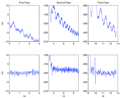
Figure 6: (Color online) Top row: The left hand side of Eq. (37) for the two-coordinate model plotted for the first three passes of the vortex across the strip under an applied field of 32 Oe. Bottom Row: When a finite mass $m=1.1\times 10^{-23}$ kg is included for the edge defects, as in Eq. (47), the total $x$-momentum of the modes is conserved.

Further evidence of the need to include additional modes may be gleaned by comparing the equations of motion of the two-coordinate model to the numerical simulations directly. The two-coordinate model predicts that

$$-pG\dot{Y}=QH-\Gamma_{XX}\dot{X}.$$ (36)

This equation expresses the change of linear momentum in the $x$ direction due to external forces, and holds while the vortex is inside the strip. Indeed, the momentum canonically conjugate to coordinate $X$ is $\partial L/\partial\dot{X}=-pGY$ (12). As a consequence of the translational invariance of the strip in the $x$ direction, this momentum is influenced only by forces external to the wall, i.e. the driving force $QH$ from the field and the drag force $-\Gamma_{XX}\dot{X}$. Equation (36) may be integrated to yield

$$\frac{\Gamma_{XX}}{G}X-pY-\frac{QH}{G}t=\mathrm{const}$$ (37)

The above holds while the vortex is crossing the strip. Formally Eq. (37) does not describe the collision with the edge, but it can be checked that the effect of collision and corresponding vortex polarization flip is captured by a change of constant on the right hand side of Eq. (37) by $\mathrm{const}\to\mathrm{const}\pm w$.

We can test this prediction using numerical simulations. The value of the left-hand-side of this equation is plotted in the top row of Fig. 6 for the first three passes of the vortex across a 200-nm-wide, 20-nm-thick strip when a 32-Oe driving field is applied. For $\Gamma_{XX}$, we use the theoretical estimate $\Gamma_{XX}=0.044G$ for the model of Youk et al. (Table 1). In the two-mode approximation, the plotted value should be constant during each pass. However, it is clearly not constant and displays oscillations reminiscent of those in the wall width (Fig. 5).

Equation (37), derived in the two-mode approximation states that momentum along the nanostrip is influenced only by two external forces. Its violation reflects a transfer of momentum between the vortex and other modes of the wall. In a model with a larger number of modes a similar equation on the x-direction momentum can be derived and checked numerically. It provides a good test showing whether the new set of modes is sufficient to capture the actual wall motion.

The evidence in Fig. 5 and Fig. 6 shows that the modes associated with the positions of the edge defects become important to the motion of the wall in intermediate to high fields. We add the coordinates of these defects to our description in order to explain qualitatively their behavior as observed in numerical simulations. We use some simple modeling for the forces holding the edge defects in place relative to the vortex core. As with the vortex itself, each edge defect is described by two coordinates that are coupled to one another through the gyrotropic tensor. In the case of the vortex, these two variables are the $X$ and $Y$ coordinates of the core. For the edge defects, we use the $X$-positions $X_{\pm}$ of the defects and the out-of-plane angles $\theta_{\pm}$ of the magnetization at their cores. It is not surprising that a gyrotropic coupling should be present between these coordinates, as it is the same pairing that occurs in Walker’s problem of the Bloch wall—see Appendix A for details.

V.2.1 Energy

In order to describe the motion of the two edge defects, two springs are added to the energy $U(X,Y)$ in Eq. (11) that act to keep the upper $(X_{+})$ and lower $(X_{-})$ edge defects on a $45^{\circ}$ line with the vortex

$$U_{e\pm}=\frac{k_{2}}{4}\left(X+\chi Y-X_{\pm}\mp\frac{\chi w}{2}\right)^{2}.$$ (38)

Here again $\chi$ is the chirality of the vortex. (Which of the two edge defects is ahead of the vortex depends on the vortex chirality.)

To take into account the energy cost of bringing magnetization out of the plane of the strip near the edge defects, the restoring springs are added for the angles $\theta_{+}$ and $\theta_{-}$ associated with the upper and lower edge defects, respectively:

$$U_{\theta\pm}=\frac{k_{\theta}}{2}\theta_{\pm}^{2}.$$ (39)

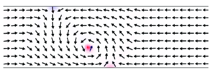
Figure 7: (Color online) Image of a wall moving to the right with an applied field of 4 Oe. Shaded regions indicate out-of-plane magnetization.

To represent the gyrotropic coupling of the positions of the edge defects to their out-of-plane angles, the terms

$$L_{\pm}=\mp G_{2}\dot{X}_{\pm}\theta_{\pm}$$ (40)

are added to the Lagrangian.

The gyrotropic coefficients for the upper and lower edge defects have opposite signs because they wind in opposite directions as one moves from left to right. This effect is visible in simulations even below the first breakdown field (Fig. 7). As the wall moves to the right at a steady velocity, the lower defect tilts up out of the plane, while the upper defect tilts into the plane.

The total Lagrangian for this extended model is then

$$L=-pG\dot{X}Y-U(X,Y)+\sum_{b=\pm}(L_{b}-U_{eb}-U_{\theta b}),$$ (41)

where $U(X,Y)$ is given by Eq. (11).

V.2.2 Viscosity

It remains to determine the components of the viscosity tensor for the three defects. Under the assumption that the three defects may move independently of one another, it is logical to assume that the viscosity tensor $\Gamma$ will be essentially diagonal. Each of the edge defects carries with it a portion of the wall, and that portion’s associated viscosity. Since the vortex is moving independently of the edge defects, there is no asymmetry that would lead to off-diagonal terms. The most general (second order) Rayleigh dissipation function consistent with these conditions is:

$$R=\frac{1}{2}\sum_{i}\Gamma_{i}\dot{\xi_{i}}^{2},$$ (42)

where $\Gamma_{X_{+}}=\Gamma_{X_{-}}=\Gamma_{e}$, and $\Gamma_{\theta_{+}}=\Gamma_{\theta_{-}}=\Gamma_{\theta}$. The largest dissipation component is expected to come from the $X_{\pm}$ positions of the half-antivortices, as they influence the motion of the Néel walls that emanate from them (see Fig. 11). These Néel walls carry most of the viscosity of the wall, as they are the regions where the magnetization changes most rapidly with position. According to Eq. (6b), the viscous tensor components have the largest contribution from the regions where the change of magnetization with the coordinate is the largest. The smallest dissipation component is expected to be that associated with the out-of-plane angles of the edge defects. These angles influence only a small region of magnetization immediately around the cores of the half-antivortices, and so will not have large contributions to the integral in Eq. (6b). Therefore, we ignore $\Gamma_{\theta}$ in what follows.

V.2.3 Connection with the two-mode approximation

This model can be related back to the model in which only the vortex is free to move by letting $k_{2}\rightarrow\infty$ and $k_{\theta}\rightarrow\infty$. This will require $X_{+}+X_{-}=X+\chi Y$, $-\chi(X_{+}-X_{-})=w$, and $\theta_{+}=\theta_{-}=0$ for all time, leading to the reduced Lagrangian and Rayleigh function for just the vortex position:

$$L_{v} = -pG\dot{X}Y-U(X,Y),$$ (43a)

$$R_{v} = \Gamma_{X}\dot{X}^{2}/2+\Gamma_{Y}\dot{Y}^{2}/2+\Gamma_{e}\left(\dot{X}+\chi\dot{Y}\right)^{2}.$$ (43b)

Identifying $\Gamma_{X}=\Gamma_{XX}-\chi\Gamma_{XY}$, $\Gamma_{Y}=\Gamma_{YY}-\chi\Gamma_{XY}$, and $\Gamma_{e}=\chi\Gamma_{XY}/2$, these are exactly the functions used when only the components of the vortex position are soft modes (Sec. IV). It becomes clear then that the off-diagonal elements of the viscosity tensor in the 2-mode model arise directly from the asymmetric equilibrium positions of the edge defects. By comparing the identifications above with the viscosity values in Table 1 and Appendix C, one can see that $\Gamma_{e}$ is indeed the dominant viscosity term, especially as the width increases.

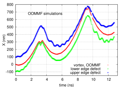
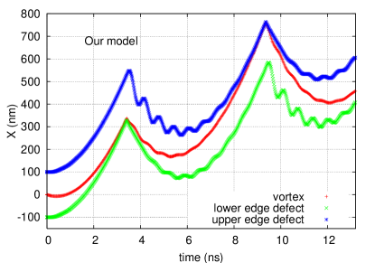
Figure 8: (Color online) Top: Numerically determined $x$-positions of the vortex and the two half-antivortices in a 20 nm thick, 200 nm wide permalloy strip as functions of time for $H=32$ Oe. Bottom: The longitudinal positions of the vortex and the two half-antivortices in the model with massive edge defects. The vortex merges with an edge defect each time it hits the edge. Note that the oscillation of that edge defect is suppressed compared to the other.

Now that we have determined the viscosity values for the new model in terms of the old one, we can check the descriptive value of the model by testing the conservation of the total momentum in the numerical data. This momentum is derived in the next section.

V.2.4 Mass and momentum of the edge defects

If we care only about the $x$-positions of the edge defects, we may integrate out the values of $\theta_{\pm}$ as in Sec. III.4 to produce masses $m=G_{2}^{2}/k_{\theta}$ for the edge defects. The parameters $k_{\theta}$ and $G_{2}$ then appear only in this combination. In effect, these masses occur because the moving wall is able to store kinetic energy in the out-of-plane angle of the edge defects. The Lagrangian then becomes:

$$L=-pG\dot{X}Y-U(X,Y)+\sum_{b=\pm}(m\dot{X}_{b}^{2}/2-U_{eb}).$$ (44)

The total $x$-direction momentum is then equal to

$$P_{x}=-pGY+m(\dot{X}_{+}+\dot{X}_{-})$$

It is influenced by two forces in the $x$-direction. First, viscous drag acts on each of the defects, totaling to

$$F_{d}=-\Gamma_{X}\dot{X}-\Gamma_{e}\dot{X}_{+}-\Gamma_{e}\dot{X}_{-}.$$ (45)

Second, the external field applies a constant force $F_{H}=QH$ on the wall.

As in the two coordinate model, the translational invariance of the system implies that the internal forces between the defects will have no influence over the total $x$ momentum. Note in particular that the analysis here is independent of the spring constants $k$ and $k_{2}$. Thus

$$\frac{dP_{x}}{dt}=F_{d}+F_{H},$$ (46)

This equation may be integrated to yield

$$P_{x}+\Gamma_{X}X+\Gamma_{e}\left(X_{+}+X_{-}\right)-QHt=\mathrm{const}.$$ (47)

We may determine the mass of the edge defects by fitting the left-hand side of Eq. (47) to a constant. The left-hand side of this equation divided by the gyrotropic constant $G$ is plotted in the bottom row of Fig. 6. The figure shows that Eq. (47) with $m=1.1\times 10^{-23}$kg is satisfied by the numerical simulation at 32 Oe to nearly the accuracy of our simulation, which had a 2 nm cell size.

V.2.5 Oscillations of the wall width

Insight into the width oscillations can be gained immediately from the form of $L$ and $R$ in Eqs. (41) and (42). Defining the wall width $d$ by the difference $-\chi(X_{+}-X_{-})$ between the forward and rear edge defects reveals that the conjugate pair $(d,\bar{\theta})$, where $\bar{\theta}=(\theta_{+}+\theta_{-})/2$, decouples from the remainder of the motion. Any deviation in $d$ from $w$ will decay over time with a time constant $\tau_{d}=2m/\Gamma_{e}$, while oscillating due to the gyrotropic coupling with the average out-of-plane angle of the defects.

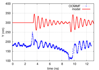
Figure 9: (Color online) Oscillations in the width of the wall in a strip with thickness $t=20$ nm and width $w=200$ nm in a field of $H=32$ Oe. The upper curve shows the prediction of the model using the same parameters as in Fig. 8. It is offset vertically by 100 nm from the numerically determined result for clarity.

The equations of motion associated with the system described above can be solved to find the trajectories of the three defects. In order to take the collisions of the vortex with the edges of the strip into account, the polarization of the vortex is flipped every time it hits the edge. The effective width $w_{\rm{eff}}=w-2R_{0}$, with $R_{0}=10$ nm, is used to account for the short-range exchange interaction of the vortex with the edge. The polarization flip changes the sign of the momentum of the vortex, as in Sec. V.1.1. In addition, when the vortex hits an edge, it actually must collide with one of the edge defects to be absorbed. The vortex is reemitted from that defect with the opposite polarization. As a result, the polarization of the edge defect changes as well. This causes oscillations in the wall width $d$ not because $d$ itself has changed, but because its conjugate momentum $\bar{\theta}$ has been altered.

The solution shown in Fig. 8 and Fig. 9 uses a crude method to demonstrate this effect, simply reversing the value of the out-of-plane angle of an edge defect whenever a vortex hits it. Thus the vortex and the edge defect that it hits both have their momentum change sign during the collision. This is similar to the effect discussed in Sec. V.1.1, in that it causes a sudden transfer of energy from the main mode, associated with the vortex motion, to ancillary modes associated with the oscillation of the edge defects. This effect is seen in Figs. 5 and 9, as the wall oscillation is reactivated every time the vortex hits the edge of the strip.

The $x$ coordinates of the three topological defects over time are plotted in Fig. 8 for the numerical solution and for the model in this section. The parameters used for the model are: $G^{2}/(k\Gamma_{XX})=8.75$ ns as measured in Fig. 4, $m=1.1\times 10^{-23}$ kg as determined in Fig. 6, $r=1.1$ to match the points where the vortex hits the wall, and $k_{2}/k=1.3$ to match the frequency of oscillations.

The oscillations in the positions of the edge defects in the model and numerical solutions are comparable. In particular, the model correctly captures the fact that the oscillations in the farther edge defect from the vortex are larger in amplitude than those of the nearer one. This comes from the combination of flipping the sign of the vortex momentum with the resetting of the angle of the impacted edge defect. The oscillations caused by each effect interfere with one another. This interference is destructive for the near defect and constructive for the far one.

Figure 9 shows the oscillations in the width of the wall. As expected, these oscillations have the largest amplitude immediately after the vortex is emitted from one of the walls. The time constant of the decay is of the same order in both the model and numerical solutions. This agreement for the decay constant $\tau_{d}=2m/\Gamma_{e}$ is expected, since this constant depends only on the edge defect mass measured in Fig. 6 and the viscosity coefficient $\Gamma_{e}$, which is known from the two-coordinate model.

However, Fig. 9 also reveals the limitations of the model described in this section. While this model is useful in explaining the oscillations of edge defects, and the choice of coordinates shows excellent agreement with the $x$-momentum equation (47), as shown in Fig 6, there is still a significant discrepancy between the the theoretical prediction and the numerical simulation in Fig. 9. The average wall width seen in numerical simulations changes as the vortex crosses the strip, an effect that is not predicted by the theory thus far. To account for this effect, additional terms must be added to Lagrangian (41). In particular, this model thus far has ignored field-dependent contributions to the interactions between the defects, as well as terms of higher than quadratic order in the coordinates.

VI Discussion

We have explored the dynamics of a vortex domain wall in a magnetic strip of submicron width. We have applied the method of collective coordinatesTretiakov et al. (2008) to the case when the wall has two soft modes related to the motion of the vortex core. A simplified model of the vortex domain wall described in this paper yields solvable equations of motion. The calculated mobility of the wall in the steady-state viscous regime at low fields agrees well with the value measured by Beach et al.Beach et al. (2005) The steady motion breaks down when the equilibrium position of the vortex moves beyond the edge of the strip. The critical velocity depends strongly on the magnetization length and the sample thickness, and weakly on the width; its calculated value agrees reasonably well with the data of Beach et al.Beach et al. (2005) The dynamics above the breakdown changes its character from overdamped to underdamped. In this regime the velocity sharply declines at first but later starts to rise again as the field strength increases. The predicted high-field mobility is reduced in comparison with the low-field value by the factor $\mu_{\mathrm{HF}}/\mu_{\mathrm{LF}}\approx 0.01$; the experimentally observed reduction is not as strong: $\mu_{\mathrm{HF}}/\mu_{\mathrm{LF}}\approx 0.1$.Beach et al. (2005)

We have compared the results of our theory to numerical simulations of a moving vortex wall in a permalloy strip of width $w=200$ nm and thickness $t=20$ nm. We have found that the results obtained via the collective-coordinate method are in quantitative agreement with the simulations both in the viscous regime at low applied fields and in the oscillatory regime at moderately high fields. As the field strength increases further, the velocity observed in numerical simulations diverges from the predictions of the two-coordinate model. We have traced the breakdown of the two-mode theory to the appearance of four additional soft modes associated with the coordinates and out-of-plane angles of the edge defects (antihalfvortices).

As expected, the dynamics of a domain wall reduces to the motion of the elementary topological defects that make up the wall—bulk vortices and halfvortices at the edge. Of particular importance is the special kinematics of vortices caused by their nonzero skyrmion numbers ($\pm 1/2$). On the formal level, the two coordinates of a vortex core form a canonically conjugated pair. As a consequence, when the vortex is constrained in the transverse direction by a parabolic potential, its longitudinal motion acquires inertia. By our estimates, in a strip of width $w=200$ nm and thickness $t=20$ nm a vortex wall has an effective mass of approximately $10^{-22}$ kg. The mass of an edge defect is approximately $10^{-23}$ kg. Saitoh et al.Saitoh et al. (2004) determined the mass of a transverse wall in 70nm wide, 45nm thick permalloy to be $6.6\times 10^{-23}$ kg.

In our analysis, we have made some simplifying assumptions that require further investigation. First, we have assumed that any vortex absorbed by the edge is immediately reemitted. While this holds true for our simulated strips of $w=200$ and $t=20$ nm, it is not always the case. There may be short delays between absorption and reemission during which the wall motion is again viscous; the higher mobility during this period would tend to increase the drift velocity. This type of motion has been observed in simulations of thinner strips by Lee et al.Lee et al. (2007)

Second, while we have described the onset of wall width oscillations in Sec. V as a typical new mode, decaying oscillations are not the only type of new mode that can occur. In particular, the number and dynamic characteristics of soft modes may change discontinuously as additional vortices or antivortices are created in the bulk of the strip.Guslienko et al. (2008) We have observed numerically the creation and subsequent annihilation of a vortex-antivortex pair adjacent to the original vortex of the wall. As in the process described by Van Waeyenberge et al.,Van Waeyenberge et al. (2006) the pair creation mediates the flipping of the polarization of the vortex and results in the reversal of the gyrotropic force. Once the pair is created, the antivortex moves closer to the original vortex and together they form a topologically non-trivial bound state (a skyrmion) of the type described in detail by Komineas,Komineas (2007) eventually decaying in a spin wave explosion via a quasi-continuous process in which the conservation of topological charge is violated.Hertel and Schneider (2006); Tretiakov and Tchernyshyov (2007) The new vortex, which has polarization opposite that of the original, takes over as the central vortex of the domain wall. This type of behavior may dominate the motion in very high fields, causing the periodicity of the motion to deviate from the prediction of Eq. (10).

Appendix A Walker’s solution for a $180^{\circ}$ Bloch domain wall

We apply the method of collective coordinates to derive Walker’s classic resultSchryer and Walker (1974) for the dynamics of a $180^{\circ}$ Bloch domain wall in a uniform magnetic field. The easy axis is $z$ and the magnetization varies along the $x$ direction, $\mathbf{M}=\mathbf{M}(x,t)$. The energy density per unit area in the $yz$-plane is

$$U = \int dx\big{[}-\mu_{0}HM\cos\theta+K_{0}\sin^{2}\theta\cos^{2}\phi$$ (48)

$$-K\cos^{2}\theta+A\left(\theta^{\prime 2}+\sin^{2}\theta\,\phi^{\prime 2}\right)\big{]},$$

where primes denote derivatives with respect to $x$, $\mathbf{M}=M(\sin{\theta}\cos{\phi},\sin{\theta}\sin{\phi},\cos{\theta})$, $H$ is an external magnetic field applied along the easy axis, $K$ is the easy-axis anisotropy, and $K_{0}=\mu_{0}M^{2}/2$ is the shape anisotropy reflecting the energy of a magnetic field $H_{x}=-M_{x}$ generated inside the wall.

On the basis of exact results for the steady state and numerical simulations beyond the steady state, Walker parameterized a domain wall by three collective coordinates: the center of mass $X$, the width of the wall $\Delta$, and the (uniform in space) azimuthal angle $\phi$. His Ansatz,

$$\cos\theta=\tanh\left(\frac{x-X(t)}{\Delta(t)}\right),\quad\phi=\phi(t),$$ (49)

substituted into Landau-Lifshitz-Gilbert equations, yielded an approximate solution that reproduced the numerical results remarkably well. In Walker’s solution the center of the wall $X$ and the angle $\phi$ were treated as independent dynamical variables, while the width of the wall $\Delta$ adjusted adiabatically to their instantaneous values. We will use the general formalism of Sec. II to derive the equations of motion for the three modes and to deduce that the wall width is the hardest mode of the three with a parametrically short relaxation time, thus justifying the applicability of the two-mode approximation in the oscillatory regime where the period $T$ and the relaxation times of the $X$, $\phi$ and $\Delta$ modes satisfy the inequality

$$\tau_{\Delta}\ll T<\tau_{\phi}<\tau_{X}=\infty.$$ (50)

The equations of motion (5) require the calculation of generalized forces $F_{i}$ and the matrices $\Gamma_{ij}$ and $G_{ij}$ using the Ansatz for the shape of the domain wall (49). The antisymmetric gyrotropic matrix $G_{ij}$ has only two nonzero components,

$$G_{\phi X}=-G_{X\phi}=\pm 2J$$ (51)

for a domain wall with the asymptotic behavior $\cos{\theta}=\pm 1$ at $x=-\infty$. The viscosity matrix $\Gamma_{ij}$ is diagonal, with

$$\Gamma_{XX}=\frac{2\alpha J}{\Delta},\quad\Gamma_{\phi\phi}=2\alpha J\Delta,\quad\Gamma_{\Delta\Delta}=\frac{\pi^{2}\alpha J}{6\Delta}.$$ (52)

Lastly, the generalized forces are

$$F_{X} = 2\mu_{0}MH,$$ (53a)

$$F_{\phi} = K_{0}\Delta\sin{2\phi},$$ (53b)

$$F_{\Delta} = 2(A/\Delta^{2}-K-K_{0}\cos^{2}\phi).$$ (53c)

The width of the wall adjusts to the equilibrium value $\Delta(\phi)=\sqrt{A/(K+K_{0}\cos^{2}\phi)}$ on the time scale $\tau_{\Delta}$ determined by its viscosity $\Gamma_{\Delta\Delta}$ and stiffness $k_{\Delta}=-\partial F_{\Delta}/\partial\Delta=4A/\Delta^{3}$:

$$\tau_{\Delta}=\frac{\Gamma_{\Delta\Delta}}{k_{\Delta}}=\frac{\alpha\pi^{2}J}{24(K+K_{0}\cos^{2}{\phi})}.$$ (54)

On longer time scales, the dynamical variables are the wall position $X$ and the angle $\phi$:

$$F_{X}-\Gamma_{XX}\dot{X}+G_{X\phi}\dot{\phi}=0,$$ (55a)

$$F_{\phi}(\phi)-\Gamma_{\phi\phi}\dot{\phi}+G_{\phi X}\dot{X}=0.$$ (55b)

The wall position $X$ is a zero mode with an infinite relaxation time. The terminal velocity is $\dot{X}=F_{X}/\Gamma_{XX}=\gamma\mu_{0}H\Delta/\alpha$. The angle reaches its equilibrium value, determined by the condition $F_{\phi}(\phi)+G_{\phi X}\dot{X}=0$, on the time scale $\tau_{\phi}$. Unlike the relaxation time of the wall width (54), $\tau_{\phi}$ is not determined by the angle viscosity $\Gamma_{\phi\phi}$ and stiffness, $k_{\phi}=-\partial F_{\phi}/\partial\phi=-2K_{0}\Delta\cos{2\phi}>0$, alone. The gyrotropic coupling to $X$ considerably softens this mode extending the relaxation time,

$$\tau_{\phi}=\frac{G_{\phi X}^{2}+\Gamma_{\phi\phi}\Gamma_{XX}}{k_{\phi}\Gamma_{XX}}=-\frac{2J(1+\alpha^{2})}{\alpha K_{0}\cos{2\phi}}>\frac{2J}{\alpha K_{0}}.$$ (56)

The ratio of the relaxation times,

$$\frac{\tau_{\Delta}}{\tau_{\phi}}=-\frac{\alpha^{2}\pi^{2}K_{0}\cos{2\phi}}{48(1+\alpha^{2})(K+K_{0}\cos^{2}{\phi})}<\frac{\alpha^{2}\pi^{2}K_{0}}{48K},$$ (57)

is very small, $4\times 10^{-4}$, in yttrium iron garnet, where $\alpha\approx 10^{-2}$ and $K_{0}/K=21$.Schryer and Walker (1974) It means that Walker’s solution has a considerable range of fields $H$ for which the period of oscillations $T$ satisfies inequality (50) and thus the system has two soft modes, $X$ and $\phi$.

Appendix B The gyrotropic tensor for a bulk defect

The gyrotropic tensor is given by Eq. (6). If one describes the motion of a bulk topological defect, such as a vortex or an antivortex with polarization $p$, it is convenient to choose the $X$ and $Y$ coordinates of that defect as the collective coordinates. This leads to a non-zero contribution to $\hat{G}$,

$$G_{XY}=J\int dV\,\mathbf{m}\cdot\left(\frac{\partial\mathbf{m}}{\partial X}\times\frac{\partial\mathbf{m}}{\partial Y}\right).$$ (58)

Note that the integrand here is closely related to the skyrmion densityBelavin and Polyakov (1975)

$$\rho=\frac{1}{4\pi}\mathbf{m}\cdot(\partial_{x}\mathbf{m}\times\partial_{y}\mathbf{m})=\frac{1}{4\pi}\frac{\partial(\cos\theta,\phi)}{\partial(x,y)}.$$ (59)

In fact, if one makes the change of variables in Eq. (58) such that $\frac{\partial}{\partial X}\rightarrow-\frac{\partial}{\partial x}$ and $\frac{\partial}{\partial Y}\rightarrow-\frac{\partial}{\partial y}$, the integrand becomes $4\pi\rho$.

This substitution is allowed only if the magnetization texture moves rigidly with the defect core. While this is not true everywhere within a domain wall, it is valid near the core itself, where the rigidity is forced by circulation of the magnetization. On these short distances, the exchange interaction dominates and forces the magnetization to be out-of-plane, overcoming the shape anisotropy that would keep it in-plane. Because the exchange interaction is dominant, the shape of the core is mainly independent of its position. Fortunately, the rigid region near the core is the only region that contributes to the integral in Eq. (58). Because the integrand is a triple product, all three components of the magnetization need to be non-zero for a point to contribute. This only occurs near the core.

Thus we find that $G_{XY}=4\pi J\int\rho dV=2\pi Jtnp$, where $n$ is the in-plane ($\mathrm{O}(2)$) winding number, which is $1$ for a vortex and $-1$ for an antivortex, and $p=M_{z}/|M_{z}|=\pm 1$ is the polarization of the core.

Appendix C Modeling the vortex wall

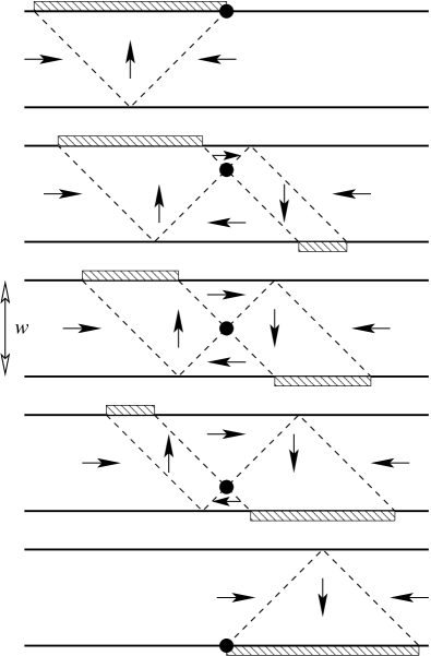
Figure 10: A very simple (4-Néel-wall) model of the vortex domain wall Chern (unpublished) The vortex core is denoted by the filled circle. Four Néel walls separate regions of uniform magnetization. Shaded areas indicate a buildup of magnetic charge. The panels show states with a fixed longitudinal coordinate of the vortex $X=\mathrm{const}$; the transverse coordinate is $Y=w/2$, $w/4$, 0, $-w/4$, and $-w/2$ respectively.

In this appendix we describe two models for the vortex domain wall based on two collective coordinates, the position of the vortex core $(X,Y)$. The simpler model provides a pedagogical introduction and the more sophisticated version is used to derive numerical values for the parameters used in Sec. IV.

In strips that support vortex domain walls, the dominant contribution to the energy in the absence of an applied field is due to magnetostatic interactions. For any domain wall in a strip of width $w$, thickness $t$, and saturation magnetization $M$, there is a total magnetic charge $Q=2\mu_{0}Mtw$ associated with the wall.Youk et al. (2006) In a vortex wall, nearly all of this charge is expelled to the edge of the strip. We thus focus on models in which there is no bound magnetic charge in the bulk of the strip.

We begin with a simple model in which a vortex wall consists of four straight Néel walls separating regions of uniform magnetization (Fig. 10). Two of these walls cross at the vortex core, and each edge defect has two walls emanating from it at $45^{\circ}$ angles from the edge. Despite its simplicity, the model captures some of the essential features of the vortex wall, including the chiral properties that lead to off-diagonal terms in the viscous tensor and the transverse component of the Zeeman force on the vortex.

Figure 11: 3-Néel-wall model of the vortex domain wall proposed in Ref. Youk et al., 2006. Solid lines denote straight Néel wall regions and dashed lines denote regions in which the Néel walls are parabolic.

While the 4-Néel-wall model described above correctly determines the form of the free energy and the sign of the off-diagonal viscosity term $\Gamma_{XY}$, it significantly overestimates the magnitude of the viscosity coefficients. This is mainly due to the inclusion of two Néel walls intersecting at the vortex core. In the more realistic model first proposed by Youk et al.Youk et al. (2006) one of these walls is replaced with two regions where magnetization rotates gradually (Fig. 11). In these curling regions, the magnetization angle is given by $\phi=\beta+\chi\pi/2$, where $\beta$ is the angular coordinate around the vortex core, originating at the $x$-axis, and $\chi=\pm 1$ is the chirality of the vortex. As a result, we are left with three Néel walls, with only one passing through the vortex. These walls are straight where they separate two uniform regions and parabolic where they separate a uniform and a curling region. This prevents bound magnetic charge in the bulk of the system.

We proceed in this appendix to derive the components of the viscosity tensor $\Gamma_{ij}$ and the values of the parameters $r$ and $k$ used in the energy (11). In each case we begin with a brief explanation using the simpler model before deriving the numerical values using the model of Youk et al.

C.1 Viscosity tensor

As long as the magnetization vector lies in the plane of the strip the definition of the viscosity tensor (6) may be expressed in terms of the azimuthal angle $\phi$ characterizing the magnetization:

$$\Gamma_{ij}=\alpha Jt\int d^{2}x\,\frac{\partial\phi}{\partial\xi_{i}}\frac{\partial\phi}{\partial\xi_{j}},$$ (60)

where $J=M/\gamma$ is the density of angular momentum and $t$ is the thickness of the film.

The largest contribution to the viscosity comes from regions where the magnetization angle depends strongly on the collective coordinates $X$ and $Y$. Note that the translational symmetry of the problem means that $\phi(x,X,y,Y)=\phi(x-X,y,Y)$, allowing us to make the replacement $\partial\phi/\partial X=-\partial\phi/\partial x$ in all cases, regardless of the model. In the simple model (Fig. 10) an infinitesimal shift in $X$ or $Y$ affects magnetization only in the vicinity of the Néel walls.

We begin by considering the contribution to the viscous tensor of the Néel walls that emanate from the vortex core at $\pm 45^{\circ}$. Near these walls, $\phi(x,y,X,Y)=f(x-X\mp y\pm Y)$. In these regions, derivatives with respect to collective coordinates may be reduced to ordinary gradients: $\partial\phi/\partial X=-\partial\phi/\partial x=-f^{\prime}$ and $\partial\phi/\partial Y=-\partial\phi/\partial y=\pm f^{\prime}$. As a result, the tensor components are equal to each other, up to a sign:

$$\Gamma_{XX}^{N}=\Gamma_{YY}^{N}=\mp\Gamma_{XY}^{N}=\alpha Jt\int d^{2}x\,{f^{\prime}}^{2}.$$ (61)

Opposite signs of the off-diagonal component $\Gamma_{XY}$ can be understood by noting that, as the vortex moves along $Y$, the two Néel walls that pass through it shift along $X$ in opposite directions, creating equal and opposite viscous forces in the $X$ direction.

As shown in Fig. 10, the two peripheral Néel walls move in the same direction as the central Néel wall perpendicular to them. Since they are also of the same length as that wall, they have the same contribution to the viscous tensor. Adding the contributions of all four Néel walls yields a total

$$\Gamma_{XX}=\Gamma_{YY}=2\chi\Gamma_{XY},$$ (62)

independent of the vortex position (for the simple model).

To obtain the absolute values, note that the expressions for viscosities (61) coincide, up to a constant factor, with the exchange energy of the Néel wall, which has been calculated, e.g., in Ref. Chern et al., 2006.

This energy may be determined by integrating the surface tension of the Néel wall, given by Chern et al. (2006)

$$\sigma=2A\int dv\left(\frac{\partial\phi}{\partial v}\right)^{2}=\frac{2\sqrt{2}A}{\lambda}\left(\sin{\phi_{0}}-\phi_{0}\cos\phi_{0}\right),$$ (63)

where $v$ is a coordinate perpendicular to the wall, and $2\phi_{0}$ is the angle of rotation across the wall. For a straight wall this angle is constant along the entire wall and the remaining integration along the wall is trivial. After an appropriate normalization we obtain viscosity coefficients

$$\Gamma_{XX}=\Gamma_{YY}=2\chi\Gamma_{XY}=0.608\alpha Jtw/\lambda$$ (64)

for the simple model, where the exchange length $\lambda=\sqrt{A/\mu_{0}M^{2}}=3.8$ nm in permalloy.

For a more accurate computation of the viscosity tensor, we turn to the model of Youk et al.Youk et al. (2006) (see Fig. 11). In this model, there are seven areas that contribute to the viscosity: 3 straight Néel wall segments, 2 parabolic Néel wall segments, and 2 regions of the bulk in which the magnetization curls.

Eq. (61) still holds for the straight Néel wall regions. However, one of the Néel walls passing through the vortex is now absent, and the outer walls have half the length of the inner. Their viscosity contribution is equal to that of the inner wall. As a result, the total contribution from the straight segments of Néel wall is

$$\Gamma^{S}_{XX}=\Gamma^{S}_{YY}=\chi\Gamma^{S}_{XY}=0.304\alpha Jtw/\lambda.$$ (65)

In a similar fashion, we may calculate the viscosity of the parabolic Néel wall segments. There is a slight complication in this case as these segments deform as the vortex moves across the strip.

The parabolic Néel walls in Fig. 11 are described by the equation $(x-X)^{2}=(2y\pm w)(2Y\pm w)$ for the upper and lower regions, respectively.Youk et al. (2006) Note that when the vortex moves straight up, the distance that a given point on the parabolic Néel wall moves is dependent on its $y$ coordinate. For an infinitesimal displacement $dY$ of the vortex upward from the center, a point on the parabolic Néel wall is moved to the left by $dY\sqrt{1\pm 2y/w}$. Thus, along these walls $\partial\phi/\partial Y=-(\partial\phi/\partial X)\sqrt{1\pm 2y/w}$.

In the case of the parabolic Néel walls, the angle $\phi_{0}$ changes along the length of the wall. For the lower wall, $\phi_{0}=(\arctan(y/\sqrt{w(w-2y)}))/2+\pi/4$. This is equal to the angle of the wall normal away from the $x$-axis. Therefore,

$$\int dx\left(\frac{\partial\phi}{\partial x}\right)^{2}=\frac{\sqrt{2}}{\lambda}(\sin{\phi_{0}}-\phi_{0}\cos\phi_{0})\cos\phi_{0}$$ (66)

in the region near the lower parabolic Néel wall. We assume that $\phi_{0}$ varies slowly on the scale of the Néel wall width. The variation of $\phi_{0}$ along the wall leads to parametrically small, width independent corrections to the Néel wall viscosity calculated here.

Making the usual replacement $\partial\phi/\partial X=-\partial\phi/\partial x$, we can perform the integration in Eq. (60) numerically for each tensor component. When the vortex is centered on the strip, the contribution of the parabolic walls to the viscosity is given by

$$\Gamma^{P}_{XX} = 0.057\alpha Jtw/\lambda,$$ (67a)

$$\Gamma^{P}_{YY} = 0.083\alpha Jtw/\lambda,$$ (67b)

$$\Gamma^{P}_{XY} = 0.069\alpha\chi Jtw/\lambda.$$ (67c)

The final contribution to the viscosity comes from those bulk regions in which the magnetization curls. In these regions, it is most convenient to carry out the integration of Eq. (60) in cylindrical coordinates $x-X=R\cos\beta$, $y-Y=R\sin\beta$. When the vortex is centered on the strip, we find

$$\Gamma_{ij} = \alpha Jt\int^{\beta_{0}}_{-\pi/2}d\beta\int^{-w/(2\sin\beta)}_{r_{0}}dR\,\frac{\partial\phi}{\partial\xi_{i}}\frac{\partial\phi}{\partial\xi_{j}}$$ (68)

$$+\alpha Jt\int^{0}_{\beta_{0}}d\beta\int^{w/(1+\sin\beta)}_{r_{0}}dR\,\frac{\partial\phi}{\partial\xi_{i}}\frac{\partial\phi}{\partial\xi_{j}},$$

where $\tan\beta_{0}=-1/\sqrt{8}$ and $r_{0}$ is the radius of the vortex core.

The magnetization in these regions is given simply by $\phi=\beta+\pi\chi/2$, so that $\partial\phi/\partial Y=-(\cos\beta)/R$, and $\partial\phi/\partial X=(\sin\beta)/R$. Integrating (68) numerically gives

$$\Gamma^{C}_{XX} = \alpha Jt\left(\frac{\pi}{4}\ln\frac{w}{r_{0}}-0.398\right),$$ (69a)

$$\Gamma^{C}_{YY} = \alpha Jt\left(\frac{\pi}{4}\ln\frac{w}{r_{0}}-0.010\right),$$ (69b)

$$\Gamma^{C}_{XY} = -\alpha\chi Jt\left(\frac{1}{2}\ln\frac{w}{r_{0}}-0.133\right).$$ (69c)

The symmetry of the domain wall when the vortex is centered on the strip implies that the contribution from both bulk curling regions is the same. Summing up all the contributions, we find

$$\!\!\!\!\Gamma_{XX} = \alpha Jt\left(0.418\frac{w}{\lambda}+\frac{\pi}{2}\ln\frac{w}{r_{0}}-0.797\right),$$ (70a)

$$\!\!\!\!\Gamma_{YY} = \alpha Jt\left(0.470\frac{w}{\lambda}+\frac{\pi}{2}\ln\frac{w}{r_{0}}-0.020\right),$$ (70b)

$$\!\!\!\!\Gamma_{XY} = \alpha\chi Jt\left(0.442\frac{w}{\lambda}-\ln\frac{w}{r_{0}}+0.265\right).$$ (70c)

It is instructive to compute the ratio of the viscous and gyrotropic forces $\Gamma_{ij}/G$ where $G=2\pi Jt$ is the gyrotropic constant. Taking the vortex core radius $r_{0}=\lambda=3.8$ nm, we obtain the dimensionless ratios listed in Table 1. The small value of Gilbert’s damping in permalloy, $\alpha\approx 0.01$, Freeman et al. (1998) leads to the dominance of the gyrotropic force in strips with submicron widths. The smallness of $\Gamma_{ij}/G$ can be exploited to organize an expansion in powers of this small parameter.

C.2 Free energy

In our simple model, magnetic charges form two lines of lengths $w-2Y$ and $w+2Y$ with constant charge density per unit length $\rho=\mu_{0}Mt$. As the vortex moves off-center, charge builds up on one edge of the strip or the other, leading to an increase in magnetostatic energy. The energy $E(Y)=E(0)+kY^{2}/2+\mathcal{O}(Y^{4})$ has a minimum at $Y=0$. (Here we chose $Y=0$ to be in the middle of the strip.) This leads to a force $-kY$ that acts to keep the vortex centered on the strip.

As can be seen from Fig. 10, transverse motion of the vortex core changes the total magnetization $M_{x}$ of the strip and thus affects its Zeeman energy. As the vortex core crosses from the top to the bottom edge of the strip, the Zeeman energy decreases linearly with the $y$-position of the core by a total of $4\mu_{0}HMtw^{2}$. The dependence of the energy of the magnetic configuration on the vortex core position $(X,Y)$ is therefore given by

$$U(X,Y)=-QH(X+2\chi Y)+E(Y).$$ (71)

The same principles hold true in the more realistic 3-Néel-wall model. As the vortex moves off center, the buildup of charge on one side of the strip causes a restoring force that pushes the vortex back toward the middle of the strip. As in 4-Néel-wall model, the Zeeman energy is given by $-QH(X+r\chi Y)$. Because the states of the system when the vortex is at either edge are the same as they are in the simplified model (see Figs. 10 and 11), the average value of $r$ as the vortex crosses the strip is again 2.

This is most likely an overestimate, as the states shown in Figs. 10 and 11 when the vortex is at an edge have an extended edge defect with a core radius equal to the width of the strip. In reality, the half-vortex core is less extended due to the exchange cost of the surrounding Néel walls. This smaller core for the edge defect means that the total charge on the wall moves less in the $X$ direction when the vortex crosses the strip than it does in either of the models listed here. This leads to a smaller value for $r$. By fitting the vortex trajectory in numerical simulations to that of our collective coordinate analysis, we found $r\approx 1.1$ in a strip with the width $w=200$ nm and thickness $t=20$ nm.

In what follows, we derive the energy of the vortex domain wall in the model proposed by Youk et al.Youk et al. (2006) to the second order in the displacement of the vortex from the center of the strip. As a result, we determine the value of the stiffness constant $k$. There are four contributions to the energy in this model: the Zeeman energy of the magnetization in the external field, the magnetostatic energy of the bound charges on the edges of the strip, the exchange energy of the bulk curling regions around the vortex, and the integrated Néel wall tension of the three Néel walls emanating from the topological defects.

If $(0,Y)$ is the position of the vortex, with $Y$ measured from the center of the strip, then the magnetization angles in the upper and lower curling regions are given by $\phi_{\pm}=\arctan((y-Y)/x)\mp\pi/2$. Thus there are charge densities $\rho_{\pm}(x)=\mu_{0}M\sin\phi_{\pm}(\mp w/2,x)=\mu_{0}M|x|/\sqrt{x^{2}+(w/2\mp Y)^{2}}$ spread out along the edges. The charge distributions are bounded in the center by the $X$ position of the vortex and outside by the points $L_{\pm}=\mp\sqrt{2w(w\pm 2Y)}$ at which the parabolic Néel wall segments hit the edges. The self-energies of these charged regions are given by

$$\frac{1}{8\pi\mu_{0}}\int_{0}^{t}\!\!dz\!\!\int_{0}^{t}\!\!dz^{\prime}\!\!\int_{0}^{L_{\pm}(Y)}\!\!\!\!\!\!\!\!\!\!\!\!dx\int_{0}^{L_{\pm}(Y)}\!\!\!\!\!\!\!\!\!\!\!\!dx^{\prime}\frac{\rho_{\pm}(x)\rho_{\pm}(x^{\prime})}{\sqrt{(x-x^{\prime})^{2}+(z-z^{\prime})^{2}}},$$

The interaction energy of the two charged segments is given by

$$\frac{1}{4\pi\mu_{0}}\int_{0}^{t}\!\!dz\!\!\int_{0}^{t}\!\!dz^{\prime}\!\!\int_{0}^{L_{+}(Y)}\!\!\!\!\!\!\!\!\!\!\!\!dx\int_{0}^{L_{-}(Y)}\!\!\!\!\!\!\!\!\!\!\!\!dx^{\prime}\frac{\rho_{+}(x)\rho_{-}(x^{\prime})}{\sqrt{(x+x^{\prime})^{2}+w^{2}+(z-z^{\prime})^{2}}}.$$

Expanding to the second order in $Y$ and integrating numerically, we find that the magnetostatic energy $E_{M}=E_{M}(0)+\frac{k_{M}}{2}Y^{2}$. The value of $k_{M}$ depends logarithmically on the aspect ratio $w/t$. For $w/t=10$, as in our numerical simulations,

$$k_{M}=1.08\frac{\mu_{0}M^{2}t^{2}}{w}.$$

In general,

$$k_{M}=f(w/t)\frac{\mu_{0}M^{2}t^{2}}{w},$$ (72)

where the value of $f$ is plotted in Fig. 12.

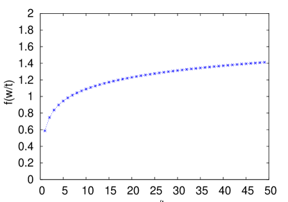
Figure 12: Value of the scaling function $f$ for various values of the aspect ratio $w/t$.

In addition, there is a significant contribution to the stiffness $k$ from the Néel walls. When the vortex is at the edge, the Néel wall energy is clearly lower than when it is at the center due to the absence of the parabolic segments. Note that there is no change in the energy of the straight Néel wall segments, because the total length and tension of these segments stay the same as the vortex moves.

The parabolic Néel walls are described by the equation $(x-X)^{2}=(2y\pm w)(2Y\pm w)$ for the upper and lower regions, respectively. By symmetry, the total energy of the upper parabolic segment, when the vortex position is $(X,Y)$, will be the same as that of the lower parabolic segment when the vortex position is $(X,-Y)$. Thus, the contribution of each parabolic segment to the stiffness constant will be the same. We shall restrict our consideration to the lower wall for simplicity.

It is convenient to derive the energy of the parabolic Néel wall by switching to cylindrical coordinates around the vortex core. Namely, $R=\sqrt{(x-X)^{2}+(y-Y)^{2}}$ and $\beta=\arctan((y-Y)/(x-X))$. In these coordinates, the lower parabolic wall is given by $R=(w-2Y)/(1+\sin\beta)$.

The surface tension of a Néel wall is given by Eq. (63), where $\lambda=\sqrt{A/\mu_{0}M^{2}}$. In the case of the parabolic Néel walls, the rotation angle $\phi_{0}$ is equal to the angle of the wall normal away from the $x$-axis. This wall normal changes with $\beta$. For the lower wall, $\phi_{0}=\beta/2+\pi/4$. The wall hits the edge of the strip when $\beta=\beta_{0}(Y)=-\arcsin((w+2Y)/(3w-2Y))$.

The line element along the parabolic segment is given by $dl=\sqrt{dr^{2}+r^{2}d\beta^{2}}=(w-2y)d\beta\csc\phi_{0}/(1+\sin\beta)$. Hence, the energy of the lower parabolic Néel wall is

$$E_{p-}=2\sqrt{2}\mu_{0}M^{2}\lambda t(w-2Y)\int^{0}_{\beta_{0}(Y)}\!\!\!d\beta\,\frac{1-\phi_{0}(\beta)\cot\phi_{0}(\beta)}{1+\sin\beta}.$$ (73)

Taking the second derivative of this energy with respect to $Y$ at $Y=0$ yields the contribution

$$\frac{k_{p}}{2}=-\frac{4\mu_{0}M^{2}\lambda t}{3w}$$ (74)

of the parabolic Néel walls to the spring constant $k$, where the factor of $2$ on the left hand side comes from the inclusion of the upper parabolic wall as well as the lower.

Finally, there is a smaller contribution to the stiffness $k$ from the bulk regions of nonuniform magnetization. Again, the symmetry of the problem allows us to focus on the lower region and simply double our result to find the total contribution. Using the cylindrical coordinates and definition of $\beta_{0}$, we find that the exchange energy of the lower region is given by

$$E_{\mathrm{ex-}} = \mu_{0}M^{2}t\int d^{2}x\,\frac{\lambda^{2}}{r^{2}}$$

$$= \mu_{0}M^{2}\lambda^{2}t\int^{\beta_{0}(Y)}_{-\pi/2}d\beta\ln\frac{-(w+2Y)}{2r_{0}\sin\beta}$$

$$+\mu_{0}M^{2}\lambda^{2}t\int^{0}_{\beta_{0}}d\beta\ln\frac{(w-2Y)}{r_{0}(1+\sin\beta)},$$

where $r_{0}$ is the radius of the vortex core. If we again take the second derivative with respect to $Y$ at $Y=0$, we obtain

$$\frac{k_{\mathrm{ex}}}{2}=-\left(\pi+\frac{4\sqrt{2}}{9}\right)\frac{2\mu_{0}M^{2}\lambda^{2}t}{w^{2}}.$$ (75)

In total, we find that

$$k = k_{M}+k_{p}+k_{\mathrm{ex}}$$

$$\approx \left[f(w/t)-\frac{8\lambda}{3t}-\frac{4\lambda^{2}}{tw}\left(\pi+\frac{4\sqrt{2}}{9}\right)\right]\frac{\mu_{0}M^{2}t^{2}}{w}.$$

For $t=20$ nm, $\lambda=3.8$ nm, and $w=200$ nm, this gives

$$k=0.49\frac{\mu_{0}M^{2}t^{2}}{w}.$$ (77)

References

- Allwood et al. (2005) D. A. Allwood, G. Xiong, C. C. Faulkner, D. Atkinson, D. Petit, and R. P. Cowburn, Science 309, 1688 (2005).
- Thomas et al. (2007) L. Thomas, M. Hayashi, X. Jiang, R. Moriya, C. Rettner, and S. Parkin, Science 315, 1553 (2007).
- Chien et al. (June 2007) C. L. Chien, F. Q. Zhu, and J. G. Zhu, Physics Today 60, 40 (June 2007).
- Beach et al. (2005) G. S. D. Beach, C. Nistor, C. Knutson, M. Tsoi, and J. L. Erskine, Nature Mat. 4, 741 (2005).
- Tchernyshyov and Chern (2005) O. Tchernyshyov and G.-W. Chern, Phys. Rev. Lett. 95, 197204 (2005).
- Tretiakov et al. (2008) O. A. Tretiakov, D. Clarke, G.-W. Chern, Y. B. Bazaliy, and O. Tchernyshyov, Phys. Rev. Lett. 100, 127204 (2008).
- Gilbert (1955) T. L. Gilbert, Phys. Rev. 100, 1243 (1955).
- Gilbert (2004) T. L. Gilbert, IEEE Trans. Mag. 40, 3443 (2004).
- Donahue and Porter (1999) M. J. Donahue and D. G. Porter, Tech. Rep. NISTIR 6376, National Institute of Standards and Technology, Gaithersburg, MD (1999), http://math.nist.gov/oommf.
- McMichael and Donahue (1997) R. D. McMichael and M. J. Donahue, IEEE Trans. Magn. 33, 4167 (1997).
- Youk et al. (2006) H. Youk, G.-W. Chern, K. Merit, B. Oppenheimer, and O. Tchernyshyov, J. Appl. Phys. 99, 08B101 (2006).
- Freeman et al. (1998) M. R. Freeman, W. K. Hiebert, and A. Stankiewicz, J. Appl. Phys. 83, 6217 (1998).
- Schryer and Walker (1974) N. L. Schryer and L. R. Walker, J. Appl. Phys. 45, 5406 (1974).
- Thiaville and Nakatani (2006) A. Thiaville and Y. Nakatani, in Spin Dynamics in Confined Magnetic Structures III (Springer, 2006), vol. 101 of Topics in applied physics, pp. 161–205.
- Hayashi et al. (2007) M. Hayashi, L. Thomas, C. Rettner, R. Moriya, and S. S. P. Parkin, Nat. Phys. 3, 21 (2007).
- Lee et al. (2007) J.-Y. Lee, K.-S. Lee, S. Choi, K. Y. Guslienko, and S.-K. Kim, Phys. Rev. B 76, 184408 (2007).
- Guslienko et al. (unpublished) K. Y. Guslienko, J.-Y. Lee, and S.-K. Kim (unpublished), eprint arXiv:0711.3680v1.
- Saitoh et al. (2004) E. Saitoh, H. Miyajima, T. Yamaoka, and G. Tatara, Nature 432, 203 (2004).
- Döring (1948) V. W. Döring, Z. Naturforsch 3a, 373 (1948).
- Tatara and Kohno (2004) G. Tatara and H. Kohno, Phys. Rev. Lett. 92, 086601 (2004).
- Yang et al. (2008) J. Yang, C. Nistor, G. S. D. Beach, and J. L. Erskine, Phys. Rev. B. 77, 014413 (2008).
- Wachowiak et al. (2002) A. Wachowiak, J. Wiebe, M. Bode, O. Pietzsch, M. Morgenstern, and R. Wiesendanger, Science 298, 577 (2002).
- Guslienko et al. (2008) K. Y. Guslienko, K.-S. Lee, and S.-K. Kim, Phys. Rev. Lett. 100, 027203 (2008).
- Van Waeyenberge et al. (2006) B. Van Waeyenberge, A. Puzic, H. Stoll, K. W. Chou, T. Tyliszczak, R. Hertel, M. Fahnle, H. Brückl, K. Rott, G. Reiss, et al., Nature (London) 444, 461 (2006).
- Komineas (2007) S. Komineas, Phys. Rev. Lett. 99, 117202 (2007).
- Hertel and Schneider (2006) R. Hertel and C. M. Schneider, Phys. Rev. Lett. 97, 177202 (2006).
- Tretiakov and Tchernyshyov (2007) O. A. Tretiakov and O. Tchernyshyov, Phys. Rev. B 75, 012408 (2007).
- Belavin and Polyakov (1975) A. A. Belavin and A. M. Polyakov, Pis’ma ZheETF 22, 503 (1975), [JETP Lett. 22, 245 (1975)].
- Chern (unpublished) G.-W. Chern (unpublished).
- Chern et al. (2006) G.-W. Chern, H. Youk, and O. Tchernyshyov, J. Appl. Phys. 99, 08Q505 (2006).