An Integrated Picture of Star Formation, Metallicity Evolution, and Galactic Stellar Mass Assembly

Abstract

We present an integrated study of star formation and galactic stellar mass assembly from $z=0.05-1.5$ and galactic metallicity evolution from $z=0.05-0.9$ using a very large and highly spectroscopically complete sample selected by rest-frame NIR bolometric flux. Our NIR (rest-frame $0.8-2.4~{}\mu$m) sample consists of 2634 galaxies with fluxes in excess of $2\times 10^{-15}$ ergs cm${}^{-2}$ s${}^{-1}$ in the GOODS-N field. It probes to a complete mass limit of $10^{10}$ M${}_{\odot}$ for $z=0.05-0.9$ and includes all Milky Way mass galaxies for $z=0.05-1.5$. We have spectroscopic redshifts and high-quality spectra from $4500-10000$ Å for 2020 (77%) of the galaxies. Our 13-band photometric redshift estimates show that most of the spectroscopically unidentified sources in the above redshift ranges are early-type galaxies. We assume a Salpeter IMF and fit Bruzual & Charlot (2003) models to the data to compute the galactic stellar masses and extinctions. We calibrate the star formation diagnostics internally using our $z=0.05-0.475$ sample. We then derive the galactic stellar mass assembly and star formation histories. We compare our extinction corrected UV-based star formation rate densities with the combination of the star formation rate densities that we compute from the 24 $\mu$m fluxes and the extinction uncorrected [O$\thinspace{\rm II}]$ luminosities. We determine the expected formed stellar mass density growth rates produced by star formation and compare them with the growth rates measured from the formed stellar mass functions by mass interval. We show that the growth rates match if the IMF is slightly increased from the Salpeter IMF at intermediate masses ($\sim 10$ M${}_{\odot}$). We investigate the evolution of galaxy color, spectral type, and morphology with mass and redshift and the evolution of mass with environment. We find that applying extinction corrections is critical when analyzing the galaxy colors. As an example, prior to correcting for extinction, nearly all of the galaxies in the green valley are 24 $\mu$m sources, but after correcting for extinction, the bulk of the 24 $\mu$m sources lie in the blue cloud. We also compute the metallicities of the sources between $z=0.05-0.9$ that have well-detected H$\beta$, [O$\thinspace{\rm II}]$ $\lambda 3727$, and [O$\thinspace{\rm III}]$ $\lambda 5007$ emission lines using the R23 diagnostic ratio. At $z<0.475$ we use the R23, [N$\thinspace{\rm II}]$/[O$\thinspace{\rm II}]$, and [N$\thinspace{\rm II}]$/H$\alpha$ diagnostic ratios. We find an evolution of the metallicity-mass relation corresponding to a decrease of $0.21\pm 0.03$ dex between the local value and the value at $z=0.77$ in the $10^{10}-10^{11}$ M${}_{\odot}$ range. We use the metallicity evolution to estimate the gas mass of the galaxies, which we compare with the galactic stellar mass assembly and star formation histories. Overall, our measurements are consistent with a galaxy evolution process dominated by episodic bursts of star formation and where star formation in the most massive galaxies ($\gtrsim 10^{11}$ M${}_{\odot}$) ceases at $z<1.5$ because of gas starvation.

1. Introduction

One of the fundamental goals of modern cosmology is to understand the formation and evolution of the galaxy population as a whole. We shall refer to this as the cosmic galaxy formation problem. There has been spectacular progress in addressing the cosmic galaxy formation problem over the last twenty years, beginning with the determination of the star formation history (e.g., Cowie et al. 1995; Lilly et al. 1996; Madau et al. 1996; Steidel et al. 1999; Haarsma et al. 2000; Barger et al. 2000; Le Floc’h et al. 2005; Pérez-González et al. 2005; Hopkins & Beacom 2006; Wang et al. 2006; Reddy et al. 2008). This has been followed more recently by efforts to measure the galactic stellar mass assembly history (e.g., Brinchmann & Ellis 2000; Cole et al. 2001; Bell et al. 2003, 2007; Pérez-González et al. 2003, 2008; Dickinson et al. 2003; Rudnick et al. 2003, 2006; Fontana et al. 2003, 2004, 2006; Drory et al. 2004, 2005; Bundy et al. 2005, 2006; Conselice et al. 2005, 2007; Borch et al. 2006; Pannella et al. 2006; Elsner et al. 2008) and the evolution of metallicity with galaxy mass and redshift (e.g., Kobulnicky et al. 2003; Lilly et al. 2003; Kobulnicky & Kewley 2004; Tremonti et al. 2004; Liang et al. 2004; Savaglio et al. 2005). However, ideally what one wants is a comprehensive analysis of the history of star formation, the growth of galactic stellar mass and metals content, and the changes in morphology with redshift, galaxy mass, and the environment for a large, mass-selected galaxy sample that could be compared in detail with local galaxy properties and cosmological simulations of galaxy evolution. In particular, such an analysis could yield clear explanations for the migration of star formation to lower mass galaxies at later cosmic times and the simultaneous quenching of star formation in the most massive galaxies (the downsizing of Cowie et al. 1996), as well as for the color bimodality of galaxy populations (e.g., Strateva et al. 2001; Baldry et al. 2004).

Up until now such an analysis has not been possible since existing data sets are either visually selected, have limited color information, and are poorly suited to a metals analysis because of the spectroscopic wavelength coverage (e.g., the DEEP2 survey); mass selected but based on photometric redshifts (e.g., Combo17/GEMS); or mass selected and spectroscopically observed but based on a relatively small sample (e.g., the Gemini Deep Deep Survey).

In this paper we present, for the first time, an integrated, mass-based analysis made possible by the availability of a large, homogeneous, near-infrared (NIR) selected and spectroscopically observed galaxy sample in the Great Observatories Origins Deep Survey-North (GOODS-N; Giavalisco et al. 2004) field. We have obtained extremely deep, wide-field NIR images (Keenan et al. 2008, in preparation) and highly complete spectroscopic identifications of the sources in this field (Barger et al. 2008, in preparation). We are therefore able to use, for the most part, spectroscopic redshifts to make our determinations of the galactic stellar mass assembly and star formation histories, as well as high-quality measurements of line fluxes to obtain the metallicity history.

However, we caution that even with such an excellent data set there are many complicating factors in relating the star formation history to the stellar mass assembly history and the formation of metals in galaxies, even at late cosmic times. (Here we shall take late cosmic times to be $z<1.5$.) At the conceptual level, methods of measuring star formation rates use diagnostics which are sensitive to the high-mass end of the stellar initial mass function (IMF), while stellar mass measurements are dominated by lower mass stars. Therefore, while the shape of the sub-solar IMF only enters as a normalization factor, the shape of the IMF at higher masses is critical in relating the star formation rates to the stellar masses. Thus, we must be concerned about the uncertainties in the IMF shape and the potential variations in the IMF shape between different types of galaxies. In principle we could minimize this problem by considering the growth of the stellar mass in metals rather than the growth of the total stellar mass, since the metals are produced by the same high-mass stars that are measured by the star formation diagnostics (Cowie 1988). However, even this is subject to uncertainties in the yields and would require the measurement of not only the total stellar mass evolution but also the metals evolution in both stars and gas, which would be very challenging to do.

Measurements of the star formation rates, stellar masses, and metals are also complicated by other factors. Extinction reradiates light from the rest-frame UV to the far-infrared (FIR), and we must determine total star formation rates over a wide range of galaxies with radically different morphologies and dust column densities. Conversions even of NIR light to stellar mass are complicated by ongoing active star formation, and there are still major uncertainties in the stellar modeling of the galaxy populations. Finally, determinations of the metals throughout the redshift range of interest can only be made for the gaseous baryons in the star-forming galaxies and depend on the notoriously uncertain conversions of the strong oxygen and nitrogen emission lines to metallicities.

Cosmic variance is also a significant issue in a field size as small as the GOODS-N (e.g. Somerville et al. 2004) and can affect our analysis of the evolution of quantities such as the galaxy mass density and the universal star formation rates.

These problems must be borne in mind throughout any work of the present type, and we attempt at all points to work forward as self-consistently as possible from the raw information (NIR luminosities, galaxy line strengths, raw star formation diagnostics, etc.) to inferences about the evolution of derived quantities, such as stellar masses, star formation rates, and metallicities. Also, wherever possible, we have used multiple independent methods to determine the sensitivity of the derived quantities to our underlying assumptions. We attempt to self consistently estimate the effects of cosmic variance within the data set and also to estimate the effects which analytic error estimates of the variance could introduce in our analysis. Finally we compare our results throughout to other recent work using different, and in some cases much larger, fields to check for consistency in these portions of the paper.

The outline of the paper is as follows. In §2 and §3 we describe the basic data and the sample selections. In §4 we fit Bruzual & Charlot (2003) models to the data to determine galactic stellar masses and extinctions in the galaxies. In §5 we measure equivalent widths and line fluxes from the spectra. In §6 we compare measurements of the continuum and line extinctions. In §7 we derive self-consistent calibrations of the various star formation rate diagnostics. In §8 and §9 we derive the metallicities with mass and redshift using various metallicity diagnostics. In §LABEL:secabs we consider the galaxies missing from the metals analysis. This is a long paper, and some readers may wish to skip much of the detail and move to the discussion (§LABEL:secdisc) and summary (§LABEL:seccon), which we have tried to make separately readable and which contain the high-level interpretation of the data, including the derivation of the stellar mass assembly history with redshift, the evolution of the mass-metallicity and mass-morphology relations with redshift and environment, and the use of the metals evolution to derive an estimate of the baryonic gas mass reservoir in the galaxies. We find that all of our measurements provide a broad, self-consistent picture of a galaxy evolution process dominated by episodic bursts of star formation and where star formation in the most massive galaxies is terminated at later cosmic times as a consequence of gas starvation.

We adopt the $-1.35$ power-law Salpeter IMF (Salpeter 1955) extending from 0.1 to 100 M${}_{\odot}$ for ease of comparison with previous results. Most importantly, this allows us to compare directly with the local mass function computed by Cole et al. (2001; hereafter, Cole01) for this IMF. The Salpeter IMF only differs significantly from the current best IMFs (Kroupa 2001; Chabrier 2003) below 1 M${}_{\odot}$, and thus these three IMFs differ only in the normalization of the galactic stellar mass and star formation rate determinations. We can convert the total mass formed into stars prior to stellar mass loss (which we will refer to as the formed stellar mass to distinguish it from the present stellar mass, which is the stellar mass present at any given time) from the Salpeter IMF to the Chabrier IMF by dividing by 1.39 and to the Kroupa IMF by dividing by 1.31. The exact conversion when considering the present stellar masses rather than the formed stellar masses depends on the average evolutionary stage of the galaxies. However, this dependence is relatively weak, and we may approximately convert the present stellar mass from the Salpeter IMF to the Chabrier IMF by dividing by 1.70 and to the Kroupa IMF by dividing by 1.54. Note that these latter conversion factors have been computed for the distribution of ages in our ensemble of galaxies. The present stellar mass for the Salpeter IMF is roughly 0.74 of the formed stellar mass.

We assume $\Omega_{M}=0.3$, $\Omega_{\Lambda}=0.7$, and $H_{0}=70$ km s${}^{-1}$ Mpc${}^{-1}$ throughout. All magnitudes are given in the AB magnitude system, where an AB magnitude is defined by $m_{AB}=-2.5\log f_{\nu}-48.60$. Here $f_{\nu}$ is the flux of the source in units of ergs cm${}^{-2}$ s${}^{-1}$ Hz${}^{-1}$. We assume a reference value of the solar metallicity of $12+\log({\rm O/H})=8.66$ and a conversion to the mass fraction of metals of $Z=0.0126$ (Asplund et al. 2004). This conversion is weakly dependent on the assumed chemical composition relative to the oxygen abundance.

The observed area in the GOODS-N. The area is centered on RA(2000) and Dec(2000) coordinates (189.2282, 62.2375) with corners at (189.5435, 62.2749), (188.9137, 62.2000), (189.3090, 62.3824), and (189.1482, 62.0909). The covered area is 145 arcmin${}^{2}$ ($9\farcm 3$ by $15\farcm 7$). The NIR-selected sample is shown with black dots, the 663 24 $\mu$m detected sources with red squares, the 229 X-ray detected sources with blue diamonds, and the 97 20 cm detected sources with green open triangles. The concentration of the X-ray sources to the field center reflects the variation in the sensitivity of the X-ray image over the field.

2. The NIR Bolometric Flux Sample

2.1. Photometric Selection

The GOODS-N field is one of the most intensively studied regions in the sky, and in many bandpasses it has the deepest images ever obtained. Thus, it is nearly ideal for the present study. In this paper we use photometric data taken from existing work. The optical magnitudes are from the Subaru 8.2 m SuprimeCam observations of Capak et al. (2004; $U,B,V,R,I,z^{\prime}$) and from the HST Advanced Camera for Surveys (ACS) observations of Giavalisco et al. (2004; F435W, F606W, F775W, and F850LP). The NIR magnitudes are from the University of Hawaii 2.2 m ULBCAM ($J,H$) and CFHT WIRCAM and Subaru 8.2 m MOIRCS ($K_{s}$) observations of Keenan et al. (2008, in preparation). To properly match to the optical data, the $3.6,4.5,5.8$, and $8.0~{}\mu$m magnitudes were measured directly from the IRAC images that Wang et al. (2006) produced. Weighting by exposure time, Wang et al. (2006) combined the reduced DR1 and DR2 IRAC superdeep images from the Spitzer Legacy first, interim, and second data release products (DR1, DR1+, DR2; Dickinson et al. 2008, in preparation). In all cases, only sources within the well-covered ACS GOODS-N region were included, as summarized in Figure 1. The covered area is 145 arcmin${}^{2}$.

For all of the sources we used corrected aperture magnitudes to compute the colors and spectral energy distributions (SEDs). We used $3^{\prime\prime}$ diameter apertures for the optical and NIR data and $6^{\prime\prime}$ diameter apertures for the MIR data. We computed the median of the difference between these magnitudes and aperture magnitudes computed in $6^{\prime\prime}$ diameter apertures for the the optical and $12^{\prime\prime}$ diameter apertures for the MIR data and used this median to correct the smaller aperture magnitude to an approximate total magnitude. For the brighter extended sources we also computed isophotal magnitudes integrated to 0.01% of the peak surface brightness and used the difference between these and the corrected aperture magnitudes in the $K_{s}$ band to correct the luminosities and masses. All of the calibrations are independent, so it is important to check that we have fully consistent magnitudes. We will return to this point in §5.1.

We computed a rest-frame NIR bolometric flux for all of the sources in the region which were significantly detected at any of the observed wavelength bands by linearly interpolating the observed mangitudes to form a rest frame SED. We used spectroscopic redshifts, where these were known, or otherwise photometric redshifts, which we calculated as in Wang et al. (2006) using the template method developed by Pérez-González et al. (2005). We computed the flux over the rest-frame wavelength range 8000 Å to $2.4~{}\mu$m. We excluded from the sample the spectroscopically identified stars and all of the sources within $3^{\prime\prime}$ of a brighter object or within $12^{\prime\prime}$ of the eleven brightest stars, leaving a final sample of 2634 galaxies with fluxes above $2\times 10^{-15}$ ergs cm${}^{-2}$ s${}^{-1}$. We take this as our primary NIR sample. Our exclusion of neighbor sources introduces a small, flux-dependent correction to the area, which we allow for in our determinations of the mass functions, but the correction never exceeds 10%, even at the faintest fluxes.

Our selection by rest frame NIR bolometric flux is compared with the more usual selection by observed NIR magnitude ($K_{s,{\rm AB}}$) in Figure 2.1 for sources with $z=0.05-1.5$. The best-fit relation gives

$$K_{s,{\rm AB}}=-11.87-2.40\log({\rm NIR~{}flux})\,,$$ (1)

and the limiting NIR flux corresponds roughly to $K_{s,{\rm AB}}=23.4$. This is a shallow sample compared to the depth of the NIR images. For the $K_{s}$ image it corresponds to an $18\sigma$ selection. Thus, there should be no significant selection biases.

Comparison of the rest-frame NIR bolometric flux with the observed $K_{s}$ magnitude for sources with $z=0.05-1.5$. The red diagonal line shows the least-square polynomial fit of $\log$(NIR flux) to $K_{s}$ magnitude. The blue dashed horizontal line shows the $5\sigma$ flux limit of $24.8$ for the $K_{s}$ sample.

We identified X-ray counterparts to the NIR sample by matching our sample to the sources detected in the Alexander et al. (2003) catalog of the 2 Ms Chandra Deep Field-North (CDF-N) using a $2^{\prime\prime}$ search radius. Near the aim point the CDF-N X-ray data reach limiting fluxes of $\approx 1.5\times 10^{-17}$ ($0.5-2$ keV) and $\approx 1.4\times 10^{-16}$ ergs cm${}^{-2}$ s${}^{-1}$ ($2-8$ keV). We similarly obtained the radio fluxes from the Richards (2000) 1.4 GHz catalog, which reaches a $5\sigma$ limiting flux of $40~{}\mu$Jy and the $24~{}\mu$m fluxes are from the DR1+ MIPS $24~{}\mu$m source list and version 0.36 MIPS $24~{}\mu$m map provided by the Spitzer Legacy Program. This source catalog is flux-limited at $80~{}\mu$Jy and is a subset of a more extensive catalog (R. R. Chary et al. 2007, in preparation).

Our NIR-selected sample, together with the X-ray, 20 cm, and $24~{}\mu$m detected sources, are shown in Figure 1.

2.2. Spectroscopy

Following the establishment of the Hubble Deep Field-North (HDF-N) with HST, intensive spectroscopic observations of the region were made by a number of groups, primarily using the Low-Resolution Imaging Spectrograph (LRIS; Oke et al. 1995) on the Keck I 10 m telescope (these data are summarized in Cohen et al. 2000). After the more extended GOODS-N region was observed with the ACS camera, a number of groups began intensive spectroscopic observations with the large-format Deep Extragalactic Imaging Multi-Object Spectrograph (DEIMOS; Faber et al. 2003) on the Keck II 10 m telescope. Wirth et al. (2004; Keck Team Redshift Survey or KTRS) and Cowie et al. (2004) presented large samples of magnitude-selected redshifts, while Reddy et al. (2006) gave a substantial sample of $z=2-3$ color-selected redshifts, Chapman et al. (2004, 2005) and Swinbank et al. (2004) presented a number of radio/submillimeter redshifts, Treu et al. (2005) measured redshifts for a sample of spheroids, and Barger et al. (2005, 2007) carried out observations on the X-ray and 1.4 GHz samples.

We have attempted to make the most complete and homogeneous spectral database possible by observing all of the missing or unidentified galaxies in a variety of flux-limited samples. A more extensive description of these samples may be found in Barger et al. (2007, in preparation). In this paper we focus only on the spectroscopic observations of our NIR sample. Our observations were made in a number of DEIMOS runs between 2004 and 2007. We used the 600 lines per mm grating, giving a resolution of $3.5$ Å and a wavelength coverage of $5300$ Å, which was the configuration used in the KTRS and in the Cowie et al. (2004) observations. The spectra were centered at an average wavelength of $7200$ Å, though the exact wavelength range for each spectrum depends on the slit position. Each $\sim 1$ hr exposure was broken into three subsets, with the objects stepped along the slit by $1.5^{\prime\prime}$ in each direction. Unidentified objects were continuously reobserved, giving maximum exposure times of up to 7 hrs. The spectra were reduced in the same way as previous LRIS spectra (Cowie et al. 1996). The dithering procedure provides extremely high-precision sky subtraction, which is important if we wish to measure accurate equivalent widths, as in the present paper. We have only included spectra in the sample that could be confidently identified based on multiple emission and/or absorption lines.

We also reobserved objects where the original spectra were of poor quality or where previous redshifts were obtained with instruments other than DEIMOS, as well as where the existing redshift identifications were unconvincing or where there were conflicting redshifts in the literature (a small number of sources). Many of the KTRS spectra have poor sky subtraction. While these spectra are adequate for redshift identifications, they are not suitable for line measurements because of the residual sky lines. For the fainter objects the absolute sky subtraction is often problematic and, in some cases, the spectra even have negative continua. Equivalent width measurements made on such spectra have very large systematic uncertainties. This is a substantial problem for previous work (e.g., Kobulnicky & Kewley 2004) that relied on the KTRS spectra. We have reobserved most of these sources.

We now have spectroscopic redshift identifications for 2020 of the 2634 galaxies (77%) in our NIR sample. We show the redshift distribution for the spectroscopically identified sample in Figure 2.2 (black histogram). The photometric redshift analysis of the remaining sources (red histogram) implies that most of these sources lie outside of our redshift ranges of interest ($z=0.05-0.9$ for our metallicity analysis and $z=0.05-1.5$ for our mass assembly and star formation analyses) and hence that the spectroscopic completeness inside our two redshift ranges of interest is extremely high.

We assigned photometric redshifts to all but 14 of the sources in our sample. These 14 sources are either extremely faint or have peculiar SEDs that could not be adequately fitted by the templates. We shall assume that these lie outside of our redshift ranges of interest. Between $z=0$ and $z=0.9$ there are 1260 spectroscopically identified sources, and between $z=0$ and $z=1.5$ there are 1884 spectroscopically identified sources. Photometric redshifts add a further 126 sources to $z=0.05-0.9$ and a further 229 sources to $z=0.9-1.5$. Based on the SEDs of the sources with only photometric redshifts in these ranges, many are red galaxies, which are more difficult to identify spectroscopically. Of the bluer sources, some may have photometric redshifts that have scattered into these redshift ranges, even though their true redshifts are higher. Of the 126 galaxies with only photometric redshifts in the redshift range $z=0.05-0.9$, 87 have been spectroscopically observed and none of these have strong emission lines. Emission lines, if present, would have easily been observed in this redshift range.

Redshift distribution of our full NIR sample. Black (red) histogram shows spectroscopic (photometric) redshifts. The redshift bin size is 0.01.

We conclude that the spectroscopic sample contains nearly all of the sources (1260 out of a maximum of 1386, or $>91$%) lying in the redshift range $z=0.05-0.9$ and essentially all of the sources with strong emission lines suitable for measuring emission line metallicities in this redshift range. Over the $z=0.05-1.5$ interval the spectroscopically identified sample contains $>84$% of the galaxies (1884 out of a maximum of 2239).

2.3. Galaxy Morphologies

The galaxy morphological types are taken from Bundy et al. (2005) wherever possible. The Bundy et al. catalog is based on Richard Ellis’s visual classification of the sources in the GOODS-N according to the following scale: $-2=$ Star, $-1=$ Compact, $0=$ E, $1=$ E/S0, $2=$ S0, $3=$ Sab, $4=$ S, $5=$ Scd, $6=$ Irr, $7=$ Unclass, $8=$ Merger, and $9=$ Fault. For galaxies in our sample which were not included in the Bundy et al. (2005) catalog, we visually classified the sources using the HST F850LP images, aiming to reproduce the Ellis classifications as closely as possible.

2.4. Galaxy Environments

The local galaxy density can be computed using the distance to the $n$th nearest neighbor (Dressler 1980). In the present work we use the velocity information only to separate slices; otherwise we use the projected distance $d_{n}$. The surface density is then given by $\Sigma=n/(\pi d_{n}^{2})$. An extensive comparison of this measure of the density environment with other methods is given in Cooper et al. (2005), who conclude that the projected distance method is generally the most robust for this type of work.

Edge effects are important in small field areas, such as the GOODS-N region, and can bias the density parameter in low density regions where the projected separation extends beyond the edge of the field. We correct for this effect by including only that part of the area $\pi d_{n}^{2}$ which lies within the field (e.g., Baldry et al. 2006). To further reduce the edge effects, we use a low $n$ to minimize the projected distance and also exclude regions of the field that, at the redshift of the galaxy, lie too close to the edge of the field for an accurate measurement.

Thus, for each galaxy we computed the projected density based on the 3rd nearest neighbor having a mass above a uniform mass cut and lying within 1000 km s${}^{-1}$ of the galaxy. We exclude galaxies which lie closer than 1 Mpc from the sample edge. This constraint restricts to galaxies with $z\gtrsim 0.3$, since all of the lower redshift galaxies will lie too close to the edges of the field.

3. Four Uniform NIR Luminosity Samples

(a) NIR luminosity vs. spectroscopic redshift for the spectroscopically identified sources in the NIR sample, and (b) NIR luminosity vs. photometric redshift for the spectroscopically unidentified sources in the NIR sample. The blue solid squares show sources with blue spectra, where massive stars may still make a substantial contribution to the NIR luminosity. The red open diamonds show sources containing AGNs based on their X-ray luminosities. The red solid curve shows the luminosity corresponding to the limiting NIR flux of $2\times 10^{-15}$ ergs cm${}^{-2}$ s${}^{-1}$. The red (black) dashed lines mark the region that corresponds to the mid-$z$ (low-$z$) uniform NIR luminosity sample, where the [O$\thinspace{\rm III}]$ $\lambda 5007$ (H$\alpha$) line would be in the spectrum.

In Figure 3a (3b) we show NIR luminosity versus spectroscopic (photometric) redshift for the spectroscopically identified (unidentified) NIR sample. We denote sources with blue spectra, where massive stars may still make a substantial contribution to the NIR luminosity, by blue solid squares. We denote sources that contain AGNs (based on whether either their $2-8$ keV or $0.5-2$ keV luminosities are $>10^{42}$ ergs s${}^{-1}$) by red open diamonds. We show the luminosity corresponding to the limiting NIR flux of $2\times 10^{-15}$ ergs cm${}^{-2}$ s${}^{-1}$ by the solid red curve.

NIR luminosity vs. redshift for the spectroscopically identified sources in the (a) mid-$z$ sample and (b) low-$z$ sample. The sources with emission (absorption) line redshifts are denoted by black squares (red diamonds).

We construct two uniform NIR luminosity samples for our metallicity analysis: a mid-$z$ sample and a low-$z$ sample. Although most of the spectra extend to about $1~{}\mu$m, the sensitivity falls rapidly at the reddest wavelengths, and some spectra are cut off at wavelengths $<1~{}\mu$m because of their mask positions. Thus, we choose a limiting upper wavelength of 9500 Å. The limiting upper wavelength of 9500 Å corresponds to $z<0.9$ ($z<0.475$) for the [O$\thinspace{\rm III}]$ $\lambda$5007 Å (H$\alpha$) line to be observable if present. In each case this sets a lower limit on the NIR luminosity, which corresponds to the NIR flux limit at the maximum redshift. The mid-$z$ sample has $z=0.05-0.9$ and NIR luminosity $>8\times 10^{42}$ ergs s${}^{-1}$, and the low-$z$ sample has $z=0.05-0.475$ and NIR luminosity $>1.6\times 10^{42}$ ergs s${}^{-1}$. These limits are shown in Figure 3 by the red (black) dashed lines for the mid-$z$ (low-$z$) sample. The low-redshift portion of the mid-$z$ sample is contained as the high-mass subset of the low-$z$ sample.

There are 1009 sources in the mid-$z$ sample, of which 929 (92%) have spectroscopic redshifts. There are 378 sources in the low-$z$ sample, of which 354 (96%) have spectroscopic redshifts. In Figures 3a and 3b we show blow-ups of Figures 3a and 3b to more clearly illustrate both samples, but here our symbols distinguish between absorption line redshifts (red diamonds) and emission line redshifts (black squares). Of the 929 (354) spectroscopically identifed redshifts in the mid-$z$ (low-$z$) sample, 210 (49) are based on absorption line features. The absorbers comprise a much higher fraction of the more luminous galaxes. Thus, the smaller fraction of absorbers in the low-$z$ sample is partly a consequence of the lower luminosity limit in that sample.

We also construct two higher-redshift uniform NIR luminosity samples for studying the evolution of the galaxy masses and star formation histories. We will refer to these as our high-$z$ and highest-$z$ samples. The high-$z$ sample has $z=0.9-1.2$ and NIR luminosity $>2\times 10^{43}$ ergs s${}^{-1}$. The highest-$z$ sample has $z=1.2-1.5$ and NIR luminosity $>3\times 10^{43}$ ergs s${}^{-1}$.

4. Fitting the Galaxy Spectral Energy Distributions

While NIR luminosities have been the preferred way to estimate galaxy mass, there is still a wide range in the mass to NIR luminosity ratios and there are still considerable uncertainties in the models used to determine the masses. The mass ratio for a galaxy depends on its star formation history and on the level of extinction (Brinchmann & Ellis 2000). We may estimate the conversion from NIR luminosity to mass by fitting the galaxy SEDs with model galaxy types modulated by an assumed extinction law (e.g., Brinchmann & Ellis 2000; Kauffmann et al. 2003a; Bundy et al. 2005). We follow this procedure here to estimate the masses of the galaxies and the extinctions. We use the Bruzual & Charlot (2003; hereafter, BC03) models for ease of comparison with previous work; however, as we will discuss, there has been considerable recent debate over this calibration, which may overestimate galaxy mass.

For every galaxy in each of our four uniform NIR luminosity samples, we fitted BC03 models assuming a Salpeter IMF, a solar metallicity, and a Calzetti extinction law (Calzetti et al. 2000). We included a range of types from single burst models to exponentially declining models to constant star formation models. For each galaxy we varied the age from $5\times 10^{7}$ yr to the maximum possible age of the galaxy at its redshift. In making the fits, we calculated the $\chi^{2}$ values assuming an individual error of 0.1 mag in each band together with the $1\sigma$ noise in each band, and we fitted the SED over the rest-frame wavelength range $0.2-2.4~{}\mu$m.

Our use of only solar metallicity models does not introduce significant uncertainties in the inferred masses and extinctions. As we shall discuss later there is a well-known strong degeneracy between age and metallicity in the stellar models. Introducing a range in metallicity in the models therefore increases the spread in the possible ages while leaving the other quantities nearly unchanged. We have recomputed the results of the present paper using supersolar and subsolar models and find this does not change any of the conclusions.

In our subsequent analysis we use the mass ratios and extinctions corresponding to the minimum $\chi^{2}$ fits. Hereafter, we refer to these best fits as our BC03 fits and the corresponding masses and extinctions as our BC03 masses and extinctions. However, we note that the mass to NIR luminosity ratio and extinction probability distributions (see Kauffmann et al. 2003a) show that there are still substantial uncertainties in these quantities (e.g., Papovich et al. 2006). These uncertainties are the largest for the blue galaxies and can range up to 0.3 dex in the mass to NIR luminosity ratio. This reflects the ambiguities in the type and extinction fitting, where models with different star formation histories and extinctions can reproduce the same galaxy SED.

In Figure 4 we show our BC03 fits to two example galaxies. In (a) we show a red galaxy at $z=0.850$ which is best fitted by no extinction (black squares) and a single burst with an age of 2.4 Gyr (red SED). In (b) we show a red galaxy at $z=0.433$ which is best fitted with a large extinction of $E(B-V)=0.45$ (black squares) and a single burst with an age of 0.18 Gyr (red SED). However, as an example of how our distinction between old galaxies and reddened younger galaxies relies on the overall shape of the SED, we also show in (b) a fit with no extinction (purple diamonds) and a 1 Gyr exponential decline with an age of 4.5 Gyr (purple SED). It would not be possible to differentiate between these two fits with only the optical data; however, with the NIR data the latter is a significantly poorer fit. For all the fits shown the solid portions of the curves indicate the regions over which we made the fits. We did not fit to the rest-frame MIR data because of the limitations of the BC03 models at the longer wavelengths.

However, there are very serious concerns about determining the stellar masses from the population synthesis models and, in particular, from the NIR fluxes. Maraston (2005) pointed out that an improved treatment of the thermally-pulsating asymptotic giant branch (TP-AGB) stars resulted in a substantial increase in the NIR light at intermediate ($\sim 10^{9}$ yr) ages relative to preceding population synthesis models. This would reduce the stellar mass estimates in the high-redshift galaxies. Bruzual (2007) reports similar results when an improved treatment of the TP-AGB stars is included in a revised version of the Bruzual-Charlot code. Kannappan & Gawiser (2007) have investigated the differences in the various models using a local galaxy sample and, while not coming to a conclusion about a preferred model, they emphasize the uncertainties in the mass determination as a function of galaxy type.

Conselice et al. (2007; hereafter, Conselice07) have used fits to the revised Bruzual-Charlot models to argue that the decrease in the average masses relative to BC03 is small for galaxies in the $z=0.4-2$ redshift range when the masses are based on rest-frame $0.7-1.5~{}\mu$m wavelengths. They find an average drop in the masses of 0.08 dex relative to BC03 and a maximum decrease of about 20%. However, averaging may obscure the systematic effects of the uncertainties, particularly when comparing the higher redshift samples with local samples. For example, galaxies with ages of $10^{10}$ yr will have BC03 masses that are consistent with the Maraston (2005) and revised Bruzual-Charlot codes, while those with ages of $10^{9}$ yr will have BC03 masses that are about 25% too high, and those with ages of $10^{8}-10^{9}$ yr will have BC03 masses that are about 40% too high (see Fig. 3 of Bruzual 2007). We will consider the possible effects of such systematic uncertainties on the stellar mass density growth rates measured from the formed stellar mass functions and the comparison of those rates with the expected formed stellar mass density growth rates produced by star formation in §LABEL:secsfh.

Sample BC03 fits to two galaxies. (a) A red galaxy at $z=0.850$ is best fitted with no extinction (black squares with the assumed errors from the text) and a single burst with an age of 2.4 Gyr (red SED). The solid portion of the curve shows the region over which we made the fit. (b) A red galaxy at $z=0.433$ is best fitted with a large extinction of $E(B-V)=0.45$ (black squares with the assumed errors from the text show the observed fluxes) and a single burst with an age of 0.18 Gyr (the red solid line shows the galaxy SED without extinction and the black line the SED with the extinction included). The NIR data are required to distinguish between this best-fit extinguished model and another fit having no extinction (purple diamonds with the assumed errors from the text) and a 1 Gyr exponential decline with an age of 4.5 Gyr (purple SED). The solid portion of each curve shows the region over which we made the fit. Both are good fits to the rest frame optical and UV but the model with no extinction is a significantly poorer fit in the near IR. The no-extinction fit would reduce the mass by a factor of five relative to the and the inferred star-formation rate by a factor of thirty relative to the best fit model.

4.1. Extinctions

Given the model uncertainties discussed above, it is critical to determine how meaningful our BC03 extinctions are. We may test them in two ways. First we look at how they relate to the MIR properties of the galaxies, and then we compare them with extinctions measured from the Balmer lines. We note that the comparison of our BC03 extinctions with the MIR properties is affected by orientation, which will add scatter to the comparison. However, for both of our tests we find reasonable agreement between our BC03 extinctions and the dust properties measured in other ways.

In Figure 4.1 we show the distribution of the BC03 extinctions for the mid-$z$ sample (black histogram). We find that roughly half of the galaxies in the sample have weak extinctions of $E(B-V)<0.1$ or no measured extinction, while the remainder lie in an extended tail up to our maximum allowed value of $E(B-V)=0.63$. The median extinction of A${}_{v}=0.6$ is twice the local value given by Kauffmann et al. (2003a). This is consistent with the high-redshift galaxies having more gas and dust mass. We shall return to this point in §LABEL:secgasmass.

Distribution of extinctions for the mid-$z$ sample derived from our BC03 fits (black histogram). Roughly half of the galaxies have little or no extinction. The red histogram shown underneath is the fraction of galaxies detected at 24 $\mu$m. Only about 11% of the galaxies with weak extinctions of $E(B-V)<0.05$ are 24 $\mu$m sources, while nearly all of the strongly extinguished sources are.

Comparison of the reradiated light that originated from rest-frame $2000-3000$ Å (see text for details) with the rest-frame $24~{}\mu$m flux for the mid-$z$ sample. The $24~{}\mu$m $K$-correction has been computed assuming the M82 SED of Silva et al. (1998). The red diamonds show sources with $z=0.475-0.9$, and the black squares show lower redshift sources. The galaxies without $24~{}\mu$m detections are shown at the $80~{}\mu$Jy limit of the $24~{}\mu$m data, and the galaxies with little or no reradiated flux are shown at a nominal value of $1.2\times 10^{-15}$ ergs cm${}^{-2}$ s${}^{-1}$. The sources containing AGNs based on their X-ray luminosities are enclosed in green squares. There is a linear correlation (black solid line) between large reradiated fluxes and $24~{}\mu$m detections with a large spread ($\pm 0.5$ dex, blue dashed lines).

We may test the extinctions derived from the BC03 fits by comparing the extinguished UV light, which is reradiated into the FIR, with other completely independent measures of the dust reradiated light, such as the $24~{}\mu$m light. This is the longest wavelength light for which extremely deep images of the field have been obtained. In Figure 4.1 we show the fraction of galaxies detected at 24 $\mu$m (red histogram). Interestingly, we see that nearly all of the highly extinguished sources are also detected at $24~{}\mu$m. To further quantify this comparison, we computed the reradiated UV light from each galaxy in the mid-$z$ sample by subtracting the observed SED from the extinction corrected SED. In Figure 4.1 we show the difference in the rest-frame $2000-3000$ Å wavelength range (i.e., the UV flux that got reradiated) versus the rest-frame $24~{}\mu$m flux ($K$-corrected using the M82 SED of Silva et al. 1998).

The sources with large reradiated fluxes are generally detected at $24~{}\mu$m, with a linear relation shown by the solid black line. There is a large spread in the relation ($\pm 0.5$ dex, shown by the blue dashed lines), which most likely reflects the use of only the M82 template to obtain the $K$-corrections for the $24~{}\mu$m flux (see, e.g., Dale et al. 2005; Marcillac et al. 2006; Barger et al. 2007 for why this is not ideal). However, there is no substantial redshift change, with the higher redshift points (red diamonds) having the same distribution as the lower redshift points (black squares).

These results show that the assignment of substantial extinctions to galaxies by our BC03 fits is confirmed by the MIR measurements. About 60% of the $24~{}\mu$m sources in the mid-$z$ sample to the $80~{}\mu$Jy flux limit of the $24~{}\mu$m data are picked out in this way and lie between the dashed lines in Figure 4.1. However, some of the remaining $24~{}\mu$m sources in the mid-$z$ sample have low reradiated UV fluxes. (A few percent are clearly blended galaxies, where the $24~{}\mu$m flux arises from a different galaxy than the one being fitted in the UV, but this is a small effect.) Therefore, a critical question for the present analysis is whether this implies that we are failing to assign extinctions to galaxies where there should be extinctions.

We have checked this by inspecting the spectra (see §5) of the galaxies in the mid-$z$ sample with H$\alpha$ in their spectrum which are detected at $24~{}\mu$m but for which our BC03 fits have assigned a low extinction. In all cases the $f$(H$\beta$)$/f$(H$\alpha$) ratios are also consistent with little extinction. These sources may contain obscured nuclei that are only seen in the MIR and have little effect on the measured properties of their host galaxies. Indeed, the brightest 24 $\mu$m source in the mid-$z$ sample is not picked out by its reradiated UV flux. It is an X-ray source, and it has a Seyfert 2 spectrum, which suggests that it is an obscured AGN. There is also a higher fraction of X-ray AGNs among the remaining sources with 24 $\mu$m detections but low reradiated UV fluxes. (In Figure 4.1 we enclose in green open squares sources containing AGNs based on their X-ray luminosities.) However, many of these sources are not X-ray detected and, if the $24~{}\mu$m light in these sources is produced by AGN activity, then the nucleus must be highly obscured in the optical and in the X-ray.

4.2. Masses

In Figure 4.2 we show the ratio of the stellar mass to the observed (i.e., uncorrected for extinction) NIR luminosity versus the observed NIR luminosity for our low-$z$ and mid-$z$ samples. We hereafter refer to this ratio as the mass ratio. For both samples the mass ratios range from values of about $10^{-34}$ (blue galaxies) to $10^{-33}$ (evolved galaxies with ages comparable to the present age of the universe), though the more luminous galaxies are primarily at the high (evolved) end. Multiplying the $10^{-33}$ upper limit on the mass ratio (purple line) by the NIR luminosity limits of the low-$z$ and mid-$z$ samples, we find that this upper limit implies that the low-$z$ and mid-$z$ samples include all galaxies with masses above $\sim 2\times 10^{9}$ M${}_{\odot}$ and $\sim 10^{10}$ M${}_{\odot}$, respectively. For our high-$z$ and highest-$z$ samples, the corresponding mass limits are $2\times 10^{10}$ M${}_{\odot}$ and $3\times 10^{10}$ M${}_{\odot}$, respectively.

Ratio of the stellar mass to the observed (i.e., uncorrected for extinction) NIR luminosity vs. observed NIR luminosity. The mass ratios were computed from our BC03 fits, which include the effects of extinction. The low-$z$ (mid-$z$) sample is shown with the red diamonds (black squares). The purple line shows the maximum mass ratio adopted in computing the mass limits on the samples.

We also computed the mass to luminosity ratios ($M/L_{z^{\prime}}$) for the extinction corrected $z^{\prime}$-band luminosity, $L_{z^{\prime}}$, following the procedures given in Kauffmann et al. (2004). For $z=0.05-0.9$, we obtain a median $M/L_{z^{\prime}}=1.1$ in the $10^{11}-10^{12}$ M${}_{\odot}$ range and a median $M/L_{z^{\prime}}=0.7$ in the $10^{10}-10^{11}$ M${}_{\odot}$ range. As expected, since the high-redshift galaxies are younger and have higher star formation rates, these values are about a factor of two lower than the local values. After correcting the Kauffmann et al. (2004) local sample’s Kroupa IMF stellar masses to our Salpeter IMF stellar masses, their median values are about 2.5 for the high-luminosity galaxies and about 1.1 for the lower luminosity galaxies, which we may roughly compare with our mass-selected values.

In Figure 4.2 we show the stellar masses of the galaxies in our NIR sample over the redshift range $z=0.05-1.5$. The purple solid lines show the mass limits given above, to which we expect each of the samples to be complete. (Note that the purple line for the mid-$z$ sample has been truncated below $z=0.475$ where the sample overlaps with the high-mass end of the low-$z$ sample.) We mark with red diamonds the sources with $2-8$ keV or $0.5-2$ keV luminosities above $3\times 10^{43}$ ergs s${}^{-1}$, where the AGN luminosity could contaminate the NIR photometry. However, the number of such sources is too small to affect the results. There are only a small number of very high-mass galaxies in the sample. Between $z=0$ and $z=1.5$ we find only 13 galaxies with masses above $10^{11.5}$ M${}_{\odot}$ (shown by the green dashed line in Figure 4.2). As can be seen from the figure, there is a tendency for the more massive galaxies to lie in the high-density filaments in the sample (Cohen et al. 1996, 2000). We will return to this point in §LABEL:secenv when we consider the environmental dependences of the sample.

Stellar mass vs. redshift for $z=0.05-0.475$ (diamonds), $z=0.475-0.9$ (squares), $z=0.9-1.2$ (downward pointing triangles), and $z=1.2-1.5$ (upward pointing triangles). The purple horizontal lines show the masses above which each sample (low-$z$, mid-$z$, high-$z$, highest-$z$) is expected to be complete. Note that the purple line for the mid-$z$ sample has been truncated below $z=0.475$ where that sample overlaps with the high-mass end of the low-$z$ sample. The red diamonds show the small number of X-ray sources with $2-8$ keV or $0.5-2$ keV luminosities above $3\times 10^{43}$ ergs s${}^{-1}$. The green dashed line shows a logarithmic mass of 11.5 M${}_{\odot}$, above which there are relatively few galaxies.

5. Spectral Line Measurements

5.1. Equivalent Widths

For each spectrum we measured the equivalent widths (EWs) of a standard set of lines: [S$\thinspace{\rm II}]$ $\lambda\lambda 6717,6731$, H$\alpha$ $\lambda 6563$, [N$\thinspace{\rm II}]$ $\lambda 6584$, [O$\thinspace{\rm III}]$ $\lambda 5007$, H$\beta$ $\lambda 4861$, and [O$\thinspace{\rm II}]$ $\lambda 3727$. For the stronger lines (rest-frame EW$>10$ Å) we used a full Gaussian fit together with a linear fit to the continuum baseline. For the weaker lines we held the full width constant using the value measured in the stronger lines, if this was available, or, if not, then using the nominal width (i.e., the resolution of the spectrum). For the weaker lines we also set the central wavelength to the redshifted value. We measured the noise as a function of wavelength by fitting to random positions in the spectrum and computing the dispersion in the results.

In Figure 5.1a we show the rest-frame EW(H$\beta$) versus NIR luminosity for the mid-$z\ (0.05-0.9)$ sample, and in Figure 5.1b we show the rest-frame EW(H$\alpha$) versus NIR luminosity for the low-$z\ (0.05-0.475)$ sample. Both show a strong trend to higher EWs at lower NIR luminosities (see also Fig. 5.1), reflecting the higher specific star formation rates (the star formation rate per unit galaxy stellar mass) in the smaller galaxies. Absorption line galaxies (red squares) appear at $\gtrsim 10^{43}$ ergs s${}^{-1}$.

Roughly half of the mid-$z$ sample have rest-frame EW(H$\beta$$)>4$ Å. At this EW the emission lines may be strong enough to make metallicity estimates with line ratios. The fraction of galaxies with a corresponding rest-frame EW(H$\alpha$$)>12$ Å (assuming the case B Balmer ratio discussed below) in the low-$z$ sample is closer to 75%.

(a) Rest-frame EW(H$\beta$) vs. NIR luminosity for the $z=0.05-0.9$ mid-$z$ sample. (b) Rest-frame EW(H$\alpha$) vs. NIR luminosity for the $z=0.05-0.475$ low-$z$ sample. In both panels the cyan diamonds show sources containing AGNs based on their X-ray luminosities, the purple triangles show 20 cm detected sources, and the red squares show sources with absorption line redshifts.

Median rest-frame EW(H$\beta$) vs. NIR luminosity for the mid-$z$ sample. The symbols correspond to values in the redshift intervals $z=0.65-0.9$ (black triangles), $z=0.35-0.65$ (purple diamonds), and $z=0.05-0.35$ (red squares). The presence of strong emission lines suitable for measuring metallicities is highly dependent on both NIR luminosity and redshift.

We also show in Figures 5.1a and 5.1b the sources that contain AGNs based on their X-ray luminosities (cyan diamonds) and the 20 cm detected sources (purple triangles). While the 20 cm sources often have quite strong Balmer emission lines, consistent with them being high-end star formers, the AGNs generally have weak Balmer emission lines. The weakness of the AGN Balmer lines results in most of them being automatically excluded from our metallicity analysis, but we also use the X-ray signatures to identify and exclude any remaining AGNs.

Not only is the presence of strong emission lines a strong function of NIR luminosity, but because of the decrease in the overall star formation rates with decreasing redshift, it is also a strong function of redshift. We show this in Figure 5.1, where we plot the median rest-frame EW(H$\beta$) for the mid-$z$ sample versus NIR luminosity for three redshift intervals spanning the full redshift range. The rapid drop in the EWs with decreasing redshift can be clearly seen. The change in the emission line strengths with redshift introduces a strong selection bias when comparing emission line metallicities in galaxies at different redshifts. This is an important point, which we will return to in §LABEL:secabs.

The EW(H$\beta$) is reduced by the effects of the underlying stellar absorption, and we must correct for this effect. The simplest procedure is to apply a single offset. Kobulnicky & Phillips (2003) found an offset of $-2$ Å by measuring several Balmer lines in 22 galaxy spectra (referred to as the K92+ sample in their paper) and obtaining a self-consistent reddening and stellar absorption solution for each galaxy. However, the correction in our data is smaller than this, possibly because of the fitting methods we used. In particular, the Gaussian fits to the emission lines are narrower than the absorption lines, and it is only the absorption integrated through the Gaussian which we need to correct.

We have estimated the correction as follows. First we averaged the normalized spectra of galaxies in the low-$z$ sample grouped by EW(H$\alpha$). We show a few of these averaged spectra in Figure 5.1 [those with EW(H$\alpha$$)<5$ Å, EW(H$\alpha$$)=5-15$ Å, EW(H$\alpha$$)=15-30$ Å, and EW(H$\alpha$$)=30-60$ Å], where the bottom spectrum [EW(H$\alpha$$)<5$ Å] is the averaged spectrum of the absorption line galaxies in the low-$z$ sample (i.e., the absence of H$\alpha$ emission guarantees that there is little H$\beta$ emission). We then renormalized the averaged spectrum of the absorption line galaxies to match each of the other averaged spectra in wavelength regions outside the emission lines. These fits are shown in Figure 5.1 in red. The renormalized absorption spectrum was then subtracted to form a corrected spectrum. Finally, we measured the EW(H$\beta$) in the corrected and uncorrected spectra. In Figure 5.1 we plot the difference of these two measurements versus the EW(H$\alpha$). We see no strong dependence of the H$\beta$ correction on the galaxy type. Thus, we adopt a fixed offset of 1 Å to correct for the stellar absorption, regardless of galaxy type. (Our results are not significantly changed if we use a 2 Å rather than a 1 Å correction.) In our metals analysis we will restrict to galaxies with corrected EW(H$\beta$$)>4$ Å to minimize the systematic uncertainties introduced by this procedure. Hereafter, we refer to the corrected EW(H$\beta$) as EW(H$\beta$).

Averages of the normalized spectra vs. rest-frame wavelength for galaxies in the low-$z$ sample (black spectra). The bottom spectrum shows the averaged spectrum for sources with rest-frame EW(H$\alpha$$)<5$ Å. This defines an absorption line spectrum. The remaining spectra from bottom to top correspond to rest-frame EW(H$\alpha$$)=5-15$, $15-30$, and $30-60$ Å, respectively. Each spectrum is offset in the vertical direction to separate them. We also show in red the absorption line spectrum normalized to each of the other averaged spectra, which we used to remove the underlying stellar absorption.

Measured correction to the rest-frame EW(H$\beta$) vs. the rest-frame EW(H$\alpha$).

5.2. Line fluxes

Generally the spectra were not obtained at the parallactic angle, since this is determined by the DEIMOS mask orientation. Nor were spectrophotometric standards regularly observed. Thus, flux calibration is difficult and special care must be taken in determining fluxes. Relative line fluxes can be measured from the spectra without flux calibration, as long as we restrict the line measurements to the short wavelength range where the DEIMOS response is essentially constant. For example, one can assume the responses of neighboring lines (e.g., [O$\thinspace{\rm III}]$$~{}\lambda$4949 and [O$\thinspace{\rm III}]$$~{}\lambda$5007) are the same and then measure the flux ratio without calibration. However, to measure quantities such as the R23 metal diagnostic ratio (see §8.4 for definition) and to estimate the extinction and ionization parameters in the galaxies, we must calibrate the line fluxes over much wider wavelength ranges. We do this by using the broadband fluxes to calibrate the local continuum. We then use the equivalent width to compute the line flux. This method should work well as long as the sky subtraction is precise and the spectral continuum level well determined.

In addition to the line fluxes, we also measured the 4000 Å break strength in the galaxies. To do this we measured the ratio of the average flux (in units of ergs cm${}^{-2}$ s${}^{-1}$ Hz${}^{-1}$) at $4050-4250$ Å to that at $3750-3950$ Å using the extinction corrected spectra normalized by the instrument throughput, which was measured by R. Schiavon
(http://www.ucolick.org/~ripisc/results.html). Given the short wavelength span, this ratio should be fairly insensitive to the flux calibration and extinction, but it could be affected by the accuracy of the absolute sky subtraction.

We can use the calibrated spectra to search for any relative offsets in the determination of the zero points in the imaging data, and inversely we can test the spectral shapes by comparing with the photometric colors from the imaging data. We carried out these tests by computing the ratio of the rest-frame $B$ to $U$ bands from the spectra and comparing this with the photometrically determined values for galaxies with masses $>10^{10}$ M${}_{\odot}$. Over this wide wavelength range we found that the measured offsets between the photometric and spectroscopic measurements showed no dependence on redshift over the $z=0-1.1$ range where the values can be measured (see Figure 5.2). (Beyond $z=1.1$ the 4500Å band moves above the upper wavelength limit of the spectra.) This shows that there are no relative errors in the photometric calibration of the UV and optical data. There is a only a small systematic offset throughout which averages to $-0.05$ mag. Translated to the smaller wavelength range used in the 4000 Å break measurement, we will underestimate the break strength by a multiplicative factor of 1.02 on average. The measured spread in the offsets translates to a $1\sigma$ multiplicative error of 1.07 in the individual 4000 Å break strengths.

Magnitude offset between the rest-frame $3400-4500$ Å magnitudes measured from the spectra and those measured from the photometry vs. redshift for $z=0-1.1$ galaxies with masses $>10^{10}~{}$M${}_{\odot}$ (black squares).

6. Continuum versus Line Extinction

Ideally we would measure the extinctions for the line fluxes from the Balmer ratio $f($H$\alpha$$)/f($H$\beta$$)$, since the H II regions producing the emission lines may have different reddening from the stars providing the continuum. In particular, we might expect reddening in the H II region to be systematically higher than reddening in the continuum, if the H II regions lie in regions of higher gas density (Kinney et al. 1994). However, in the present sample we can only measure the Balmer ratio extinction in the low-$z$ sample. While our analysis of the star formation and stellar mass density histories can be done without reference to the line fluxes, we do require an estimate of the line extinction in computing the metallicity diagnostics and in comparing equivalent widths with galaxy models.

We therefore checked how well the continuum extinctions derived from the BC03 fits match to the extinctions derived from the Balmer ratios in the low-$z$ sample. In Figure 16a we show $f$(H$\beta$)$/f$(H$\alpha$) versus NIR luminosity for the low-$z$ sample with rest-frame EW(H$\alpha$$)>12$ Å. At low NIR luminosities the median values (red squares) are very close to an intrinsic $f$(H$\beta$)$/f$(H$\alpha$) ratio of 0.35 (the ratio for case B recombination at $T=10^{4}$ K and $n_{e}\sim 10^{2}-10^{4}$ cm${}^{-3}$, Osterbrock 1989; red solid line), suggesting that there is little extinction. Only in the highest luminosity galaxies (NIR luminosities $>10^{44}$ ergs s${}^{-1}$) does the ratio fall significantly below the case B ratio. The highest NIR luminosity galaxies pick out the 20 cm detected sources, which are shown with the cyan triangles.

In Figure 16b we show the Balmer ratio after applying the extinction corrections derived from our BC03 fits. As can be seen from the median values (red squares), this completely removes the dependence on NIR luminosity. Thus, the SED derived extinctions can be used to correct the average line ratios. However, the individual points still scatter significantly about the median, implying that there are systematic uncertainties in the flux determinations.

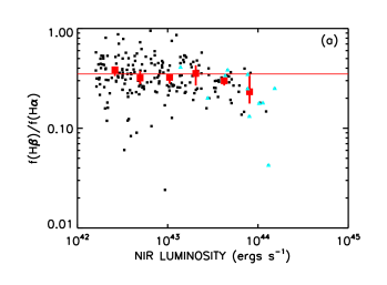
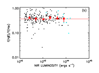
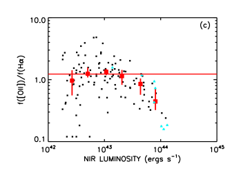
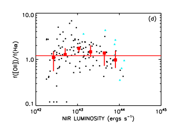
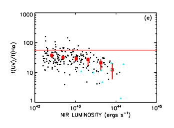
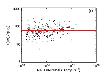
Figure 16.— In all panels we consider only galaxies in the low-$z$ sample with rest-frame EW(H$\alpha$$)>12$ Å. The large red squares denote the median values at each luminosity with $\pm 1\sigma$ errors computed using the median sign method. The 20 cm sources are denoted by cyan triangles. All ratios are plotted vs. NIR luminosity. (a) Balmer ratio. (b) Extinction corrected Balmer ratio. In these two panels the case B ratio in the absence of extinction is shown by the red horizontal line. (c) $f($[O$\thinspace{\rm II}]$$~{}\lambda 3727)/f($H$\alpha$). (d) Extinction corrected $f($[O$\thinspace{\rm II}]$$~{}\lambda 3727)/f($H$\alpha$). In these two panels the $f($[O$\thinspace{\rm II}]$$~{}\lambda 3727)/f($H$\alpha$) ratio used to compute the calibration of the [O$\thinspace{\rm II}]$$~{}\lambda 3727$ determined SFR is shown by the red horizontal line. (e) $f($UV$)/f($H$\alpha$) using the rest-frame UV flux defined in the text. (f) Extinction corrected $f($UV$)/f($H$\alpha$). In these two panels the $f($UV$)/f($H$\alpha$) ratio used to compute the calibration of the UV determined SFR is shown by the red horizontal line.

We next estimated the extinctions from the Balmer ratios for the low-$z$ sample with rest-frame EW(H$\alpha$$)>12$ Å and made a linear fit against the continuum extinctions. This gives the relation

$$E(B-V)_{\rm spectral}=0.0+(0.87\pm 0.18)E(B-V)_{\rm BC03}\,.$$ (2)

This suggests that the line extinction is, if anything, smaller than the continuum extinction, but that, within the errors, the two extinction measurements are consistent on average. We will therefore use the BC03 extinctions to deredden the line fluxes at higher redshifts. However, we will regularly check to make sure that this assumption is providing consistent results.

7. Star Formation Rates

7.1. Relative Calibrations

Extensive discussions of the calibrations of the star formation diagnostics can be found throughout the recent literature (e.g., Kennicutt 1998; Rosa-González et al. 2002; Hopkins et al. 2003; Kewley et al. 2004; Moustakas et al. 2006). However, for consistency, it is best to internally calibrate data sets where possible. We can do this using our low-$z$ sample.

In Figures 16c and 16e we show, respectively, $f$([O$\thinspace{\rm II}]$)$/f$(H$\alpha$) and $f$(UV)$/f$(H$\alpha$) versus NIR luminosity for the low-$z$ sample with rest-frame EW(H$\alpha$$)>12$ Å. Here we have defined the rest-frame UV luminosity as the integral over the frequency range $10^{15}$ to $1.5\times 10^{15}$ Hz (which corresponds to the wavelength range 1993 to 2990 Å) minus 0.03 of the NIR luminosity. The latter correction, the value of which was determined from absorption line galaxies in the sample, removes the contribution from the older stars in the galaxy. Since our shortest measured wavelength is the $U$-band centered at 3700 Å, determining the UV luminosity requires an extrapolation for the lowest redshift sources.

Similar to what we saw for the Balmer ratio, there is substantial extinction only in the highest NIR luminosity galaxies. In Figures 16d and 16f we plot the same ratios shown, respectively, in Figures 16c and 16e, but this time after applying our BC03 extinction corrections. Again the medians (red squares) are flattened out by the extinction corrections.

To obtain the SFR calibrations and to quantify the scatter in the flux ratios, in Figure 7.1 we show, respectively, the distribution of the extinction corrected logarithmic (a) Balmer ratios, (b) $f$([O$\thinspace{\rm II}]$)$/f$(H$\alpha$) ratios, and (c) $f$(UV)$/f$(H$\alpha$) ratios (black histograms), together with Gaussian fits to the distributions (purple dashed curves). The mean value of the extinction corrected Balmer ratios agrees precisely with the case B ratio (red line in Fig. 7.1a), illustrating how well the extinction corrections work. However, there is a symmetric scatter with a $1\sigma$ dispersion of 0.13 dex in the Balmer ratio about the case B value. We take this as a rough measure of the systematic and statistical errors in the extinction corrected flux determinations at the H$\beta$ wavelength relative to H$\alpha$.

Regarding the $f$([O$\thinspace{\rm II}]$)$/f$(H$\alpha$) ratio, it has been shown that there is a dependence of this ratio on the oxygen abundance (e.g., Kewley et al. 2004; Mouhcine et al. 2005; Moustakas et al. 2006). In fact, it can be seen from Figures 7.1b and 7.1c that the UV flux has a somewhat tighter relation to the H$\alpha$ flux than the [O$\thinspace{\rm II}]$ flux does, despite both the extrapolation made to shorter wavelengths for the lowest redshift sources to determine the UV flux and the larger wavelength separation of the UV from H$\alpha$ than of [O$\thinspace{\rm II}]$ from H$\alpha$ (which means any uncertainties in the extinction corrections would have a larger effect). In addition, there are no significant outliers in the $f$(UV)$/f$(H$\alpha$) ratios, unlike the case for the $f$([O$\thinspace{\rm II}]$)$/f$(H$\alpha$) ratios.

We can now use the flux ratios to determine the calibrations to star formation rates (SFRs). We use as our primary calibration the conversion of $L($UV) to SFR from the BC03 models. The calibration for any individual galaxy depends on the galaxy star formation history (SFH), but the ensemble average is well determined since it is simply the amount of UV light produced per unit mass of stars. Since our principal goal is to compute the universal SFH, this is the appropriate quantity to choose. For our definition of the rest-frame UV luminosity given above,

$$\log{\rm SFR}=-42.63+\log L({\rm UV})\,.$$ (3)

Here the SFR is in M${}_{\odot}$ per year and is computed for the Salpeter IMF used throughout this paper. $L$(UV) denotes the intrinsic (i.e., corrected for extinction) rest-frame UV luminosity and is in units of ergs s${}^{-1}$. Our UV calibration is slightly lower than the value of $-42.55$ that would be obtained from the commonly used relation given by Kennicutt (1998). The Kennicutt relation is appropriate for an individual galaxy undergoing constant star formation, which gives a lower UV flux per unit SFR.

Distribution of the logarithm of the extinction corrected ratio of (a) H$\beta$$~{}\lambda 4861$, (b) [O$\thinspace{\rm II}]$$~{}\lambda 3727$, and (c) rest-frame UV flux as defined in the text to the H$\alpha$$~{}\lambda 6563$ flux for the low-$z$ sample with rest-frame EW(H$\alpha$$)>12$ Å (black histograms). In each case the Gaussian fit is shown by the purple dashed curve. In (a) the red vertical line shows the case B value, which agrees precisely with the mean measured ratio.

We next compute the H$\alpha$ calibration relative to our UV calibration based on the data. We must be careful in our object selection here since there is a potential problem with using objects selected to have H$\alpha$ flux. This arises because the H$\alpha$ is produced by more massive and younger stars than those responsible for the UV light. As long as the SFR is smoothly changing with time, then this is not a large effect. However, if the galaxies undergo episodic bursts rather than a smooth evolution (as we shall argue is the case in §LABEL:seccolor), then we will bias this ratio since we will not count galaxies which still have substantial UV light but where H$\alpha$ producing stars are no longer present. The different time averaging present in the emission line and UV calibrations should be borne in mind when considering the SFR of individual galaxies, but it should average out in the ensemble.

We can properly calibrate the H$\alpha$/UV ratio by computing the average H$\alpha$/UV for a UV-selected sample, which will then include the all of the H$\alpha$ emitters as a subsample. Using the UV-selected sample we obtain

$$\log{\rm SFR}=-40.90+\log L({\rm H}\alpha)\,,$$ (4)

with a $1\sigma$ spread of 0.24 dex. This differs by 0.2 dex from the value of $-41.1$ given in Kennicutt (1998) and is also higher than the value that would be derived from the BC03 models. (The H alpha luminosity for the BC03 models is derived from the ionizing photon production assuming this is fully absorbed in the galaxy.) This is not a consequence of the extinction model, since even using the unreddened values only reduces our value to $-41.03$.

This result can be restated as the sample having too much UV light relative to H$\alpha$ for the adopted IMF. The H$\alpha$ production is dominated by the most massive stars, and it is probable that the high UV/H$\alpha$ ratio is a consequence of differences in the true high-end IMF relative to that used in the models. As we noted in the introduction all of the currently used IMFs have similar high mass slopes and so would not change this result. Rather we need more intermediate mass stars relative to the very high mass end in the IMF. Fardal et al. (2007) describe this type of IMF as ”paunchy” and as we shall discuss later it can resolve a number of additional problems in making a consistent interperetation of the data set.

From the mean value of the logarithmic $f$(H$\beta$)$/f$(H$\alpha$) ratio, which is just the case B value (see Fig. 7.1), we find the calibration of Equation 4 can be translated to

$$\log{\rm SFR}=-40.45+\log L({\rm H}\beta)\,,$$ (5)

with a $1\sigma$ spread of 0.13 dex. H$\beta$ is often avoided as a SFR diagnostic because of concerns about the contamination by the underlying stellar absorption. However, with such a low $1\sigma$ spread for our low-$z$ sample, it appears to be quite a good diagnostic.

From Figure 7.1 we saw that the UV flux provided a better estimate of the SFR than the [O$\thinspace{\rm II}]$ flux did. The average calibration for [O$\thinspace{\rm II}]$, using the mean value of the logarithmic $f$([O$\thinspace{\rm II}]$)$/f$(H$\alpha$) ratio, is

$$\log{\rm SFR}=-41.03+\log L({\rm[OII]}~{}\lambda 3727)\,,$$ (6)

with a $1\sigma$ spread of 0.26 dex. This may be compared with the value of $-40.85$ given in Kennicutt (1998).

Ratio of the [O$\thinspace{\rm II}]$ SFR to the H$\alpha$ SFR versus the H$\alpha$ SFR (all extinction corrected) for the low-$z$ sample with EW(H$\alpha$$)>12$ Å and $\log({\rm SFR}({\rm H}\alpha))>-0.5$ (black squares). The black dotted line shows the least-square polynomial fit with a gradient of $-0.09$ dex per dex.

The broader spread in the [O$\thinspace{\rm II}]$ calibration is reflected in its systematic dependence on the galaxy properties. In Figure 7.1 we show the weak dependence of the ratio of the [O$\thinspace{\rm II}]$ SFR to the H$\alpha$ SFR on the H$\alpha$ SFR (all extinction corrected). There is a $0.09\pm 0.05$ dex decline per dex increase in the H$\alpha$ SFR, which is slightly larger than the locally measured $0.03\pm 0.02$ dex decline per dex increase in the H$\alpha$ SFR measured to somewhat lower H$\alpha$ SFRs (Kewley et al. 2004) but consistent within the errors. We show in §7.2 that the dependence of the SFR ratio on the mass of the galaxy is even stronger than its dependence on the H$\alpha$ SFR of the galaxy.

Given the larger scatter and systematic dependences of the [O$\thinspace{\rm II}]$ calibration, we will adopt the UV calibration as our primary calibration.

7.2. Comparisons Using the Mid-$z$ Sample

We next tested the relative [O$\thinspace{\rm II}]$ and H$\beta$ calibrations against our primary UV calibration over the wider redshift range of the full mid-$z$ sample ($z<0.9$). In Figure 7.2a we plot the ratio of the [O$\thinspace{\rm II}]$ SFR to the UV SFR (both extinction corrected) versus galaxy mass. We show the lower redshift sources ($z=0.05-0.475$) with red diamonds and the higher redshift sources ($z=0.475-0.9$) with black squares, and we only show the results above the mass at which each redshift range is complete. The ratio changes slowly with both mass and redshift. The change is a 0.19 dex decline per dex increase in mass and a 0.04 dex increase between the low and high redshift ranges. This probably primarily reflects the higher metallicity in the more massive galaxies and the increase of metallicity to lower redshifts, which results in temperature changes in the H II regions and the [O$\thinspace{\rm II}]$ line being stronger relative to the primary H$\alpha$ line. Thus, if we were to use our [O$\thinspace{\rm II}]$ calibration, we would find it difficult to study the evolution of the SFRs as a function of redshift, mass, and metallicity.

In contrast, as shown in Figure 7.2b (same symbols as in Fig. 7.2a), the ratio of the H$\beta$ SFR to the UV SFR (both extinction corrected) varies more slowly with galaxy mass and does not vary significantly with redshift. The change with mass is a 0.11 dex decline per dex increase in galaxy mass. Thus, H$\beta$ can also be used over the $z=0.05-0.9$ range where it can be measured.

(a) Ratio of the [O$\thinspace{\rm II}]$ SFR to the UV SFR (both extinction corrected) vs. galaxy mass. (b) Ratio of the H$\beta$ SFR to the UV SFR (both extinction corrected) vs. galaxy mass. Only sources with EW(H$\beta$$)>4$ Å are included. The red diamonds (black squares) show the results for $z=0.05-0.475$ ($z=0.475-0.9$). We show the results only above the mass at which each redshift interval is complete. The least-square polynomial fits are shown with the dashed red (solid black) lines for the $z=0.05-0.475$ ($z=0.475-0.9$) sample. The one AGN based on its X-ray luminosities is enclosed in the large red diamond and is excluded from the fits. In (a) there is a significant gradient with mass and a small amount of evolution between the two redshift samples. In (b) there is a smaller change with galaxy mass and no significant evolution between the two redshift samples.

7.3. Comparison with 24 $\mu$m

Using the observed-frame 24 $\mu$m fluxes of the galaxies is a relatively poor way to determine the FIR luminosities and hence SFRs of the galaxies (e.g., Dale et al. 2005). However, because of the ready availability of 24 $\mu$m data from the Spitzer MIPS observations, this has become a common way of estimating SFRs, and nearly all of the papers that we will compare with use some version of this method to determine their SFRs. We therefore compare with 24 $\mu$m determined SFRs here.

We compute the $24~{}\mu$m SFRs following the presciption given in Conselice07. We use the Dale & Helou (2002) SEDs to convert the 24 $\mu$m flux to FIR luminosity following Figure 7 of Le Floc’h et al. (2005). We then use the Bell et al. (2005) relation between the reradiated SFR and the FIR luminosity (converted to the Salpeter IMF of the present paper),

$$\log{\rm SFR}=-43.36+\log L(FIR)\,,$$ (7)

to compute the SFRs.

In Figure 7.3 we compare the SFRs determined from the $24~{}\mu$m fluxes with the reradiated SFRs determined from the UV luminosities. (Here the reradiated SFR is the difference between the SFR computed after correcting for extinction and the SFR computed without an extinction correction.) In each redshift interval we only show the sources with sufficiently high SFRs that they will lie above the 80 $\mu$Jy sensitivity of the $24~{}\mu$m observations.

Ratio of the 24 $\mu$m SFR to the reradiated UV SFR vs. the reradiated UV SFR. The sources are separated by redshift interval and are only shown if their SFR is above the SFR where the galaxies will be detected at the flux limit for the $24~{}\mu$m sample. Squares correspond to $z=0.05-0.475$ and are shown above 10 M${}_{\odot}$ yr${}^{-1}$, diamonds correspond to $z=0.475-0.9$ and are shown above 30 M${}_{\odot}$ yr${}^{-1}$, and triangles correspond to $z=0.9-1.5$ and are shown above 100 M${}_{\odot}$ yr${}^{-1}$. Sources containing an AGN based on their X-ray luminosities are enclosed in larger red diamonds.

While there is a considerable spread in the individual SFR ratios, there is no clear dependence on redshift or on SFR. The normalization difference between the two methods is only $-0.08$ dex in the ensemble average, which is well within the uncertainties in the calibrations. The ensemble distribution is symmetric about the average with a $1\sigma$ multiplicative spread of 0.29 dex. Thus, while there is a substantial spread in the individual galaxy determinations, the two methods give good agreement when applied to the galaxy population as a whole. Excluding AGNs based on their X-ray properties (i.e., sources enclosed in red diamonds in Figure 7.3) has no effect on the relative calibration.

8. Metallicities in the Emission Line Galaxies: The Low-$z$ Sample

We may construct a number of emission line diagnostics for the low-$z$ sample, since many of the spectra cover all of the emission lines from [O$\thinspace{\rm II}]$ to [S$\thinspace{\rm II}]$. We therefore begin with a comparison of the metallicity-luminosity and metallicity-mass relations for these sources before proceeding to the mid-$z$ sample in §9. We know that the [S$\thinspace{\rm II}]$ratios place most of the galaxies in the low-density regime, but we do not use this information further.

8.1. [NII]/[OII] Diagnostic Ratio

Kewley & Dopita (2002; hereafter KD02) advocate the use of the N2O2 $=f($[N$\thinspace{\rm II}]$$)/f($[O$\thinspace{\rm II}]$) diagnostic ratio whenever possible, since this ratio is quite insensitive to the ionization parameter $q$ and has a strong dependence on metallicity above $\log$(O/H)$+12\sim 8.5$. However, the downside of this diagnostic ratio is that it compares two widely separated lines where the uncertainties in the flux calibration and extinction are more severe. Throughout this section we use the BC03 extinctions of §4.

Logarithmic (a) extinction uncorrected and (b) extinction corrected N2O2 diagnostic ratio vs. NIR luminosity for the sources in the low-$z$ sample with EW(H$\alpha$$)>12$ Å and an [O$\thinspace{\rm II}]$ line that can be measured (black squares). The sources with a flux ratio less than 0.015 are plotted at that value ($-1.82$ in the logarithm). In each panel the solid line shows the least-square polynomial fit to all the data, and the dashed line shows the least-square polynomial fit to only the data with NIR luminosities in the range $10^{43}-10^{44}$ ergs s${}^{-1}$.

In Figure 8.1 we plot (a) extinction uncorrected and (b) extinction corrected N2O2 versus NIR luminosity for the 115 sources in the low-$z$ sample with EW(H$\alpha$$)>12$ Å and an [O$\thinspace{\rm II}]$ line that can be measured (it can be negative). These sources cover the redshift range $z=0.2-0.475$ and have a median redshift of $z=0.4$. We find a strong correlation between N2O2 and NIR luminosity. For each panel in Figure 8.1 we use a solid line to show the least-square polynomial fit to all the data. In the faintest sources the $f($[N$\thinspace{\rm II}]$) and $f($[O$\thinspace{\rm II}]$) are weak, which results in larger scatter. For example, the extreme up-scattered point at low NIR luminosity in Figure 8.1 is a source with very weak $f($[N$\thinspace{\rm II}]$) and $f($[O$\thinspace{\rm II}]$). Thus, for each panel we also do a fit to the data in the restricted NIR luminosity range $10^{43}-10^{44}$ ergs s${}^{-1}$ to minimize these effects (dashed line). The relation for the extinction corrected data restricted in luminosity is

$$\log({\rm N2O2})=-0.94+(0.63\pm 0.08)\log(L_{N})\,,$$ (8)

where $L_{N}$ is the NIR luminosity in units of $10^{43}$ ergs s${}^{-1}$.

Metallicity determined from the (a) extinction uncorrected and (b) extinction corrected N2O2 diagnostic ratio vs. galaxy mass for the sources in the low-$z$ sample with EW(H$\alpha$$)>12$ Å and an [O$\thinspace{\rm II}]$ line that can be measured (black squares). The conversion is for an ionization parameter $q=4\times 10^{7}$ cm s${}^{-1}$, but the conversion is insensitive to this choice. In each panel the black solid line shows the least-square polynomial fit to all the data, and the red dotted ine shows the solar abundance.

We use the KD02 calibration (their Eq. 4 and Table 3) to convert our N2O2 values to metallicities, assuming an ionization parameter $q=2\times 10^{7}$ cm s${}^{-1}$. This $q$ value is typical of the ionization parameters in our galaxies (see §8.2). However, the present conversion is extremely insensitive to the choice of $q$. In Figure 8.1 we plot metallicity determined from (a) extinction uncorrected and (b) extinction corrected N2O2 versus galaxy mass. For each panel we use a solid line to show the least-square polynomial fit to all the data. The metallicity-mass relation for the extinction corrected case is

$$12+\log({\rm O/H})=8.75+(0.44\pm 0.06)\log(M_{10})\,,$$ (9)

where $M_{10}$ is the galaxy mass in units of $10^{10}$ M${}_{\odot}$. The extinction corrections flatten the slope (the unextinguished slope is $0.52\pm 0.06$) since they reduce the N2O2 values more substantially in the high mass (high NIR luminosity) galaxies than they do in the lower mass galaxies.

8.2. Ionization Parameter

We can now combine the metallicities determined from extinction corrected N2O2 with extinction corrected O32 $=1.3\times f$([O$\thinspace{\rm III}]$)$/f$([O$\thinspace{\rm II}]$) to determine the ionization parameters $q$. Here we do so using the KD02 parameterization of the O32 dependence on $q$ and metallicity. We plot $q$ versus NIR luminosity in Figure 8.2. The $q$ values lie in a surprisingly small range around a median value of $2.2\times 10^{7}$ cm s${}^{-1}$, with more than 77% lying within a multiplicative factor of 2 of this value. There also appears to be little dependence of $q$ on NIR luminosity.

Ionization parameter obtained by combining the metallicity determined from the extinction corrected N2O2 diagnostic ratio with the extinction corrected O32 diagnostic ratio vs. NIR luminosity (black squares). The effects of the extinction correction are to slightly reduce the average ionization parameter and also to flatten the dependence on luminosity. Most of the sources lie in the $q=1-4\times 10^{7}$ cm s${}^{-1}$ range with an average value of $q=2.2\times 10^{7}$ cm s${}^{-1}$. The black solid line shows the least-square polynomial fit. The ionization parameter shows little dependence on NIR luminosity.

8.3. [NII]/[H$\alpha$] Diagostic Ratio

The tightly determined $q$ values mean that other diagnostic ratios, such as NH = $f$([N$\thinspace{\rm II}]$)$/f$(H$\alpha$), which normally have too much dependence on ionization parameter to be useful, actually work surprisingly well. Because [N$\thinspace{\rm II}]$ and H$\alpha$ are extremely close in wavelength, NH is not dependent on the extinction corrections nor on the flux calibration methodology and thus provides a powerful check on the metallicities computed from N2O2. In Figure 8.3 we show NH versus NIR luminosity. There is a strong correlation, which we fit over the NIR luminosity range $10^{43}-10^{44}$ ergs s${}^{-1}$ with the solid line.

We next constructed the metallicity-mass relation from NH using Eq. 12 of Kobulnicky & Kewley (2004; hereafter, KK04) and $q=2\times 10^{7}$ cm s${}^{-1}$. (We note that the use of the coefficients given in Table 3 of KD02 for NH appears to give results that are inconsistent with Figure 7 of KD02 and Eq. 12 of KK04.) The metallicity-mass relation,

$$12+\log({\rm O/H})=8.85+(0.36\pm 0.04)\log(M_{10})\,,$$ (10)

is shown in Figure 8.3 by the black solid line. Recomputing the data points using higher ($q=4\times 10^{7}$ cm s${}^{-1}$) or lower ($q=10^{7}$ cm s${}^{-1}$) ionization parameters and fitting the revised data points (red dash-dotted lines) does not substantially change the slope, but it does significantly change the normalization.

Logarithmic NH diagnostic ratio vs. NIR luminosity for the sources in the low-$z$ sample with EW(H$\alpha$$)>12$ Å (black squares). The black solid line shows the least-square polynomial fit to the data.

Metallicity based on the NH diagnostic ratio vs. galaxy mass for the sources in the low-$z$ sample with EW(H$\alpha$$)>12$ Å computed for an ionization parameter of $q=2\times 10^{7}$ cm s${}^{-1}$ (black squares). The black solid line shows the least-square polynomial fit to the data. The red dash-dotted lines show the fits which would be obtained for $q=4\times 10^{7}$ cm s${}^{-1}$ (upper line) and $q=10^{7}$ cm s${}^{-1}$ (lower line). The cyan dashed line shows the metallicity-mass relation derived from the extinction corrected N2O2 diagnostic ratio (Eq. 9). The red dotted horizontal line shows the solar metallicity.

In the figure we compare the metallicity-mass relation of Eq. 10 (black solid line) with the metallicity-mass relation of Eq. 9 (cyan dashed line) derived from N2O2. The agreement is reasonable given the sensitivity of the NH diagnostic to the ionization parameter. The mean metallicity in the $10^{10}$ to $10^{11}$ M${}_{\odot}$ range is 9.03 from NH and 8.99 from N2O2, which reassuringly shows that the metallicity and ionization parameter determinations are roughly self-consistent and that our treatment of the extinctions is plausible.

8.4. R23 Diagnostic Ratio

(a) Logarithmic R23 vs. metallicity for the McGaugh (1991) models corresponding to $\log({\rm O32})=-1$ (red dashed), $-0.25$ (black solid), and 0.5 (blue dotted). These values cover the range of our data. (b) Logarithmic extinction corrected R23 vs. logarithmic extinction corrected O32 for the sources in the low-$z$ sample with EW(H$\beta$$)>4$ Å and detected [O$\thinspace{\rm II}]$ (black squares). Tracks give the R23-O32 relations from McGaugh (1991): purple dashed lines show the relation on the low metallicity branch for three values of $12+\log({\rm O/H})$ [8.0 (lowest curve), 8.2, and 8.4 (highest curve)], and solid black lines show the relation on the high metallicity branch for five values of $12+\log({\rm O/H})$ [8.4 (highest curve), 8.6, 8.8, 9.0, and 9.1 (lowest curve)]. On the high metallicity branch there is little dependence of R23 on O32.

The R23 diagnostic ratio [$1.3\times f($[O$\thinspace{\rm III}]$$~{}\lambda 5007)+f($[O$\thinspace{\rm II}]$$~{}\lambda 3727)]/f($H$\beta$) of Pagel et al. (1979) is one of the most frequently used metallicity diagnostics. It can be measured in our data out to $z=0.9$. However, it is unfortunately multivalued with both a low metallicity and a high metallicity branch. Thus, the same value of R23 can correspond to two substantially different metallicities. Moreover, R23 is only weakly dependent on metallicity for $12+\log({\rm O/H})\lesssim 8.6$. We can see these traits in Figure 8.4. In Figure 8.4a we plot logarithmic R23 versus metallicity for the McGaugh (1991) models corresponding to $\log({\rm O32})=-1$ (red dashed), $-0.25$ (black solid), and 0.5 (blue dotted). These cover the range of ionization dependent O32 measurements from our data, as can be seen from Figure 8.4b where we plot logarithmic extinction corrected R23 versus logarithmic extinction corrected O32 for the 164 sources in the low-$z$ sample with EW(H$\beta$$)>4$ Å and detected [O$\thinspace{\rm II}]$ (black squares). Here we overlay the models of McGaugh (1991) for the low metallicity branch (purple dashed) and the high metallicity branch (black solid) onto the data.

Unfortunately, much of the data in Figure 8.4b lie near the peak of the R23 ratio [$\log$(R23) in the range 0.5 to 1], where R23 is a relatively slowly varying function of the metallicity and where the metallicity could lie on either the upper or lower branches (see Fig. 8.4a). Fortunately, however, we can see from Figures 8.1 and 8.3 (where the metallicities were computed from N2O2 and NH, respectively) that the galaxies in the low-$z$ sample with masses greater than $2\times 10^{9}$ M${}_{\odot}$ primarily lie on the high metallicity branch of the R23 diagnostic ratio [$12+\log({\rm O/H})>8.4$] (see also KK04). In §9 we will assume that the higher redshift $(z>0.475)$ sources contained in the mid-$z$ sample also predominantly lie on the high metallicity branch, though if there is significant metallicity evolution, this assumption could break down.

With most of the galaxies on the upper branch, the interpretation is considerably simplified, since on this branch there is very little dependence on O32. From the McGaugh (1991) models in Figure 8.4, we can see that at metallicities of $12+\log({\rm O/H})>8.6$, the R23 parameter is nearly ionization independent and has a steep dependence on metallicity. We can therefore make a simple investigation of the metal evolution by analyzing the dependence of R23 on the NIR luminosity without considering O32. In Figure 8.4 we show the dependence of extinction corrected R23 on NIR luminosity for the low-$z$ sample with EW(H$\beta$$)>4$ Å and detected [O$\thinspace{\rm II}]$. The median R23 is relatively flat at lower luminosities and then drops at the higher luminosity end. The least-square polynomial fit is

$$\log({\rm R23})=0.61-(0.08\pm 0.04)\log(L_{N})\,.$$ (11)

The extinction corrected R23 diagnostic ratio vs. NIR luminosity for the low-$z$ sample with EW(H$\beta$$)>4$ Å and detected [O$\thinspace{\rm II}]$ (black squares). The black solid line shows the least-square polynomial fit.

We can now also translate R23 and O32 to metallicity using the KK04 calibration (their Eq. 18), which is an average of the McGaugh (1991) and the KD02 R23 methods and is only valid for the upper branch. The dependence of the metallicity on the mass is then given by

$$12+\log({\rm O/H})=8.77+(0.23\pm 0.05)\log(M_{10})\,,$$ (12)

which we show with a black solid line in Figure 8.4. Alternatively, we can translate R23 alone to $12+\log({\rm O/H})$ using Equation 1 of Tremonti et al. (2004; hereafter, Tremonti04), which is an analytical fit to their R23-metallicity relation and is also only valid for the upper branch. In this case we find for the dependence of the metallicity on the mass

$$12+\log({\rm O/H})=8.78+(0.24\pm 0.05)\log(M_{10})\,,$$ (13)

which has a very similar slope to Equation 12 and, over the mass range $10^{10}$ to $10^{11}$ M${}_{\odot}$, only differs in the intercept by 0.01 dex.

$12+\log({\rm O/H})$ computed from the extinction corrected R23 and O32 diagnostic ratios using the KK04 calibration vs. galaxy mass for the low-$z$ sample with EW(H$\beta$$)>4$ Å and detected [O$\thinspace{\rm II}]$ (black squares). The black solid line shows the least-square polynomial fit (Eq. 12), which is flatter than the fits to the metallicities derived from the extinction corrected N2O2 diagnostic ratio (Eq. 9; cyan dotted line) and the NH diagnostic ratio (Eq. 10; red dashed line). The red dotted line shows the solar abundance.

In Figure 8.4 we compare the fit to the metallicities derived from R23 and O32 using the KK04 calibration (black solid line) with the fits to the metallicities derived from N202 (cyan dotted line) and NH (red dashed line). While the metallicities are close, using R23 gives a shallower slope, as can be seen quantitatively by comparing Equation 12 with Equations 9 and 10. The shallower slope is most likely a consequence of our assumption that the bulk of the sources lie on the high metallicity branch of R23. This assumption breaks down at the low mass end, causing some of the low metallicity branch points to be assigned artificially high metallicities.

We also calculated the values of the ionization parameter $q$ from R23 and O32 using the new parameterizations of KK04 (their Eqs. 13 and 17) for the KD02 models. (Note that KK04 did not give a parameterization for $q$ for their averaged KD02 and M91 R23 method, which we used to compute the metallicities in Figure 8.4. However, since $q$ is not particularly sensitive to metallicity, the fact that we are using the updated KD02 parameterizations here to calculate the $q$ values should not be important.) These $q$ values are very similar to those derived from N2O2. The median $q=2.3\times 10^{7}$ cm s${}^{-1}$, and 80% of the sample lies between $q=1.1\times 10^{7}$ cm s${}^{-1}$ and $q=4.4\times 10^{7}$ cm s${}^{-1}$.

9. Metallicities in the Emission Line Galaxies: The [OIII] Sample

At higher redshifts only the R23 diagnostic ratio can be computed from the optical spectra. As can be seen from Figure 8.4 (and as we discussed in §8.4), this results in some ambiguities in calculating the metallicities since R23 is relatively insensitive to metallicity at sub-solar values, and the translation from R23 to metallicity requires assumptions about which branch of the R23 relation the metallicity is on. We therefore first analyze the raw R23 evolution without making any translation to metallicity.

In Figure 9 we show the dependence of R23 on redshift for the mid-$z$ sample with EW(H$\beta$$)>4$ Å and detected [O$\thinspace{\rm II}]$. We have divided the sample into three NIR luminosity intervals: (a) $(5-20)\times 10^{43}$ ergs s${}^{-1}$; (b) $(2-5)\times 10^{43}$ ergs s${}^{-1}$; and (c) $(0.8-2)\times 10^{43}$ ergs s${}^{-1}$. The purple solid line shows the least-square polynomial fit to the data in (c). This same fit is also shown as a purple line in (a) and (b) for comparison with the fit to the data in each of those intervals (black solid line). In all three luminosity intervals we see a similar evolution with redshift, with R23 increasing by about $0.2-0.3$ dex between $z=0.3$ and $z=0.9$. The parallel evolution of the three luminosity intervals indicates that the shape of the metallicity-mass relation does not evolve rapidly with redshift over this redshift range. This result is not changed if we exclude the strong redshift filament seen at $z=0.85$. Since R23 decreases with increasing metallicity on the high metallicity branch (see Fig. 8.4a), we also see from Figure 9 that high luminosity galaxies have higher metallicities than lower luminosity galaxies at all redshifts. Moreover, in a given luminosity interval, the metallicity is increasing with decreasing redshift. The dependence of the metallicity on redshift is sufficiently strong that high luminosity galaxies at high redshifts have comparable metallicities to low luminosity galaxies at lower redshifts.

We may now compute the metallicity evolution with redshift and luminosity more directly at the expense of both assuming that the metallicity is on the upper branch of the R23 relation and adopting a specific calibration to metallicity. In Figure LABEL:metal we show $12+\log({\rm O/H})$ computed from R23 and O32 in the same manner as in §8.4 using the KK04 calibration. The points are separated into the redshift intervals $z=0.05-0.475$ (red diamonds) and $z=0.475-0.9$ (black squares) with median redshifts of 0.44 and 0.75. Even over this relatively narrow redshift range the average metallicity has dropped by about 0.13 dex. Both distributions show an upper envelope of $12+\log({\rm O/H})\sim 9.1$. The spread to lower metallicities at the higher redshifts should not be taken seriously as it is a consequence of applying the high metallicity branch equation to galaxies that are on the low metallicity branch. We find the least-square polynomial fit to the metallicities, NIR luminosities, and $(1+z)$ values for all the galaxies together to be

$$12+\log({\rm O/H})=8.95+0.18\log(L_{N})-1.52\log(1+z)\,,$$ (14)

which we show in Figure LABEL:metal calculated at the median redshifts of $0.44$ (red solid) and $0.75$ (black solid), respectively. We also show the least-square polynomial fits to the metallicities and NIR luminosities for $z=0.05-0.475$ (red dashed) and $z=0.475-0.9$ (black dashed).

Logarithmic extinction corrected R23 vs. redshift for the mid-$z$ sample with EW(H$\beta$$)>4$ Å and detected [O$\thinspace{\rm II}]$ for three NIR luminosity ranges: (a) $(5-20)\times 10^{43}$ ergs s${}^{-1}$, (b) $(2-5)\times 10^{43}$ ergs s${}^{-1}$, and (c) $(0.8-2)\times 10^{43}$ ergs s${}^{-1}$. Each panel is marked with the luminosity range in units of $10^{43}$ ergs s${}^{-1}$. In (a) and (b) the black solid line shows the least-square polynomial fit to $\log($R23) vs. $\log(1+z)$. In (a), (b), and (c) the purple solid line shows the least-square polynomial fit to the data in (c).