Many-Body Approximations in the sd-Shell Sandbox

Abstract

A new theoretical approach is presented that combines the Hartree-Fock variational scheme with the exact solution of the pairing problem in the finite orbital space. Using this formulation in the $sd$-space as an example, we show that the exact pairing significantly improves the results for the ground state energy.

I Introduction

The classical Hartree-Fock (HF) approximation is a prototype of the modern approach to the quantum many-body problem related to the energy density functional KS65 ; dreizler90 . When applied to complex nuclei, the density functional theory may provide a universal description across the nuclear chart. The pairing interaction that is present in nuclei as well as in fermionic condensed matter systems is usually included in the Hartree-Fock-Bogoliubov (HFB) form goodman79 . The well known deficiencies of the HFB approach for mesoscopic systems follow mainly from its non-conservation of particle number. As a result, unphysical features are introduced into dynamics, the superfluid phase transition appears too sharp, and the correlational energy produced by pairing might be severely underestimated. As was shown earlier VBZ01 ; ZV03pairing , the pairing part of the problem can be solved numerically quite easily with the help of the seniority representation in a spherical basis, and its exact solution significantly improves the results.

It was also sketched in VBZ01 how other parts of the interaction can be incorporated into the exact pairing method in the approximate way that reminds the HF approach. This can be done in an iterative fashion: the exact pairing solution using the starting single-particle basis determines the actual occupation numbers; these (in general, fractional) occupancies self-consistently determine, in the HF spirit, an improved single-particle basis where we again solve the pairing problem etc. until convergence. In this way both mean-field features, deformation and pairing, are accounted for. The main purpose of the current work is to further develop this Hartree-Fock plus pairing correlation (HFP) method that essentially is an intermediate step from the HF approach towards the full shell-model (SM) description. On one hand, we would want to keep the simplicity and modest computer demands as inherent properties of the mean field approach. On the other hand, we take into consideration pairing and other physical effects beyond the simple HF, or mean field in general. We check our approach for the $sd$-shell nuclei, where the SM with large-scale diagonalization works perfectly sdsm and can serve as a searchlight illuminating the correct direction of motion. The success of this attempt will allow the extension of the approach to heavy nuclei, where the catastrophic growth of dimensions makes the complete shell model solution unrealistic.

II Outline of the method

As in most mean-field approaches, we formulate this method as variational one. As in the shell model, we assume a general form of the two-body Hamiltonian that includes the single-particle term $t$ and the (antisymmetrized) two-body interaction $V$:

$$\hat{H}=\sum_{ik}t_{ik}\,a^{\dagger}_{i}a_{k}+\frac{1}{4}\,\sum_{ijkl}V_{ijkl}\,a_{i}^{\dagger}a_{j}^{\dagger}a_{k}a_{l}.$$ (1)

The variational wave function $|\Psi\rangle$ will be defined below. The wave function and all properties of the system follow from the minimization of the expectation value

$$\langle\Psi|\hat{H}|\Psi\rangle.$$ (2)

For our test of the methods, we will take for $V$ the USDB interaction from the $sd$-shell model sdsm . It will allow us to compare the results obtained using our approximate method with the exact shell model calculations in the same single-particle model space.

The ground state wave function $|\Psi\rangle$ for a fixed particle number $N$ can be presented as a superposition of basis states,

$$|\Psi\rangle=\sum_{d\in{\sl D}}C_{d}|d\rangle,$$ (3)

where each basis state $|d\rangle$ is a Slater determinant which for $N$ fermions can be written as usual:

$$|d\rangle=a^{\dagger}_{\nu_{1}}a^{\dagger}_{\nu_{2}}\dots a^{\dagger}_{\nu_{N}}|0\rangle.$$ (4)

The single-particle states $\phi_{\nu}$ can be found with the help of the variational principle as it is usually done in the HF method. The approach is actually defined by the selection of the space $D$ spanned by the determinants $|d\rangle$. If we choose only one Slater determinant as our variational wave function (3), we come to the standard HF approximation. If the manifold $D$ includes all possible configurations, then we get the exact shell-model solution.

In this article our choice is determined by the pairing phenomenon which smears the Fermi surface and converts the Fermi-gas ground state into a superposition of Slater determinants. In the case of a spherical system with the pairing forces taken as the $J=0,T=1$ part of the two-body interaction (1), we have seniority $s$ as a good quantum number. For an even number of particles, the ground state has $s=0$, while for an odd number $s=1$. In this simple case we can construct the basis of Slater determinants $|d\rangle$ occupying single-particle levels $|jm\rangle$ by pairs,

$$\prod_{j;m>0}a_{jm}^{\dagger}a_{j\tilde{m}}^{\dagger}|0\rangle,$$ (5)

where $a_{j\tilde{m}}^{\dagger}=(-1)^{j-m}a_{j-m}^{\dagger}$ is the creation operator for the time-conjugate single-particle state with respect to $a_{jm}^{\dagger}$. Here we omit all quantum numbers except total angular momentum $j$ and its projection $m$.

The presence of other types of the interaction in general breaks spherical symmetry and brings in the deformed mean field. In the case of a deformed nucleus, even if we had had only $J=0$ part of the two-body interaction (1) in the spherical representation, we have to take into consideration a broader class of pairs arising as a result of splitting and mixing of the original spherical states by deformation. Here we limit ourselves by the case of axially symmetric deformation, when the single-particle orbitals $|\nu m\rangle$ are still characterized by the angular momentum projection $m$ along with other quantum numbers $\nu$.

According to the Kramers theorem, the orbitals $|\nu m\rangle$ and $|\nu-m\rangle$ are degenerate. However, the pairs may also be formed by the states $m$ and $-m$ belonging to different sets of remaining quantum numbers. Thus, for our basis Slater determinants $|d\rangle$ we assume the following form:

$$\prod_{\nu,\kappa;m>0}a_{\nu m}^{\dagger}a_{\kappa-m}^{\dagger}|0\rangle.$$ (6)

We construct the variational wave function (3) as a superposition of the Slater determinants (6) for a given particle number. Using such a form we hope to correctly account for pairing correlations in the deformed case at the same time crucially reducing the dimension of space $D$ in comparison with the full shell model. Actually prescriptions (5,6) are valid only for an even number of particles. For an odd particle number, we use the same eq. (6) but add one additional creation operator that corresponds to the odd particle. The odd particle can be placed in any empty single-particle state, and the states are divided into classes with a definite value of the angular momentum projection.

In the current application of our method we make a simplifying approximation treating protons and neutrons separately. It means that, though we consider the full two-body interaction (1) including $T_{z}=0$ part, the variational function (3) is constructed as the product of proton and neutron parts. Clearly we are losing here proton-neutron correlations although their mutual contributions to the mean field are fully accounted for.

The variation over amplitudes $C_{d}$ with the additional normalization condition of the wave function, $\langle\Psi|\Psi\rangle=1$, leads us to the usual set of equations,

$$\sum_{d^{\prime}}\langle d|\hat{H}|d^{\prime}\rangle C_{d^{\prime}}=EC_{d}.$$ (7)

The matrix elements $\langle d|\hat{H}|d^{\prime}\rangle$ are calculated for the determinants built on a given single-particle basis, and equations (7) are solved numerically. The mean-field basis is found from the self-consistent HF equations:

$$h(\rho)\phi_{\nu}=\epsilon_{\nu}\phi_{\nu},$$ (8)

where

$$h(\rho)=t+V(\rho)$$ (9)

is the single-particle HF Hamiltonian, $\epsilon_{\nu}$ are the single-particle energies, and $\rho$ is the density matrix self-consistently determined by

$$\rho_{ij}=\langle\Psi|a^{\dagger}_{j}a_{i}|\Psi\rangle.$$ (10)

The mean field potential is given by its matrix elements,

$$V_{ij}(\rho)=\sum_{kl}V_{iklj}\rho_{lk}.$$ (11)

In this conventional mean field formulation, the potential (11) contains the direct and exchange contributions. The pairing effects, with strict particle number conservation, are contained in the superposition of the Slater determinants (2) used instead of the single HF determinant. The whole construction can be further improved by using the exact but more complicated variational approach relating the single-particle basis to the full set of the coefficients of the superposition (2). Such a possibility will be considered in the future.

The HFP scheme of solution is the following:

• Start with the spherical single-particle basis $|\kappa m\rangle$

• Choose in this basis the initial diagonal density matrix $\rho$ corresponding to occupation numbers specific for prolate or oblate shapes (pairs with small or large $|m|$, respectively)

• Solve the HF variational equation (8) and get the single-particle spectrum ($\phi_{\nu},\epsilon_{\nu}$), in general corresponding to a deformed field

• Construct the “paired” class of many-body basis wave functions according to eq. (6) and calculate the matrix elements of the Hamiltonian $H$

• Solve the variational equation (7) and obtain the ground state wave function

• Calculate the next-step density matrix (10)

• Repeat the procedure starting from the step three until convergence

The converged results will certainly be a local minimum of eq. (2). Exploration of different starting choices in step 2 is needed to find a global minimum. In our study here we start with a spherical single-particle basis (because the USDB interaction is so defined) but in principle any convenient axial basis could be used. In the end, the ground state energy can be found as the Hamiltonian expectation value over the resulting ground state wave function $|\Psi\rangle$,

$$E_{{\rm HFP}}=\langle\Psi|\hat{H}|\Psi\rangle.$$ (12)

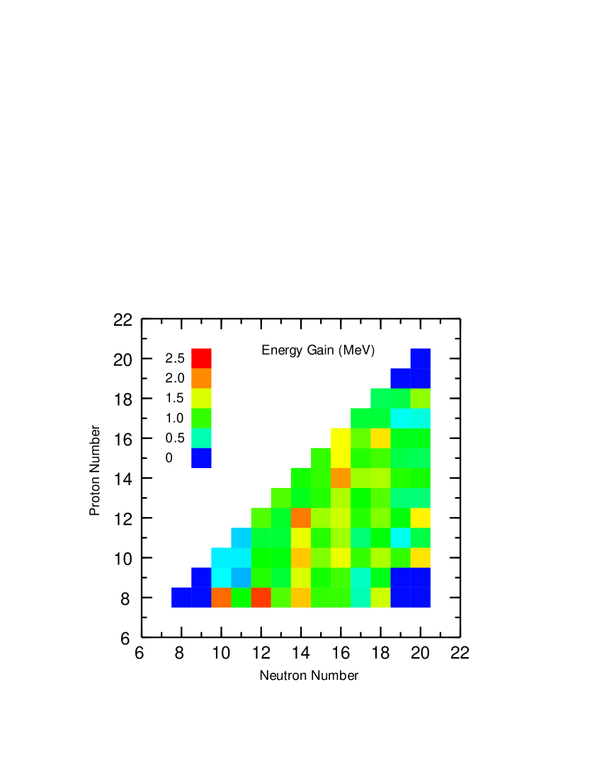
Figure 1: Pairing correlation energy eq. (13) for all $sd$-shell nuclei.

Figure 2: Four selected cuts on the correlation energies displayed in Fig. 1

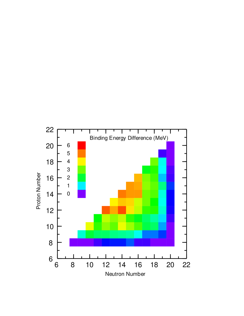
Figure 3: Energy difference between the exact results and our HFP model for all $sd$-shell nuclei.

Figure 4: Energy difference between the exact results and our HFP model for four selected cuts through the $sd$ shell.

III Results

We performed calculations of ground state energies for all nuclei within the $sd$-shell region, from ¹⁷O to ³⁹Ca. Our results table are summarized in Figs. 1-5. In Figs. 1 and 2 we show the energy gain from HFP compared to HF,

$$E_{\rm corr}=E_{\rm HF}-E_{\rm HFP}.$$ (13)

Typical values are one to a few MeV. One observes the well-known odd-even staggering that is characteristic of pairing. In the conventional HFB approach the pairing correlation is zero for many of these nuclei, including cases such as ²⁴O where the spherical shell gap is too large, and cases such as ²⁰Ne, ²⁴Mg and ²⁸Si where the deformed shell gap is too large to support BCS type pairing. The HFP method gives some correlation energy for all $sd$-shell nuclei for which there are at least two active particles ( $9<N<19$ or $9<Z<19$ ). In the practical solution of the equations we find that many $sd$-shell nuclei have two or three energy minima. To have some confidence that we have found the lowest energy solution we start with several initial values of the density matrix including those that are prolate and oblate deformed, spherical and random.

In Figs. 3 and 4 we show the difference between the HFP result and the exact shell-model energy both obtained with the USDB Hamiltonian. For comparison of the methods, the full solution for the ground state of ²⁸Si must take into account 93,710 $M$-scheme Slater determinants. When projected onto good $J=0$ there are 9,216 states, and when projected onto good $J=0,T=0$ there are 839 states. The HFP method requires 92 determinants for protons and 92 for neutrons. The difference is clearly peaked at the $N=Z$ line that can be explained by the proton-neutron pairing being not accounted for in the calculations.

The HFP solution is very close to the exact solution around the edges of the $sd$ shell (see Fig. 4). These nuclei are spherical and the HFP method is equivalent to the spherical exact-pairing method discussed in VBZ01 ; ZV03pairing . The largest deviation from exact is for nuclei near the middle of the $sd$ shell. There are still pairing contributions for deformed nuclei, but the result is different from the naive expectation of just adding ”spherical” contributions. For example, as shown in Fig. 2, the correlation energy is only about 400 keV for the deformed ²⁰Ne, compared to a total of about 3.4 MeV that would be obtained just from adding the 1.7 MeV correlation energies obtained for two neutrons and two protons in a spherical basis (e.g. ¹⁸O and ¹⁸Ne).

Finally in Fig. 5 we show the intrinsic quadrupole moment obtained for the lowest energy solutions for all $sd$-shell nuclei. One observes the well known region of strongly prolate nuclei near ²⁴Mg. ²⁸Si is the most strongly oblately deformed, and there is an island of weak oblate deformation around ³¹Si. It would be interesting to use our $sd$-shell sandbox to clarify the general question of why most nuclei are prolate deformed tajima , by exploring the HFP results with different (but realistic) Hamiltonians.

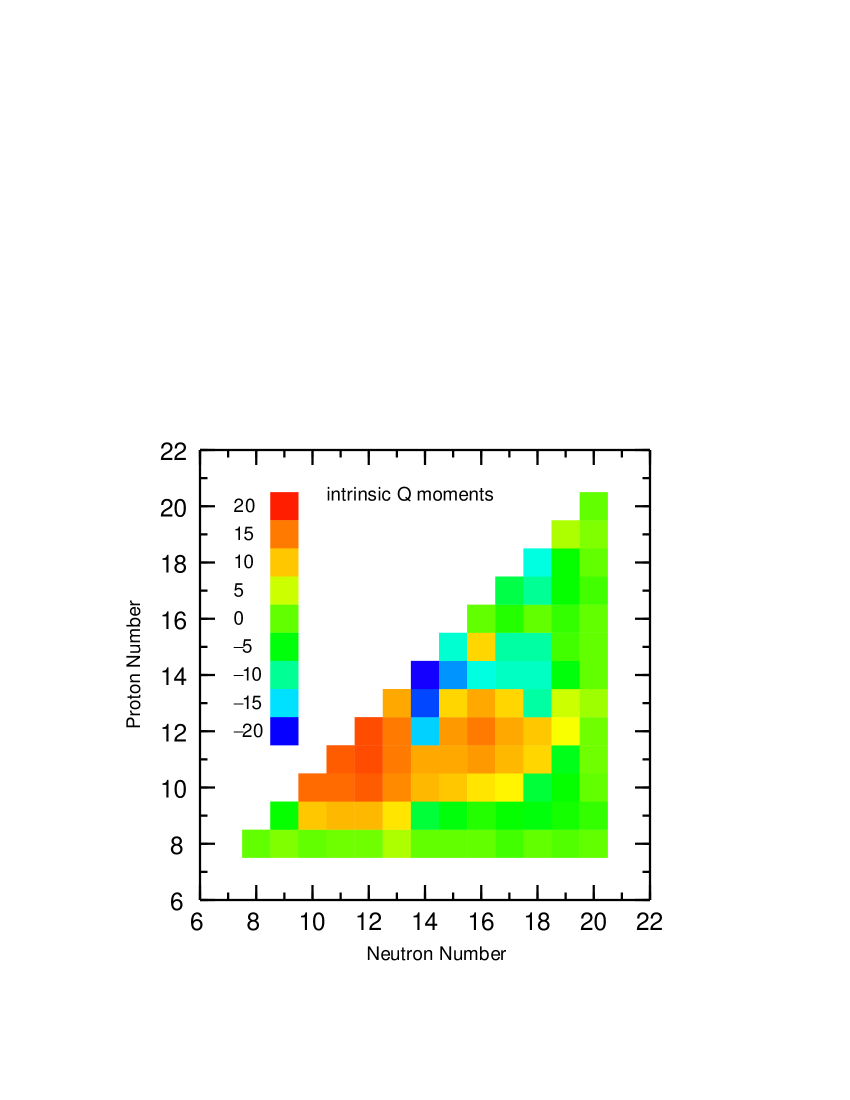
Figure 5: Intrinsic quadrupole moment $Q$, in units $b^{2}$ ($b$ is the oscillator parameter), for the lowest energy configuration for all $sd$-shell nuclei.

IV Conclusion

Obviously, the HFP is still far from adequate away from semi-magic nuclei. The angular momentum non-conservation is certainly a significant deficiency of the wave function, that when repaired will introduce additional correlation energy. There are a number of ways that rotational correlation energies can be calculated, and we are optimistic that HFP wave functions can be used as a better starting point.

Besides rotational energies, proton-neutron pairing effects are omitted in our wave functions. As known martinez99 , such pairing correlations are quite strong close to the $N=Z$ line; they should be included at the next stage of development. Effective Hamiltonians for the HFB solution are explored in rod . Finally, some improvement may follow from including the non-axial configurations with the pairing between more general time-conjugate orbitals (most probably, the mean field in ²⁴Mg is triaxial cole89 ,bender ).

V Acknowledgements

Supported by UNDEF-SciDAC DOE grant DE-FC02-07ER41457 and NSF grants PHY-0555366 and PHY-0758099.

References

- (1) W. Kohn and L.J. Sham, Phys. Rev. 140, A1133 (1965).
- (2) R.M. Dreizler and E.K.U. Gross, Density Functional Theory (Springer, Berlin, 1990).
- (3) A.L. Goodman, Adv. Nucl. Phys. 11, 263 (1979).
- (4) A. Volya, B.A. Brown, and V. Zelevinsky, Phys. Lett. B 509, 37 (2001).
- (5) V. Zelevinsky and A. Volya, Phys. Atom. Nucl. 66, 1829 (2003).
- (6) B.A. Brown and W.A. Richter, Phys. Rev. C 74, 034315 (2006).
- (7) The energies are given in tabular form on http:/unedf.org/hfp/sd.dat.
- (8) N. Tajima and N. Suzuki, Phys. Rev. C 64, 037301 (2001).
- (9) G. Martinez-Pinedo, K. Langanke, and P. Vogel, Nucl. Phys. A651, 379 (1999).
- (10) R. Rodriguez-Guzman, Y. Alhassid and G.F. Bertsch, Phys. Rev. C 77, 064308 (2008).
- (11) B.J. Cole, R.M. Quick, and H.G. Miller, Phys. Rev. C 40, 456 (1989).
- (12) M. Bender and P.H. Heenen, arXiv:0805.4383v1.