Model of Multiphoton Transitions in a Current-Biased Josephson Junction

Abstract

We present a simple model to describe multiphoton transitions between the quasi bound states of a current-driven Josephson junction. The transitions are induced by applying an ac voltage with controllable frequency and amplitude across the junction. The voltage induces transitions across the junction when the frequency $\omega$ satisfies $n\hbar\omega=\Delta E_{10}$, where $\Delta E_{10}$ is the splitting between the ground and first excited quasi-bound state of the junction. We calculate the matrix elements of the transitions as a function of the dc bias current $I$, and the frequency $\omega$ and amplitude $V_{ac}$ of the microwave voltage, for representative junction parameters. We also calculate the frequency-dependent absorption coefficient by solving the relevant Bloch equations when the ac voltage is sufficiently weak. In this regime, the absorption coefficient is a sum of Lorentzian lines centered at the n-photon absorption frequency, of strength proportional to the squared matrix elements. For fixed $V_{ac}$, the transition rate for an $n$-photon process usually decreases with increasing $n$. We also find a characteristic even-odd effect: the absorption coefficient typically increases with $I$ for $n$ even but decreases for $n$ odd. Our results agree qualitatively with recent experiments.

I Introduction

A current-driven Josephson junction can exhibit clear experimental manifestations of quantized energy levelsmartinis1 ; clarke ; martinis2 ; cooper ; makhlin ; silvestrini ; yu . For example, if the junction is biased so that the first minimum of the washboard potential holds only a few quasi-bound states, a suitable ac current can induce transitions between the lowest levels. Population of the excited levels leads to tunneling through the barrier and hence a voltage pulse which can readily be detected experimentally. In part because of this behavior, such junctions are promising candidates for use as qubits (“phase qubits”) in quantum computationmartinis .

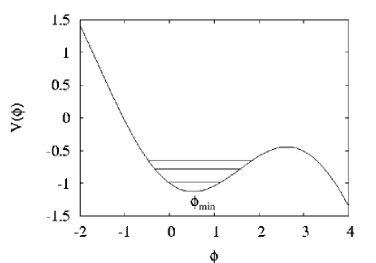
Figure 1: Schematic diagram of the level structure for a Josephson junction subjected to an applied dc current.

Fig. 1 shows a schematic of the level structure for such a junction. Since the potential near a minimum is anharmonic, the level spacings are unequal, as indicated in the sketch. If $\Delta E_{10}=E_{1}-E_{0}$ is the spacing between the ground and first excited state, and $\Delta E_{21}=E_{2}-E_{1}$ is that between the first and second excited level, then $\Delta E_{21}<\Delta E_{10}$. An ac perturbation of frequency $\omega=\Delta E_{10}/\hbar$ will induce transitions between the lowest two states, but because of the anharmonicity, will not produce further excitations to the next level. Rabi oscillations between the lowest two levels have been demonstrated experimentally - that is, the population of the excited level oscillates with a frequency related to the amplitude of the ac pulse, if that perturbation is tuned to be in resonance with $\Delta E_{10}$martinis .

Recently, Wallraff et alwallraff2 have demonstrated multiphoton transitions between the ground and first excited states of a current-biased Josephson junction. In this experiment, transitions were induced between the two levels by subjecting the system to an ac voltage at a frequency $\Delta E_{10}/(n\hbar)$, with $n>1$. Similar transitions have also been observed in flux qubits by Saito et alsaito , and in general in qubits based on anharmonic potentials containing more than two quasi-bound statesdykman . These transitions correspond to absorption of n microwave photons. Such transitions can be used to generate photons at multiples of the incident frequency. If the states involved have a sufficiently long coherence time, the perturbation could also lead to Rabi oscillations arising from multiphoton transitions. Indeed, such Rabi oscillations have been reported experimentallysaito1 . Thus, they could be a significant advance in using these phase qubits in quantum computation.

A number of workers have discussed models for Josephson junctions driven by strong ac perturbations. For example, Ashhab et al.ashhab have considered a two-level system subject to a strong perturbation which is harmonic in time, and demonstrate the occurrence of resonances at frequencies $\omega=\Omega/n$, where $\omega$ is the drive frequency, $\hbar\Omega$ is the unperturbed level splitting, and $n$ is a positive integer. Saito et al.saito1 have observed and analyzed Rabi oscillations corresponding to n-photon transitions in a superconducting flux qubit. Inomata et alinomata have measured and analyzed macroscopic quantum tunneling in intrinsic Bi₂Sr₂CaCu₂O_8+δ Josephson junctions arising from multiphoton transitions, using an analysis based on the classical Josephson junction equation of motion. Koval et al.koval have analyzed the enhancement of Josephson phase diffusion by microwaves, starting from the classical equation for a resistively and capacitively shunted Josephson junction. They obtain a characteristic dependence of the n-photon absorption coeficient on the square of an n^th order Bessel function, similar to that obtained by earlier workersodintsov ; falci , and also resembling that found in the different analysis presented here. Fistul et al.fistul have analyzed the quantum escape of the phase in a strongly driven Josephson junction in the presence of both ac and dc bias curents, in good agreement with their own experiments. Goorden and Wilhelmgoorden analyzed nonlinear driving effects in a continuously driven solid-state qubit using the Bloch-Redfield equation, once again obtaining n-photon resonance effects. Gronbech-Jensen et al.jensen have obtained multiphoton-like effects in Josephson junctions computationally, by solving the classical equation of motion for a junction in the presence of both dc and ac currents. A number of other workers have considered effects of strong ac fields on Josephson junctions in various geometries, mostly in the context of their possible use as qubits for quantum computationstrauch ; berkley ; shnyrkov ; ivlev .

In this paper, we provide a simple model to describe this multiphoton absorption in Josephson phase qubits, using a somewhat different approach from those described above. In our model, we consider a Josephson junction in the presence of a dc driving current plus an ac voltage. The junction is assumed to have very little dissipation, so that the only terms in the Hamiltonian are the Josephson coupling and a capacitive energy. These two combine to produce the well-known pendulum-like Hamiltonian of the junction. The spacing between the levels of this system depends on the current bias.

When the ac voltage is introduced, the gauge-invariant phase difference in the Hamiltonian includes a term arising from that voltage. Use of a Bessel function expansion then shows that this extra term produces $n$-photon transitions between the ground and first excited state of the current-biased junction. We calculate the $n$-photon transition rate as a function of ac voltage amplitude and dc driving current, using the Fermi golden rule. Our model readily produces the transitions seen in experiments.

The remainder of this paper is organized as follows. In the next section, we briefly describe our calculation of the energy eigenvalues and wave functions of the time-independent Hamiltonian. Following this, we describe the expansion which leads to all the n-photon terms in the Hamiltonian. Finally, we present numerical results for the n-photon transition rate, using the Fermi golden rule. A brief discussion follows in Section V.

II Formalism

II.1 Current-Biased Josephson Junction

II.1.1 Hamiltonian

In the absence of resistive shunting, a capacitively shunted Josephson junction driven by a current $I$ can be described by the Hamiltoniantinkham $H=(2en)^{2}/(2C)-\frac{\hbar I_{c}}{2e}\cos\phi-\frac{\hbar I}{2e}\phi$, where $I_{c}$ and $I$ are the junction critical current and the applied current, $\phi$ is the phase difference across the junction, $C$ is the junction capacitance, $n$ is the Cooper pair number difference across the junction, and $2e$ is the charge of a Cooper pair. $n$ and $\phi$ are canonically conjugate operators, satisfying the commutation relation $[n,\phi]=-i$. This relation can be satisfied if we use the representation $n=-i\partial/\partial\phi$ for the number operator. In this representation, $H$ becomes

$$H=-E_{C}\frac{\partial^{2}}{\partial\phi^{2}}-\frac{\hbar I_{c}}{2e}\cos\phi-\frac{\hbar I}{2e}\phi\equiv-E_{C}\frac{\partial^{2}}{\partial\phi^{2}}+U(\phi),$$ (1)

where $E_{C}=2e^{2}/C$ is the charging energy of the junction. Eq. (1) describes a phase ”particle” moving in a ”washboard potential,” $U(\phi)=-\frac{\hbar I_{c}}{2e}\cos\phi-\frac{\hbar I}{2e}\phi$, whose slope is controlled by $I$. In the experiments of Ref. martinis , $E_{C}\ll E_{J}\equiv\hbar I_{c}/(2e)$. Although this regime corresponds to a relatively large junction, it must still be treated quantum-mechanically when the dissipation is very small. For their parameters, the observed quasi-bound state transitions occur when $I/I_{c}\sim 0.99$. In our calculations, for calculational convenience, we have used a larger ratio of $E_{C}/E_{J}$. In order to model the relevant experiments, we solve both the time-independent and the time-dependent Schrödinger equations for the above Hamiltonian, as we now describe.

II.1.2 Solution of the Time-Independent Schrödinger Equation

For $I<I_{c}$, $U(\phi)$ has local potential minima at $\phi=\phi_{k}\equiv\sin^{-1}(I/I_{c})+2\pi k$, $k=0$, $\pm 1$, $\pm 2$,…. For a given $I$, the potential near the first of these minima varies as $U(\phi)\sim U_{min}+K(I)(\phi-\phi_{0})^{2}/2$, where $U_{min}=U(\phi_{0})$ and $K(I)$ is a current-dependent second derivative. If the potential were strictly harmonic near the minimum, the solutions of the time-independent Schrödinger equation would be harmonic oscillator eigenstates, with energies $E_{n}(I)=(n+\frac{1}{2})\hbar\omega_{c}(I)$. These frequencies are readily shown to satisfy

$$\omega_{c}(I)=\omega_{c}(0)\left[1-\frac{I^{2}}{I_{c}^{2}}\right]^{1/4},$$ (2)

where $\omega_{c}(0)=[2eI_{c}/(\hbar C)]^{1/2}$ is the harmonic oscillator frequency at $I=0$, usually called the junction plasma frequency. Because the potential is actually anharmonic, there are two corrections to the above expression for the energies of the eigenstates: the junction levels are not equally spaced as in a harmonic potential, and they are only quasi-bound states, because they can tunnel out of the well.

It is convenient to work with a scaled Hamiltonian

$$\tilde{H}=\frac{H}{E_{J}}=-\cos\phi-\frac{I}{I_{c}}\phi-\frac{E_{C}}{E_{J}}\frac{\partial^{2}}{\partial\phi^{2}}.$$ (3)

The parameters appropriate for the experiments of Ref. martinis are $E_{J}\sim 6.8\times 10^{-14}$ ergs and $E_{C}\sim 8.3\times 10^{-20}$ ergs. In the present calculations, we generally use somewhat different parameters, as discussed below.

To solve the time-independent Schrödinger equation

$$\tilde{H}\Psi_{i}=\tilde{E_{i}}\Psi_{i}$$ (4)

for a given $I/I_{c}$, we first find the local minimum $\phi_{0}=\sin^{-1}(I/I_{c})$ and corresponding potential $\tilde{U}_{min}\equiv\tilde{U}(\phi_{0})$ of the normalized washboard potential $\tilde{U}(\phi)=\cos\phi-\frac{I}{I_{c}}\phi$. We also find the closest local maximum $\phi_{max}$ and the corresponding relative potential maximum, $\tilde{U}_{max}\equiv\tilde{U}(\phi_{max})$. For $I\sim I_{c}$, it is readily shown that the barrier height $\Delta\tilde{U}\equiv\tilde{U}_{max}-\tilde{U}_{min}\propto\left[1-I/I_{c}\right]^{3/2}$. The number of quasi-bound states $N_{b}(I)$ in the well near $\phi=\phi_{0}$ is approximately $N_{b}(I)\sim\Delta U(I)/[\hbar\omega_{c}(I)]$. The lifetime of a given quasi-bound state in the well is also determined by this ratio.

To find the quasi-bound states, we expand the solutions of eq. (4) in the set of harmonic oscillator states corresponding to the local minimum of $U(\phi)$ for the given $I/I_{c}$ cleland . These take the form

$$\psi_{n}(\phi)=2^{-n/2}(n!)^{-1/2}\bigg{(}\frac{1}{(\Delta\phi)^{2}\pi}\bigg{)}^{1/4}\times$$ (5)

$$\times\exp\bigg{(}-\frac{(\phi-\phi_{0})^{2}}{2(\Delta\phi)^{2}}\bigg{)}H_{n}\bigg{(}\frac{\phi-\phi_{0}}{\Delta\phi}\bigg{)},$$

where $H_{n}(\xi)$ is a Hermite polynomial, and

$$(\Delta\phi)^{2}=[2e^{2}/\hbar C][\hbar C/(2eI_{c})]^{1/2}\left(1-\frac{I^{2}}{I_{c}^{2}}\right)^{-1/4}.$$ (6)

In this form, the orthonormal states are harmonic oscillator eigenstates of the Hamiltonian

$${H}_{harm}(I)=U_{min}+\frac{\hbar I_{c}}{2e}\left(1-\frac{I^{2}}{I_{c}^{2}}\right)^{1/2}\times$$ (7)

$$\times\frac{(\phi-\phi_{0})^{2}}{2}-E_{C}\frac{\partial^{2}}{\partial\phi^{2}},$$

where we have used the relation (2).

The solution $\Psi_{i}(\phi)$ of the time-independent Schrödinger equation is then expressed as $\Psi_{i}(\phi)=\sum_{n}a_{n}\psi_{n}(\phi)$. In matrix form, the Schrödinger equation becomes

$$\sum_{n}(\tilde{H}_{mn})a_{n}=\tilde{E}_{i}a_{m},$$ (8)

where $\tilde{H}_{mn}=\int_{-\infty}^{\infty}\psi_{m}(\phi)\tilde{H}\psi_{n}(\phi)d\phi$. In our calculations, we include as many as the first $23$ harmonic oscillator states in our matrix. As a check of our procedure, we have calculated the lowest three energy eigenvalues $E_{0}$, $E_{1}$, and $E_{2}$, and corresponding wave functions, for $I/I_{c}=0.99$, approximately the dc current studied in Ref. martinis , using their quoted values of $E_{C}$ and $E_{J}$, and from these compute $\Delta E_{10}$, $\Delta E_{21}$ and the ratio $\Delta E_{21}/\Delta E_{10}$. We find $\Delta E_{10}=3.86\times 10^{-17}$ erg, quite close to the value of $4.51\times 10^{-17}$ erg measured in Ref.  martinis . The difference may arise because the actual values of $I/I_{c}$ and $C$ in the junction studied experimentally differ slightly from the quoted experimental values. We also calculate $\Delta E_{21}/\Delta E_{10}=0.928$, quite close to the value of 0.9 quoted for this quantity in Ref. martinis .

Once we have these eigenstates, we determine how many of these are ”quasi-bound” by finding out how many satisfy $\tilde{E}_{n}<\tilde{U}_{max}$. In general, we have considered only values of $I/I_{c}$ such that there are at least three quasi-bound states. For the parameters of Ref. martinis , this condition is satisfied up to $I/I_{c}\approx 0.99$.

II.2 Current-Biased Josephson Junction with AC Voltage

In the presence of an ac voltage $V_{ac}\sin\omega t$, the proper gauge-invariant phase difference takes the formtinkham : $\phi\rightarrow\phi+\frac{2eV_{ac}}{\hbar\omega}\cos{\omega t}$. The correspondingly modified Hamiltonian is $H=-E_{c}\frac{\partial^{2}}{\partial\phi^{2}}-\frac{\hbar I}{2\,e}\phi-\frac{\hbar I_{c}}{2\,e}\cos\left[\phi+\frac{2eV_{ac}}{\hbar\omega}\cos\omega t\right]-\frac{V_{ac}I}{\omega}\cos\omega t$. This formulation makes clear that the effects of the ac voltage are characterized by the frequency $\omega$ and by the dimensionless variable $z=2eV_{ac}/(\hbar\omega)$. In the dimensionless form of Section IIA, the Hamiltonian takes the form

$$\tilde{H}=-\frac{E_{C}}{E_{J}}\frac{\partial^{2}}{\partial\phi^{2}}-\frac{I}{I_{c}}\phi-\cos\left[\phi+\frac{\tilde{V}_{ac}}{\tilde{\omega}}\cos(\tilde{\omega}\tau)\right]$$

$$-\frac{\tilde{V}_{ac}}{\tilde{\omega}}\frac{I}{I_{c}}\cos(\tilde{\omega}\tau),$$ (9)

where we have introduced the dimensionless frequency $\tilde{\omega}=\frac{2e\omega}{I_{c}}$, dimensionless time $\tau=\frac{I_{c}t}{2e}$, and dimensionless ac voltage amplitude $\tilde{V}_{ac}=\frac{V_{ac}}{R_{0}I_{c}}$, where $R_{0}=\hbar/(4e^{2})$.

We are interested in terms in this Hamiltonian which will induce transitions between the quasi-bound states discussed in Section IIA. Since the last term in eq. (II.2) is a c-number, it will not induce such transitions. The only relevant term is the Josephson energy $\cos\left[\phi+\frac{\tilde{V}_{ac}}{\tilde{\omega}}\cos(\tilde{\omega}\tau)\right]$. To extract the multiphoton transitions, we may express this energy in terms of Bessel functions using the expansions abram $\cos(z\cos(\theta))=J_{0}(z)+2\sum_{k=1}^{\infty}(-)^{k}J_{2k}(z)\cos(2k\theta)$ and $\sin(z\cos(\theta))=2\sum_{k=0}^{\infty}(-)^{k}J_{2k+1}(z)\cos{(2k+1)\theta}$. Writing $z=\tilde{V}_{ac}/\tilde{\omega}$ and $\theta=\tilde{\omega}\tau$, and using a trigonometric identity, we can easily show that

$$\cos(\phi+\frac{\tilde{V}_{ac}}{\tilde{\omega}}\cos(\tilde{\omega}\tau))=J_{0}\bigg{(}\frac{\tilde{V}_{ac}}{\tilde{\omega}}\bigg{)}\cos\phi$$

$$+2\sum_{n=1}^{\infty}J_{n}\bigg{(}\frac{\tilde{V}_{ac}}{\tilde{\omega}}\bigg{)}\cos(\phi+n\pi/2)\cos(n\tilde{\omega}\tau).$$ (10)

Thus, in the presence of an ac voltage, the potential energy term in the Schrödinger equation is modified in two ways: (i) the strength of the dc part is reduced by a factor of $J_{0}(\tilde{V}_{ac}/\tilde{\omega})$, and (ii) there are an infinite series of additional ac terms at frequencies $\tilde{\omega}$ and all its harmonics. These harmonic terms will induce the multiphoton transitions. Given these approximations, the full Hamiltonian takes the form $H=H_{0}+H_{1}$, where

$$H_{0}=-E_{c}\frac{\partial^{2}}{\partial\phi^{2}}-\frac{\hbar I}{2e}\phi-\frac{\hbar I_{c}}{2e}J_{0}\left(\frac{2eV_{ac}}{\hbar\omega}\right)\cos\phi$$ (11)

and

$$H_{1}=2\frac{\hbar I_{c}}{2e}\sum_{n=1}^{\infty}J_{n}\left(\frac{2eV_{ac}}{\hbar\omega}\right)\cos(\phi+n\pi/2)\cos(n\omega t).$$ (12)

The condition for the occurrence of an $n$-photon transition between the ground and first excited state of the current-driven junction is

$$\Delta E_{10}(I,V_{ac},\omega)=n\hbar\omega.$$ (13)

Here $\Delta E_{10}(I,V_{ac},\omega)$ is the energy splitting between the ground and first excited state when the ac voltage amplitude and frequency are $V_{ac}$ and $\omega$. We solve eq. (13) by a self-consistent procedure. For a given $V_{ac}$ and $\omega$, the junction levels are obtained as solutions of the time-independent Schrödinger equation $H(V_{ac},\omega)\Psi=E\Psi$, where $H(V_{ac},\omega)$ is given by eq. (2) but with $E_{J}$ replaced by $E_{J}J_{0}[2eV_{ac}/(\hbar\omega)]$ To find the strength of the $n$-photon transitions, we make an initial guess for $\omega$, solve the dc Schrödinger equation using the potential $-E_{J}[J_{0}(2eV_{ac}/(\hbar\omega)]\cos\phi$, and iterate until eq. (13) is satisfied. As in the previous section, we expand the quasi-bound eigenstates as a linear combination of harmonic oscillator wave functions. Thus, we make an initial guess for $\omega$, calculate the eigenvalues, and then change $\omega$ such that $n\hbar\omega=\Delta E_{10}(I,V_{ac},\omega)$. The eigenvalues are recalculated using this new $\omega$, and the procedure is repeated until the energy levels remain unchanged to within an absolute error of $1.0\times 10^{-4}E_{J}$. Although eq. (II.2) is valid, in principle, for any value of $z$, this procedure is not reasonable unless the strength of the potential $[\hbar I_{c}/(2e)]J_{0}[2eV_{ac}/(\hbar\omega)]>0$. In practice, we find that, for our choice of parameters (see below), our procedure leads to two or more bound states in the well only if $\frac{2\,eV_{ac}}{\hbar\omega}<0.58$.

Given the energy levels, the n-photon transition rate can be calculated, in principle, from the Fermi Golden Rulemerzbach :

$$\tilde{\Gamma}_{n}(I,V_{ac},\omega) = \frac{2\pi}{\hbar}|\langle 0|V_{n}|1\rangle|^{2}\delta(E_{s}-n\hbar\omega)$$ (14)

$$\equiv \Gamma_{n}(I,V_{ac},\omega)\delta(\Delta E_{10}-n\hbar\omega),$$

where the perturbing potential for n-photon transitions is $V_{n}=2J_{n}(\frac{2\,e\,V_{ac}}{\hbar\omega})\cos(\phi+n\pi/2)$. The states $\langle 0|$ and $|1\rangle$ are the ground and first excited states of the current-biased junction in the presence of microwave radiation.

Eq. (14) is suitable for describing transitions between bound states with sharply defined energies. In reality, as already noted, the states of interest are only quasi-bound, since, for both the initial and the final state, the phase “particle” can tunnel out through the barrier of the washboard potential. One way to take account of this tunneling is to describe both the initial and the final states by complex energies $E_{0}+i\gamma_{0}$ and $E_{1}+i\gamma_{1}$. The quantities $\gamma_{0}/\hbar$ and $\gamma_{1}/\hbar$ then represent the tunneling rates out of the states $|0\rangle$ and $|1\rangle$. If this description is used, the n-photon transition rate is described by the second form of the Fermi Golden Rulemerzbach , which represents the transition rate from an initial state of energy $E_{0}$ into a continuum of final states:

$$\tilde{\Gamma}_{n}(I,V_{ac},\omega)=\frac{2\pi}{\hbar}|\langle 0|V_{n}|1\rangle|^{2}\rho(\Delta E_{10}-n\hbar\omega).$$ (15)

Here $\rho(E)$ is the density of final states. If the final state is approximated by a complex energy $E_{1}+i\gamma_{1}$, then the quantity which replaces the delta function in eq. (14) is

$$\rho(\Delta E_{10}-n\hbar\omega)=\frac{1}{\pi}\frac{\gamma_{1}}{(\Delta E_{10}-n\hbar\omega)^{2}+\gamma_{1}^{2}},$$ (16)

where the normalization is chosen so that $\int_{-\infty}^{\infty}\rho(E)dE=1$. The corresponding rate of energy absorption is then

$$\alpha=\sum_{n}n\hbar\omega\tilde{\Gamma}_{n}(I,V_{ac},\omega)(n\hbar\omega),$$ (17)

where the factor of $n\hbar\omega$ denotes the fact that the energy absorbed in an n-photon transition is $n\hbar\omega$.

In order to use this formulation, we need to determine the width $\gamma_{1}$. For the regime studied in typical experiments, it should be sufficient to treat $\gamma_{1}$ within the WKB approximation. This approximation gives

$$\gamma_{1}\sim\hbar\omega_{0}\exp\left(-2S/\hbar\right),$$ (18)

where $\omega_{0}$ is a suitable attempt frequency for escaping the well, and S is the WKB action. In this case, $S(E)=\int_{\phi_{i}}^{\phi_{f}}p_{\phi}d\phi$, where $p_{\phi}=-i\hbar(\partial/\partial\phi)$ is the momentum canonically conjugate to $\phi$, and $\phi_{i}$ and $\phi_{f}$ are the values of $\phi$ at the left and right hand edges of the tunneling barrier. From the Hamiltonian (1) of the current-driven Josephson junction, we replace $p_{\phi}$ in the WKB approximation by $\hbar\sqrt{[E-U(\phi)]/E_{C}}$. Thus, we finally obtain (setting $E=E_{1}$ for the final state)

$$\frac{S(E)}{\hbar}\sim\int_{\phi_{i}}^{\phi_{f}}\sqrt{\frac{E-U(\phi)}{E_{C}}}d\phi,$$ (19)

where $\phi_{i}$ and $\phi_{f}$ are determined by $U(\phi_{i})=U(\phi_{f})=E_{1}$. We give some numerical estimates of $\gamma_{1}$, and of the corresponding multiphoton absorption, at the end of Section IV.

Besides the escape rate from the metastable potential well, another source of line broadening is dissipation due to the finite shunt resistance $R$ of the underdamped Josephson junction. We expect that this dissipation will give rise to another contribution to $\gamma_{1}$, thereby further increasing the linewidths of the multiphoton absorption lines. The magnitude of this contribution obviously depends on the magnitude of $R$.

III Inclusion of Dissipation using Bloch Equations

The form of the result (17) for multiphoton absorption in the presence of dissipative processes can also be obtained using the analog of the Bloch equations familiar in NMR. In this section, we describe this method. Related approaches have been discussed, e. g., by Shevchenko et alshevchenko . Our approach goes beyond their work because we directly compute the necessary matrix elements and thus obtain explicit expressions for the absorption coefficient.

We again consider the Hamiltonian $H=H_{0}+H_{1}$ of eqs. (11) and (12), and consider transitions only between the lowest two states of the Hamiltonian (11). Since we are considering only two states, we may write the Hamiltonian (11) in operator form as $H_{0}=-\frac{\Delta E_{10}}{2}\sigma_{z}+\mathrm{const}$, where $\Delta E_{10}(I,V_{ac},\omega)$ denotes the splitting between the lowest two energy levels in the presence of an ac voltage of amplitude $V_{ac}$ and frequency $\omega$. The last term is a constant which can be chosen to vanish by proper selection of the energy zero. we choose our zero of energy so that this constant vanishes. $\sigma_{i}$ ($i=x$, $y$, $z$) are the three standard Pauli matrices. If we retain only that part of $H_{1}$ which produces transitions between $|0\rangle$ and $|1\rangle$, then the time-dependent perturbation (12) can be written

$$H_{1}=\sum_{n=1}^{\infty}2J_{n}\left(\frac{2eV_{ac}}{\hbar\omega}\right)\langle 0|\cos(\phi+n\pi/2)|1\rangle\cos(n\omega t)\sigma_{x}.$$ (20)

In writing the Hamiltonian in this form, we are not only considering just two levels but also are using the fact that the diagonal matrix elements of the form $\langle 0|H_{1}(t)|0\rangle$ and $\langle 1|H_{1}(t)|1\rangle$ vanish.

In the absence of relaxation processes, the Heisenberg equations of motion can be used to obtain equations of motion for expectation values of any operators. We write the time-dependent wave function as $|\psi(t)\rangle=a(t)|0\rangle+b(t)|1\rangle$, where $|a|^{2}+|b|^{2}=1$. We also write the Hamiltonian as $H=H_{0}+H_{1}=-{\bf B}\cdot{\bf\sigma}/2$, where ${\bf\sigma}$ is the ordered triple of Pauli matrices, and ${\bf B}$ is an effective magnetic field, which is the sum of a time-independent $B_{z}{\bf\hat{z}}$ and a time-dependent part $B_{x}(t){\bf\hat{x}}$, with

$$B_{z}=\Delta E_{10},$$ (21)

$$B_{x}(t)=\frac{\hbar I_{c}}{2e}\sum_{n=1}^{\infty}4J_{n}\left(\frac{2eV_{ac}}{\hbar\omega}\right)\langle 0|\cos(\phi+n\pi/2)|1\rangle\cos(n\omega t),$$ (22)

and $B_{y}=0$.

The Heisenberg equations of motion for the expectation value of any operator ${\cal O}$ are $i\hbar\frac{d}{dt}\langle{\cal O}\rangle=i\hbar\frac{d}{dt}\langle\psi|{\cal O}|\psi\rangle=\langle\psi|[{\cal O},H]|\psi\rangle$. For the present Hamiltonian $H=H_{0}+H_{1}$, including only the two lowest energy levels, they reduce to the well-known form

$$\frac{d}{dt}{\bf M}=\frac{1}{\hbar}{\bf M}\times{\bf B},$$ (23)

where ${\bf M}=\langle{\bf\sigma}\rangle$, the brackets denoting a quantum-mechanical expectation value.

The form of eq. (23) suggests that, to include dissipative processes, we should generalize this equation so that it has the same form as the Bloch equations of magnetic resonance:

$$\frac{d}{dt}{\bf M}_{\perp} = \frac{1}{\hbar}\left({\bf M}\times{\bf B}\right)_{\perp}-\frac{{\bf M}_{\perp}}{\tau_{\phi}}$$

$$\frac{d}{dt}M_{z} = \frac{1}{\hbar}\left({\bf M}\times{\bf B}\right)_{z}-\frac{(M_{z}-M_{0})}{\tau_{r}}.$$ (24)

Here $\tau_{\phi}$ and $\tau_{r}$ are relaxation times analogous to $T_{1}$ and $T_{2}$ in magnetic resonance theory, ${\bf M}_{\perp}\equiv(M_{x},M_{y})$, and $M_{0}\hat{z}$ is the equilibrium value of $\langle\sigma\rangle$ to which ${\bf M}$ reverts when the time-dependent perturbation is turned off [see, e. g., Ref. slichter ).

Given the solution for ${\bf M}(t)$, we can calculate the absorbed power by adapting a standard approach used in NMR calculationsslichter , namely, we solve for $M_{x}(t)$ in the limit when $B_{x}(t)$ is weak. In this regime, $M_{x}(t)$ can be obtained in closed form by superimposing the solutions arising from each separate frequency $\Omega$ of $B_{x}(t)$ in eq. (22). For small $B_{x}$, $M_{z}\sim M_{0}$ through first order in $B_{x}$ Writing the three Bloch equations in component form, and also assuming that both $M_{x}$ and $M_{y}$ vary with time as $\exp(-i\Omega t)$, we obtain

$$-i\Omega M_{x} = \frac{1}{\hbar}M_{y}B_{z}-\frac{M_{x}}{\tau_{\phi}};$$

$$-i\Omega M_{y} = \frac{1}{\hbar}(M_{0}B_{x}-M_{x}B_{z})-\frac{M_{y}}{\tau_{\phi}}.$$ (25)

The resulting solution for $M_{+}\equiv M_{x}+iM_{y}$ is readily found to be

$$M_{+}(t)=\frac{(B_{x}/\hbar)M_{0}e^{-i\Omega t}}{(B_{z}/\hbar)-\Omega-i/\tau_{\phi}}.$$ (26)

For the present problem, the transverse field is a sum of terms of the form $B_{nx}\cos(n\omega t)\equiv(B_{nx}/2)(e^{-i\omega t}+e^{+i\omega t})$, which induces a transverse magnetization

$$M_{n,+}(t) = (B_{nx}/2\hbar)M_{0}\times$$

$$\times \left(\frac{e^{-in\omega t}}{B_{nz}/\hbar-n\omega-i/\tau_{\phi}}+\frac{e^{in\omega t}}{B_{z}/\hbar+n\omega-i/\tau_{\phi}}\right).$$

Hence $M_{nx}(t)\equiv\mathrm{Re}M_{n,+}(t)$ satisfies

$$\frac{2\hbar M_{0}M_{n,x}}{B_{nx}}=$$

$$\frac{\cos(n\omega t)(B_{nx}/\hbar-n\omega)+\sin(n\omega t)(1/\tau_{\phi})}{(B_{z}/\hbar-n\omega)^{2}+1/\tau_{\phi}^{2}}$$

$$+\frac{\cos(n\omega t)(B_{nx}/\hbar+n\omega)-\sin(n\omega t)(1/\tau_{\phi})}{(B_{z}/\hbar+n\omega)^{2}+1/\tau_{\phi}^{2}}.$$ (28)

Finally, the total absorption can be written

$$\alpha=\langle\frac{d}{dt}\langle H_{1}(t)\rangle\rangle_{t}$$ (29)

where the outer brackets denote a time average. For our time-dependent perturbation, this expression is readily shown to be equivalent to

$$\alpha=\sum_{n=1}^{\infty}M_{0}\left(\frac{B_{nx}}{\hbar}\right)^{2}\frac{n\omega}{4\tau_{\phi}}\times$$

$$\times\left[\frac{1}{(B_{z}/\hbar-n\omega)^{2}+1/\tau_{\phi}^{2}}+\frac{1}{(B_{z}/\hbar+n\omega)^{2}+1/\tau_{\phi}^{2}}\right].$$ (30)

In terms of the parameters of the two-level system, we have

$$\alpha=\sum_{n=1}^{\infty}\alpha_{n},$$ (31)

where

$$\alpha_{n}=M_{0}\frac{\hbar I_{c}^{2}}{2e^{2}}J_{n}\left(\frac{2eV_{ac}}{\hbar\omega}\right)^{2}\frac{n\omega}{4\tau_{\phi}}|\langle 0|\cos(\phi+n\pi/2)|1\rangle|^{2}{\cal L}(n\omega),$$ (32)

where ${\cal L}(n\omega)$ is a Lorentzian given by

$${\cal L}(n\omega)=\frac{1}{(\Delta E_{10}/\hbar-n\omega)^{2}+1/\tau_{\phi}^{2}}$$

$$+\frac{1}{(\Delta E_{10}/\hbar+n\omega)^{2}+1/\tau_{\phi}^{2}}.$$ (33)

Thus, in this approximation, the total absorption is just a sum of Lorentzians. The quantity $M_{0}$, undetermined in this calculation, is given by $2p-1$, where $p$ is the probability that the junction is to be found in the lower of the two states, $|0\rangle$. The integrated strength of the n-photon absorption line is

$$\int_{-\infty}^{\infty}\alpha_{n}(\omega)=M_{0}\frac{2\pi}{\hbar}\tau_{\phi}B_{nx}^{2}B_{nz}=\Gamma_{n}.$$ (34)

where $\Gamma_{n}$ is the coefficient of eq. (14). Eqs. (31), (32), and (33) are basically equivalent to the result (17) obtained in the previous section. The quantity $\hbar/\tau_{\phi}$ is analogous to the quantity $\gamma_{1}$ in eq. (16).

In principle, a more accurate solution could be obtained by solving the Bloch equations directly for the full time-dependent Hamiltonian arising from the microwave voltage. This would lead to a more complicated absorption lineshape, which would probably depend on $\tau_{r}$ as well as $\tau_{\phi}$.

IV Numerical Results

We now describe our calculated $n$-photon transition rates $\Gamma_{n}(I,V_{ac},\omega)$, in the absence of dissipation, for $n$ ranging from $1$ to $5$. In each calculation, we start by choosing $I$, $V_{ac}$ and $n$. The frequency and energy-level splitting are then determined self-consistently, as described above, and the transition rate $\Gamma_{n}$ is calculated [see eq. (14)]. In all calculations, we choose $E_{C}=8.53\times 10^{-18}$ erg, $E_{J}=6.91\times 10^{-14}$ erg, and hence $E_{C}/E_{J}=1.235\times 10^{-4}$. For this choice, there are three quasi-bound states at $I/I_{c}\sim 0.85$, and the ratio $\Delta E_{21}/\Delta E_{10}\sim 0.928$.

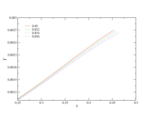
Figure 2: (Color online.) Single photon transition rate $\Gamma_{1}$ (in units of $E_{J}^{2}/\hbar$) as a function of $z=\frac{2eV_{ac}}{\hbar\omega}$ for currents ranging from $I/I_{c}=0.85$ to $0.856$. The red (dark gray full) line, green (light gray dashed) line, blue (gray dotted) line, and violet (gray dash-dotted) line correspond to z = 0.85, 0.852, 0.854, and 0.856 respectively. The same color and grayscale codes are used in Figs. 3-11.

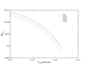
Figure 3: (Color online.) Energy level splitting $\Delta E_{10}$ (in units of $E_{J}$ )between the ground and first excited states as a function of $V_{ac}$ for currents $I/I_{c}$ ranging from $0.85$ to $0.856$ for the self-consistently determined frequency $\omega=\Delta E_{10}/\hbar$. Parameters are the same as in Fig. 2.

In Fig. 2, we show $\Gamma_{1}$ as a function of $z=2eV_{ac}/(\hbar\omega)$ for a narrow range of driving currents, $0.85<I/I_{c}<0.856$. The frequency is chosen so that $\hbar\omega=\Delta E_{10}(I,V_{ac},\hbar\omega)$. For the chosen range of $I$, $\Gamma_{1}$ is quite insensitive to $I$. In Fig. 3, we plot $\Delta E_{10}(I,V_{ac},\omega)$ as a function of $V_{ac}$ at a frequency satisfying $\hbar\omega=\Delta E_{10}$. The splitting decreases roughly quadratically with increasing $V_{ac}$. This behavior is expected from the Bessel-function dependence of the potential strength, since $J_{0}(z)$ decreases approximately quadratically with $z$, resulting in a shallower potential well with increasing $z$ for fixed $I$.

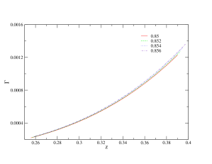
Figure 4: (Color online.) Two photon transition rate $\Gamma_{2}$ plotted as a function of $z=\frac{2eV_{ac}}{\hbar\omega}$ for currents ranging from $I/I_{c}=0.85$ to $0.856$ and the self-consistently determined frequency $\omega=\Delta E_{10}/(2\hbar)$.

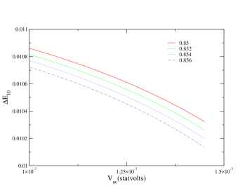
Figure 5: (Color online.) Energy level splitting $\Delta E_{10}$ as a function of $V_{ac}$ for currents ranging $I/I_{c}=0.85$ to $0.856$ and a frequency such that $\omega=\Delta E_{10}/(2\hbar)$.

In Figs. 4 and 5, we show corresponding results for two-photon transitions (n = 2), all other parameters being kept the same as in Figs. 2 and 3. In these plots, we have considered smaller values of $V_{ac}$ than for $n=1$. We do so because of the condition $n\hbar\omega=\Delta E_{10}(I,V_{ac},\omega)$ which must be satisfied for $n$-photon absorption. Two-photon absorption thus occurs at roughly half the frequency of one-photon absorption, as expected. $\Delta E_{10}$ is more sensitive to $V_{ac}$ at such frequencies than it would be for one-photon absorption. We must also keep $V_{ac}$ well below the limit $V_{ac}=0.58n\hbar\omega/(2e)$, above which there are no quasi-bound states.

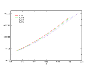
Figure 6: (Color online.) Same as Fig. 4 but for the three-photon transition rate $\Gamma_{3}$.

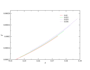
Figure 8: (Color online.) Same as Fig. 4 but for four-photon transitions

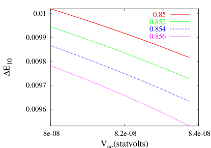
Figure 9: (Color online.) Same as Fig. 5 but for four-photon transitions.

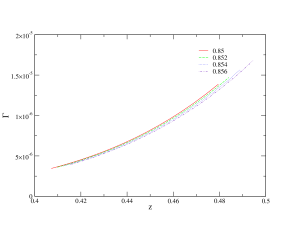
Figure 10: (Color online.) Same as Fig. 4 but for five-photon transitions.

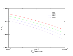
Figure 11: (Color online.) Same as Fig. 5 but for five-photon transitions.

The corresponding results for three-photon transitions are shown in Figs. 6 and 7. In general $\Gamma_{3}<\Gamma_{1}$, as expected, since the corresponding matrix element involves $J_{3}(z)$ instead of $J_{1}(z)$. Furthermore, of course, for a given $I$ and $V_{ac}$, the frequency required to produce the $n=3$ transition is smaller than that for $n=1$. We have also considered smaller values of $V_{ac}$ than for $n=1$, because the sensitivity of $\Delta E_{10}$ to $V_{ac}$ is greater for $n=3$ than for $n=1$. In Figs. 8 -11 we show the corresponding results for $n=4$ and $n=5$ transitions.

All the above results make clear a noticeable difference between even and odd transitions: for $n$ even, $\Gamma_{n}$ increases with increasing $I$ at fixed $z$, whereas for $n$ odd, $\Gamma_{n}$ decreases with increasing $I$. (We have not considered a very large range of $I$ in calculating these rates.) This difference is easily understood from the matrix elements of the time-dependent perturbation which enter equation (14) for the transition rate. Specifically, the argument of the cosine term has a phase shift of $n\pi/2$, so that the perturbing potential varies as $\sin\phi$ for odd $n$. Because the perturbation is even in $\phi$ for even $n$, $\Gamma_{n}$ vanishes for even $n$ at $I=0$, and hence should increase within increasing $I$, as we observe. By contrast, the perturbation is odd in $\phi$ for odd $n$, so that $\Gamma_{n}$ for odd $n$ is finite at $I=0$ but decreases with increasing $I$. Thus, we interpret this even-odd effect as arising from the different parities of the time-dependent perturbation for $n$ even and $n$ odd.

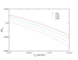
Figure 7: (Color online.) Same as Fig. 5 but for three-photon transitions.

Figs. 2 - 10 also show that, for fixed $z=2eV_{ac}/(\hbar\omega)$ and fixed $I/I_{c}$, $\Gamma_{n}$ generally decreases with increasing $n$. Comparison of the behavior for different $n$ is somewhat difficult, because the relevant value of the parameter $z=2eV_{ac}/(\hbar\omega)$ is different for each $n$. This behavior is consistent with that observed in the experiments of Ref. martinis . These authors find that, when the first excited state is populated by $n$-photon transitions, the apparent lifetime increases with increasing $n$. This increased lifetime is simply the consequence of a smaller transition rate for the higher-$n$ transitions.

Finally, we estimate how these n-photon transition rates are affected when we include reasonable estimates of level broadening due to tunneling of the phase “particle” through the barrier. We use the formalism of eqs. (15) - (19). Using the values of $E_{C}$ and $E_{J}$ given above (which lead to $E_{C}/E_{J}=1.235\times 10^{-4}$), we obtain estimates for $\exp[-2S(E_{1})/\hbar]$ given in Table 1 for $I/I_{c}=0.85$, $0.90$, and $0.95$. The corresponding width $\gamma_{1}$ of the Lorentzian line shape is given, as a fraction of $\hbar\omega_{c}(I)$, in the last column. In calculating $S(E_{1})$, we have estimated $E_{1}$, the energy of the second-lowest quasibound state, by expanding the potential in the Hamiltonian (1) through third order in $\phi-\phi_{0}$, and have included the cubic term as a perturbation to the resulting harmonic Hamiltonian, through second order in perturbation theory. The resulting values of $E_{1}$ are also shown in the Table.

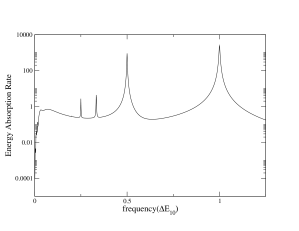
Figure 12: Plot of the absorption spectrum $\tilde{\Gamma}_{tot}(I,V_{ac},\omega)=\sum_{n=1}^{nmax}\tilde{\Gamma}_{n}(I,V_{ac},\omega)$ (in units of $\Delta E_{10}/\hbar$) as a function of $\omega$, for $I/I_{c}=0.95$ and ac amplitude given by $2eV_{ac}/(\Delta E_{10})=0.2$, as calculated using the parameters and method described in the text.

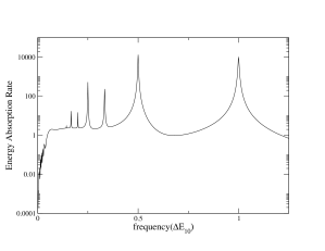
Figure 13: Same as Fig. 12, but with ac amplitude given by $2eV_{ac}/(\Delta E_{10})=0.4$.

In order to illustrate a typical multiphoton absorption spectrum in the presence of this dissipation, we have carried out a simplified model calculation of the total absorption spectrum, $\tilde{\Gamma}_{tot}(I,V_{ac},\omega)=\sum_{n=1}^{n_{max}}\tilde{\Gamma}_{n}(I,V_{ac},\omega)$, where $\tilde{\Gamma}_{n}$ is given by eqs. (15) and (16). The results are shown in Figs. 12 and Fig. 13 for $I/I_{c}=0.95$, $E_{C}=8.53\times 10^{-18}$ erg, and $E_{J}=6.91\times 10^{-14}$ erg as earlier in this paper. We assumed $I/I_{c}=0.95$ and considered two ac amplitudes given by $2eV_{ac}/\hbar\omega_{0}(I)=0.2$ and $0.4$. We have included all multiphoton terms through $n_{max}=7$. For this calculation, we have calculated both the energies $E_{0}$ and $E_{1}$ and the matrix elements $\langle 0|V_{n}|1\rangle$ by including only the lowest order anharmonic corrections to $E_{0}$, $E_{1}$, $|0\rangle$ and $|1\rangle$, the perturbation being the terms in the potential of third order in $\phi-\phi_{0}$. In the interests of simplifying this calculation, we have also neglected the dependence of the Josephson well depth on the ratio $z=2eV_{ac}/(\hbar\omega)$ [eq. (11)]. In practice, this means that this model calculation becomes increasingly inaccurate at low frequencies. For our choice of $V_{ac}$, this dependence on $V_{ac}$ should probably be included for $\hbar\omega<0.2\Delta E_{10}$. With these assumptions, however, both the energies and the matrix elements can be computed in closed form in terms of $E_{J}$, $E_{C}$ and $I/I_{c}$. The results show that the strength of the lines falls off rapidly with increasing $n$ for our chosen value of $V_{ac}$.

In these calculations, and with our estimate of $\gamma_{1}$, we have not included the effects of the shunt resistance $R$, which is always present in a realistic Josephson junction. This shunt resistance will further broaden the multiphoton absorption spectrum, but is distinct from the tunneling through the barrier treated above. For the junctions studied in Ref. wallraff2 , $1/[\omega_{p}(0)\tau]<5\times 10^{-4}$, using their parameters of critical current density $j=1.1$ kA/cm², junction area $\sim(5.5\mu)^{2}$, $C\sim 1.6$ pF, and shunt resistance $R>500\Omega$. Here $\tau=RC$ is the relaxation time associated with resistive dissipation within the junction. If we assume the same value of $1/[\omega_{p}(0)\tau]$ for our model junctions, the broadening of the multiphoton lines at $I/I_{c}=0.95$ would be about ten times smaller due to this source of dissipation than that due to tunneling through the barrier. For other junctions, of course, this might be the dominant source of broadening.

V Discussion

We have described a simple model for multiphoton transitions in a current-biased Josephson junction, in the presence of microwave irradiation. The model allows calculation of the transition rates between the ground and excited states as a function of dc bias current, ac voltage amplitude, and frequency. In the absence of damping, the absorption occurs as a series of delta-function lines satisfying the energy-conservation requirement $n\hbar\omega=\Delta E_{10}(I,V_{ac},\omega)$. The lines are broadened by dissipative processes. We calculate this broadening using the analog of the Bloch equations as applied to the lowest two levels of the junction. This directly gives the absorption coefficient $\alpha(\omega)$, which is approximately a sum of Lorentzian absorption lines centered around frequencies corresponding to n-photon absorption.

Experimentally, multiphoton transitions are detected via enhanced tunneling from the excited quasi-bound states through the barrier of the washboard potential into the continuummartinis . In the present work, we calculate the steady-state absorption rate $\alpha(\omega)$, using the Bloch equations. By conservation of energy, we expect that this rate should equal the rate of tunneling through the barrier from the state $E_{1}$. Since our calculated $\alpha_{n}(\omega)$ generally decreases with increasing $n$, this would imply that the rate of tunneling through the barrier would also decrease with increasing $n$, as is reported in experimentsmartinis . However, we have not attempted to calculate the relevant phase relaxation time $\tau_{\phi}$ which determines the width of the Lorentzian peaks in this approximation.

The calculation of $\alpha(\omega)$ via the Bloch equations is presumably derivable from the master-equation approachlarkin previously used to discuss the time-dependence of level occupation numbers in Josephson junctions. In the present work, we also explicitly calculate the matrix elements needed to calculate $\alpha_{n}(\omega)$, which allows us to explicitly estimate the multiphoton absorption rate as a function of $I$, $V_{ac}$, and $\omega$.

Our calculations have several characteristic qualitative features. For example, in agreement with experimentmartinis , the $n$-photon absorption rate, for a given $I$ and $V_{ac}$, generally decreases with increasing $n$. Also, if the damping is weak, the absorption will be small unless $\Delta E_{10}\sim n\hbar\omega$. Finally, the integrated strength of the n-photon transition exhibits an conspicuous odd-even effect: the transition rate from the ground to the first excited state generally increases with increasing $I$ for even n, but decreases for n odd. Indeed, at zero bias current, the transition rate vanishes for even n. This is just a consequence of the symmetry of the eigenstates in the well: if the bias current is zero, the ground and first excited states have even or odd parity, thereby allowing only odd-photon transitions.

In future work, one calculation of interest would be to solve the Bloch equations directly, i.e., without expanding the time-dependent potential in a Bessel function series, and without making the small-amplitude approximation which allows the absorption line to be decomposed into a sum of Lorentzians. Such a calculation should be straightforward to do numerically. Finally, of course, it would also be valuable to explicitly compute the additional contribution to the broadening arising from the shunt resistance in the junction.

VI Acknowledgments

This work was supported through NSF Grant DMR04-13395. Calculations were carried out, in part, using the facilities of the Ohio Supercomputer Center with the help of a grant of time.

i	$\phi_{1}$	$\phi_{2}$	$S(E_{1})/\hbar$	$\gamma_{1}/[\hbar\omega_{0}(I)]$	$E_{1}/E_{J}$
0.85	1.2632	2.6636	6.584	$3.04\times 10^{-7}$	-1.3762
0.90	1.3557	2.4454	4.740	$1.22\times 10^{-5}$	-1.4336
0.95	1.5236	2.1451	2.349	$2.35\times 10^{-3}$	-1.4946

TABLE 1: WKB action $S(E_{1})/\hbar$ for three different values of the applied current $i=I/I_{c}$, as indicated. The second and third columns of the table denote the values of the phase $\phi$ at the left and right hand edges of the barrier at energy $E_{1}$. $E_{1}$ is the energy of the second quasi-bound state in the well, as approximated by the method described in the text. The fourth column is the approximate ratio of the linewidth to the current-dependent small-oscillation frequency $\omega_{0}(I)$. The last column gives the energy of the first excited state $E_{1}(I)$, in units of $E_{J}$, including anharmonic corrections to lowest non-vanishing order in $\phi-\phi_{0}$.

References

- (1) J. M. Martinis, M. H. Devoret, and J. Clarke, Phys. Rev. Lett. 55, 1543 (1985).
- (2) J. Clarke, A. N. Cleland, M. H. Devoret, D. Esteve, and J. M. Martinis, Science 239, 992 (1988).
- (3) John M. Martinis, Michel H. Devoret, and John Clarke, Phys. Rev. B , 4682 (1987).
- (4) K. B. Cooper, Matthias Steffen, R. McDermott, R. W. Simmonds, Seongshik Oh, D. A. Hite, D. P. Pappas, and John M. Martinis, Phys. Rev. Lett. , 180401 (2004).
- (5) Y. Makhlin, G. Schön, and A. Shnirman, Rev. Mod. Phys. 73, 357 (2001).
- (6) P.Silvestrini, V. G. Palmieri, B. Ruggiero,and M. Russo, Phys. Rev. Lett. 79, 3046 (1997).
- (7) Y. Yu, S. Y. Han, X. Chu, S. I. Chu, and Z. Wang, Science 296, 889 (2002).
- (8) John M. Martinis, S. Nam, J. Aumentado, and C. Urbina, Phys. Rev. Lett. , 117901 (2002)
- (9) A. Wallraff, T. Duty, A. Lukashenko, and A. V. Ustinov, Phys. Rev. Lett. , 037003, 2003.
- (10) S. Saito, M. Thorwart, H. Tanaka, M. Ueda, H. Nakano, K. Semba and H. Takayanagi, Phys. Rev. Lett. , 037001 (2004).
- (11) M. I. Dykman and M. V. Fistul, Phys. Rev. B , 140508(R), 2005.
- (12) S. Saito, T. Meno, M. Ueda, H. Tanaka, K. Semba, and H. Takayanagi, Phys. Rev. Lett. 96, 107001 (2006).
- (13) S. Ashhab, J. R. Johansson, A. M. Zagoskin, and F. Nori, Phys. Rev A 75, 063414 (2007).
- (14) K. Inomata, S. Sato, M. Kinjo, N. Kitabatake, H. B. Wang, T. Hatano, and K. Nakajima, Supercond. Sci. Tech. 20, S105 (2007).
- (15) Y. Koval, M. V. Fistul, and A. V. Ustinov, Phys. Rev. Lett. 93, 087004 (2004).
- (16) A. A. Odintsov, Sov. J. Low Temp. Phys. 14, 568 (1988).
- (17) G. Falci, V. Bubanja, and G. Schön, Z. Phys. B 85, 451 (1991).
- (18) M. V. Fistul, A. Wallraff, and A. V. Ustinov, Phys. Rev. B 68, 060504(R) (2003).
- (19) M. C. Goorden and F. K. Wilhelm, Phys. Rev. B 68, 012508 (2003).
- (20) N. Gronbech-Jensen, M. G. Castellano, F. Chiarello, M. Cirillo, C. Cosmelli, L. V. Filippenko, R. Russo, and G. Torrioli, Phys. Rev. Lett. 93, 107002 (2004).
- (21) F. W. Strauch, S. K. Dutta, H. Paik, T. A. Palomaki,K. Mitra, B. K. Cooper, R. M. Lewis, J. R. Anderson, A. J. Dragt, C. J. Lobb, and F. C. Wellstood, IEEE Trans. Appl. Supercond. 17, 105 (2007).
- (22) A. J. Berkley, H. Xu, R. C. Ramos, M. A. Gubrud, F. W. Strauch, P. R. Johnson, J. R. Anderson, A. J. Dragt, C. J. Lobb, and F. C. Wellstood, Science 300, 1548 (2003).
- (23) V. I. Shnyrkov, T. Wagner, D. Born, S. N. Shevchenko, W. Krech, A. N. Omelyanchouk, E. Il’ichev, and H.-G. Meyer, Phys. Rev. B 73, 024506 (2006).
- (24) B. Ivlev, G. Pepe, R. Latempa, A. Barone, F. Barkov, J. Lisenfeld, and A. V. Ustinov, Phys. Rev. B72, 094507 (2005).
- (25) M. Tinkham, Introduction to Superconductivity, 2nd ed. (McGraw Hill, New York, 1996).
- (26) M. R. Geller and A. N. Cleland, Phys. Rev. A , 032311 (2005)
- (27) See, e. g., M. Abramowitz and I. A. Stegun,Handbook of Mathematical Functions (Dover, Mineola, New York, 1970), p. 361.
- (28) E. Merzbacher, Quantum Mechanics 3rd Ed. (Wiley, New York, 1998), pp. 503-509.
- (29) S. N. Shevchenko, A. S. Kiyko, A. N. Omelyanchouk, and W. Krech, Low Temp. Phys. 31, 569 (2005).
- (30) See, for example, C. P. Slichter, Principles of Magnetic Resonance, 2nd edition (Springer-Verlag, Berlin, 1980), pp. 32-38.
- (31) A. I. Larkin, and Y. N. Ovchinnikov, Zh. Eksp. Teor. Fiz. 91, 318 (1986) [Sov. Phys. JETP , 185, (1986)].