Role of Many-particle excitations in Coulomb Blockaded Transport

Abstract

We discuss the role of electron-electron and electron-phonon correlations in current flow in the Coulomb Blockade regime, focusing specifically on nontrivial signatures arising from the break-down of mean-field theory. By solving transport equations directly in Fock space, we show that electron-electron interactions manifest as gateable excitations experimentally observed in the current-voltage characteristic. While these excitations might merge into an incoherent sum that allows occasional simplifications, a clear separation of excitations into slow ‘traps’ and fast ‘channels’ can lead to further novelties such as negative differential resistance, hysteresis and random telegraph signals. Analogous novelties for electron-phonon correlation include the breakdown of commonly anticipated Stokes-antiStokes intensities, and an anomalous decrease in phonon population upon heating due to reabsorption of emitted phonons.

I I. Introduction

The experimental study of electron flow through nanostructures has been a dynamic field of activity, with an eye on extending and complementing present day transistor technologies, as well as generating entirely new applications. Nanoscale electronic transport spans a broad range of natural and artificially fabricated nano-structures, from carbon nanotubes, graphene nanoribbons and silicon nanowires lund to spintronics and organic molecular electronics rreed ; tour . In particular, there has been enormous interest in quantum dot structures for exploring novel transport phenomena and device applications beyond the transistor switching paradigm, such as the exploration of double quantum dot structures kou for spin-based qubit manipulation and detection kow . Electron transport through natural and artificial molecules forms a key research topic, especially for switching, sensing ucla and quantum computation based applications divenc .

In typical transport simulations, for instance in the widely implemented non-equilibrium Green’s function (NEGF) formalism, it is common to include the effect of electron-electron or electron-vibronic interactions approximately through an effective one-electron potential or self-consistent field (SCF) that needs to be computed self-consistently. There are many exceptions, however, where such an approximation may break down, especially when interaction energies dominate other energy scales of interest such as the level broadening and the device temperature. One such regime, well known as Coulomb Blockade (CB) rlikharev , occurs when the device or channel capacitance is low enough that an active electron inside the channel can prevent a subsequent one from entering. Such a single particle quantization of charge transfer is frequently observed in chemical reactions atkins , but is a relative newcomer in electronic transport measurements rlikharev . The sequential addition of electrons in integer amounts disallows mean-field treatments which tend to smear out charges and interactions by treating all electrons on an equal footing. In contrast, solutions involve products of electronic occupancy and atomic displacement operators including an exclusion principle term that requires keeping track of every possible electronic or vibrational configuration through the employment of the many-particle Hilbert (Fock) space. Under these strong correlation conditions, energy levels must be calculated not through a simple band theory or an effective potential, but as differences between total energies of the neutral and the cationic/anionic/vibronically excited species. This is extremely difficult since it requires enumeration of all many-particle configurations (2^N of them, for N basis sets involving electronic and phononic coordinates!). However, such a complexity is necessary, as exclusion in Fock space creates a rich spectrum of excitations as well as universal scaling rules for the current plateau heights that are hard to capture a-priori using a modified one-electron potential tddft . The alternate Fock space viewpoint (in general, a many-body density matrix theory) has been somewhat restricted to describe quantum dot transport rlikharev ; rralph and has been relatively unexploited in molecular electronics. The focus of this article is to illustrate the Fock space view-point of transport, and its experimental ramifications as far as observable signatures of many-particle excitations go.

Our recent work in the area of molecular transport rbhasko1 ; rbhasko2 ; rbhasko3 ; rowen , as well as compelling recent experiments triggered towards spin-based quantum computation kow ; pet ; cm ; kw ; now , both argue for increased activity in this area. This article focusses on the role of both electron-electron and electron phonon correlations in non-equilibrium transport. The paper is organized into three broad sections. In the first section we introduce the Fock space viewpoint. The second section runs through the formalism of Fock-space transport. Section three discusses Coulomb Blockade signatures created by electron-electron interactions. We elaborate on the non-trivial role of electronic excitations rbhasko2 in the interpretation of frequently observed I-V characteristics jpark ; zhitenev . It is further shown that electronic excitations can also result in intrinsic asymmetries within the channel that can provide an elegant approach to understanding negative differential resistance (NDR), hysteresis effects rbhasko3 , and random telegraph noise ghoshieee . The fourth section discusses the additional subtleties imposed by strong electron-phonon intereactions. We show that the inclusion of Fock space excitations within the electron-phonon manifold not only explains anomalous scaling of phonon conductance side bands lutfe ; leroy , but also predicts an anamolous temperature distribution of the phonon population.

II II. Theoretical Background

The Fock space approach to Coulomb Blockaded transport was proposed originally by Beenakker rralph in order to explain the CB conductance peak spacings and heights observed in semiconducting quantum dots. Figure 1 explains the difference between the one-particle and many-particle Fock space pictures. A set of $N$ single particle energy levels generates $2^{N}$ Fock states corresponding to emptying or filling each of these level with one electron. In the one-electron picture, transport involves the addition and removal of electrons between a set of channel levels and two macroscopic electrodes (Fig. 1(a)). The levels themselves are computed by solving the one-electron Schrödinger equation, including electronic interactions approximately through a mean-field potential that modifies these levels dynamically. In the Fock space approach, however, the addition and removal of electrons leads to a transition between two entirely different multielectron configurations, in this case, configurations that differ by a single electron (Fig. 1(b)). In other words, electronic transport processes show up as vertical transitions between total energies of electronic Fock states differing by a single electron. The situation changes a bit when transport involves the emission or absorption of phonons. In the one-particle picture, an electron jumps between two one-electron levels differing by the phonon energy (Fig. 1(c)), the phonon system itself driven towards equilibrium through a separate coupling to a thermal bath. In the Fock space approach Fig. 1(d)), phonon-assisted transport shows up as horizontal transitions between multiple copies of the electronic Fock space that each correspond to a different phonon number.

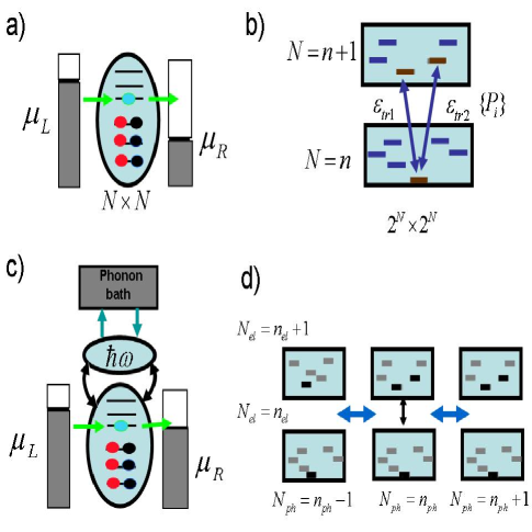
Figure 1: Introducing Fock Space transport. a) A schematic of electronic transport in the one-particle picture. The channel is coupled to two electrodes which add and remove electrons to and from the channel, resulting in current flow. Given a set of $N$ basis functions the transport problem computationally scales as $N\times N$. b) In the Fock space picture such addition and removal processes can be understood in terms of transitions between states that differ by a single electron number. In such a scheme one needs to keep track of all possible configurations in the channel, thus resulting in an exponential $2^{N}\times 2^{N}$ scaling of the transport problem. c) In case of strong electron-phonon interactions, the phonon system is coupled to a phonon bath which is maintained at equilibrium. d) The inclusion of phonons calls for using copies of the electronic Fock space, each corresponding to a phonon number. Electronic transport results in vertical transitions while phonon coupling results in horizontal ones.

In the following, we will progressively build complexity into our Fock space approach and attempt to identify the experimental ramifications of doing so.

II.1 A. Single level system, SCF analysis

Let us start with the smallest interacting system, namely, a real or artifical molecule with a single energy level capable of accomodating two spins (Fig. 2a). The onsite energy of the level is $\epsilon_{0}$ and the Coulomb charging energy $U$. The level is coupled to contacts which are held separately at thermal equilibrium at their respective bias-separated electrochemical potentials $\mu_{L,R}$ ($L$: left, $R$: right). A starting point for our analysis is the Hubbard Hamiltonian for the molecule

$$\hat{H}=\epsilon\hat{n}+U\hat{n}_{\uparrow}\hat{n}_{\downarrow}$$ (1)

where the operators $\hat{n}_{\uparrow,\downarrow}$ have eigenvalues 0 and 1, while $\hat{n}=\hat{n}_{\uparrow}+\hat{n}_{\downarrow}$. Exact diagonalizing this Hamiltonian leads to a Fock space consisting of four many-electron states (Figure 2(b)), an empty zero electron state $|00\rangle$ with energy $0$, two one electron states $|01\rangle$ and $|10\rangle$ corresponding to an up or a down spin with energy $\epsilon$, and a doubly occupied up-down spin electron state $|11\rangle$ with energy $2\epsilon_{0}+U$. Equilibrium occupancies of these many-electron states are given by the Boltzmann distribution $P_{N}=e^{-(E_{N}-\mu N)/k_{B}T}/\Omega$, where $k_{B}T$ is the thermal energy, $\mu=E_{F}$ is the equi librium contact Fermi energy or electrochemical potential, and $\Omega=\sum_{N}e^{-(E_{N}-\mu N)/k_{B}T}$ is the grand partition function. The average electron occupancy is then given by $\langle N\rangle=\sum_{N}NP_{N}$.

One can bypass the many-electron Fock space treatment by employing a suitable self-consistent (SCF) potential acting in the one-electron subspace, modifying the energies accordingly. In the spin restricted approach that treats both spins equally,

$$U_{RSCF}=\langle{\partial\hat{H}}/{\partial N}\rangle.$$ (2)

where $\langle\ldots\rangle$ denotes a quantum mechanical average. The interacting term can be written as

$$H_{int} = U\hat{n}_{\uparrow}\hat{n}_{\downarrow}$$

$$= U/2\sum_{\sigma}\hat{n}_{\sigma}\hat{n}_{\bar{\sigma}}$$

$$= (U/2)\sum_{\sigma}\hat{n}_{\sigma}(N-\hat{n}_{\sigma})$$

$$= (U/2)N\sum_{\sigma}\hat{n}_{\sigma}-(U/2)\sum_{\sigma}\hat{n}_{\sigma}^{2}$$

$$= UN(N-1)/2,$$ (3)

where we have used the fact that $N=\sum_{\sigma}\hat{n}_{\sigma}$, and $\hat{n}_{\sigma}^{2}=\hat{n}_{\sigma}$, since $\hat{n}$ can only take values of zero or one. The spin restricted SCF potential is then given by

$$U_{RSCF}=\langle\partial H_{int}/\partial N\rangle=U(\langle N\rangle-1/2)$$ (4)

For a given electrochemical potential, one guesses the value of the average occupancy $\langle N\rangle$, uses it to calculate the SCF potential, and then calculates in turn the mean-field occupancy $\langle N\rangle$ of the level $\tilde{\epsilon}=\epsilon+U_{SCF}$ using the Fermi-Dirac distribution $f(\tilde{\epsilon})=1/[1+e^{(\tilde{\epsilon}-\mu)/k_{B}T}]$, proceeding along this line until self-consistent convergence.

It is easy to see that the equilibrium occupancy $N-\mu$ rbhasko2 with respect to chemical potential (we drop the angular term indicating average here) should be qualitatively different between the SCF and many-body results. In the former, the electron occupancy is a fractional amount, adiabatically changing from zero to two. In the many-body result, however, one does not simply multiply the results for one electron by two, but the electron occupancy changes abruptly between zero to one, followed by a plateau of width $U$ over which the electrons are blockaded by the Coulomb interaction, after which the electron number reaches two abruptly.

One could capture this Blockaded effect using an unrestricted self-consistent potential (USCF) by dictating that the up and down spins do not feel potentials due to themselves. By eliminating this self-interacting, the unrestricted potential for a particular spin is then given by

$$U_{USCF} = \langle\partial H_{int}/\partial\hat{n}_{\sigma}\rangle$$ (5)

$$= Un_{\bar{\sigma}}$$

$$= U(N-n_{\sigma})$$

with $n=\langle\hat{n}\rangle$ and $\bar{\sigma}$ represents the spin opposite to $\sigma$. This spin-dependent unrestricted potential eliminates the self-interaction of the level to which charge is being added. A self-consistent solution of the occupancy yields an $N-\mu$ rbhasko2 plot very similar to the exact result, showing that an unrestricted calculation can capture equilibrium Coulomb Blockade effects.

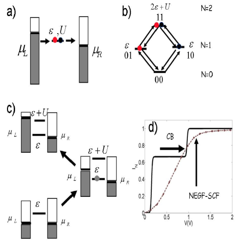
Figure 2: Fock Space transport through a singly degenerate energy level. a) The singly degenerate energy level can carry two electrons, one of each type. b) The Fock space thus comprises of $4$ states. Transitions between these result in c) two transport channels $\epsilon$ and $\epsilon+U$. Successive access of these transport channels results in two current jumps at different bias points separated by a plateau. A NEGF-SCF calculation is shown dotted for comparision.

II.2 B. Single level system, Fock space transport

Non-equilibrium turns out to be hard to mimic with any SCF theory, even with considerable latitude in our choice of the SCF potential. Let us assume the contact injection rates are given by $\gamma_{1,2}/\hbar$, ignoring level broadening for the moment. Here 1,2 also refers to the left (L) and right (R) contact. Both conventions are used in this paper to be consistent with NEGF literature. One can write down a master equation for a transition between the many-electron levels driven by the contacts

$$\dot{P_{i}}=-\sum_{j}R_{ij}P_{i}+\sum_{j}R_{ji}P_{j}$$ (6)

where $i,j$ represent the many-body states. The master equation, intuitively quite transparent from Figure 2(b), can be formally derived by decoupling the contact and molecular density matrix equations in the steady-state limit and then invoking a Markov approximation that ignores memory effects such as energy-dependences in the contact broadening. For our simple example of the dot with two spin levels, the transition rates between the four Fock states, numbered as $\{|00\rangle,|01\rangle,|10\rangle,|11\rangle\}$, are given by

$$R_{00\rightarrow 01} = R_{00\rightarrow 10}=(\gamma_{1}f_{1}+\gamma_{2}f_{2})/\hbar$$

$$R_{01\rightarrow 00} = R_{10\rightarrow 00}=(\gamma_{1}\bar{f}_{1}+\gamma_{2}\bar{f}_{2})/\hbar$$

$$R_{01\rightarrow 11} = R_{10\rightarrow 11}=(\gamma_{1}{f^{\prime}}_{1}+\gamma_{2}{f^{\prime}}_{2})/\hbar$$

$$R_{11\rightarrow 01} = R_{11\rightarrow 10}=(\gamma_{1}\bar{f^{\prime}}_{1}+\gamma_{2}\bar{f^{\prime}}_{2})/\hbar$$ (7)

where $f_{1,2}=1/[1+e^{(\epsilon_{0}-\mu_{1,2})/k_{B}T}]$, $\bar{f}_{1,2}=1-f_{1,2}$, $f^{\prime}_{1,2}=1/[1+e^{(\epsilon_{0}+U-\mu_{1,2})/k_{B}T}]$, and $\bar{f^{\prime}}_{1,2}=1-f^{\prime}_{1,2}$. In short, electron addition processes are governed by probability of occupancy $f$ at the corresponding transition energies $\epsilon$ or $\epsilon+U$ by each contact electrochemical potential, while electron removal processes are governed by the probability of vacancy $1-f$. Thus the two current onset points occur at the bias situations shown schematically in Figure 2(c).

At steady-state, it is straightforward to solve these equations (only three of which are independent), along with the normalization $\sum_{i}P_{i}=1$. The probabilities are then used to calculate the current injected by one contact (say the left one, “L’) as

$$I^{L}=\sum_{i}(\pm e/\hbar)[-\sum_{j}R^{L}_{ij}P_{i}+\sum_{j}R^{L}_{ji}P_{j}]$$ (8)

where the rates $R^{L}$ are obtained by only considering the individual left contact contributions to the corresponding rate, for example, $R^{L}_{00\rightarrow 10}=\gamma_{1}f_{1}/\hbar$. The $\pm$ signs correspond to addition/removal of electrons by the left contact. The resulting I-V characteristic is shown in Fig. 2(d).

In an SCF treatment, the current, shown dotted in Figure 2(d) is obtained by solving the rate equations in the one-electron subspace. The electron occupancy is given by $N=(\gamma_{1}f_{1}+\gamma_{2}f_{2})/(\gamma_{1}+\gamma_{2})$, where the Fermi functions are evaluated at the energy $\tilde{\epsilon}=\epsilon+U_{SCF}$. The SCF potential in turn depends on $N$ as described earlier, so the calculation is done self-consistently. The converged energy is then used to calculate the current as $I=(2e/\hbar)\gamma_{1}\gamma_{2}/(\gamma_{1}+\gamma_{2})[f_{1}-f_{2}]$.

The RSCF model that treats spins equally tends to give an adiabatically increasing current that reaches its maximum contact-dominated value $2e/\hbar\times\gamma_{1}\gamma_{2}/(\gamma_{1}+\gamma_{2})$ when the contact electrochemical potential fully crosses the level. It is important to note that charging alone can smear out this current, leading to a low conductance value spread out over a wide voltage range comparable to $U$. The RSCF potential $U(N-1/2)$ causes a continuous shift in levels with charge addition, which is accomplished in fractions. The unrestricted approach USCF gives an intervening Coulomb Blockade plateau of width $U$ that separates the first spin addition (or removal) event from the second. The intervening ‘open shell’ plateau is at half the maximum value for complete level filling, which is understandable because the two spins are treated on an equal footing chemically, and therefore carry equal current.

Compared with the SCF results above, the exact solution of the many-body rate equations reveals an interesting surprise that is actually quite illuminating. Of all many-electron configurations, the 1-electron states (and only those) are doubly degenerate, giving us a normalization condition that differs from a simpler version that ignores spins and simply multiplies all results by two. As a consequence of this sum-rule, which takes Pauli exclusion into account (preventing double up or down spin states, for example), the exact value of the open-shell current plateau depends on the Fermi functions as $\gamma_{1}\gamma_{2}/[\gamma_{1}(1+f_{1})+\gamma_{2}(1+f_{2})]$ in the large charging ($U\rightarrow\infty$) limit. For sharp levels at positive bias ($f_{1}=1$, $f_{2}=0$), this reaches $\gamma_{1}\gamma_{2}/[2\gamma_{1}+\gamma_{2}]$. For the strongly non- equilibrium situation corresponding to equal resistive couplings ($\gamma_{1}=\gamma_{2}$), the Coulomb plateau carries two-third of the maximum closed-shell current, in contrast with the USCF result that gives a factor of half. This implies an interesting history dependence, in that the first spin added to the empty level carries more current than the second! If we keep track of the entire many-electron configuration space, it is easy to see that this counter- intuitive result arises because there are two ways of adding the first spin and only one way of adding the second (the other channel eliminated by exclusion). This subtlety is completely washed away when we choose to work in a reduced $N\times N$ (or $2N\times 2N$ for unrestricted) subspace instead of the full $2^{2N}\times 2^{2N}$ configuration space.

The SCF potential $\langle\partial H/\partial n\rangle$ was calculated by writing the electron operators $\hat{n}=\langle\hat{n}\rangle+\delta\hat{n}$, expanding the Coulomb term $U\hat{n}_{\uparrow}\hat{n}_{\downarrow}$ and dropping the correlation terms $\delta\hat{n}_{\uparrow}\delta\hat{n}_{\downarrow}$ completely, i.e., the Hartree-Fock approximation. One could include parts of the correlation term phenomenologically, by dictating that $\hat{n}_{i}\hat{n}_{j}\approx(1-g_{ij})\langle n_{i}\rangle\langle n_{j}\rangle$, with $g_{ij}$ representing the exchange-correlation hole. This is in the spirit of Kohn-Sham theory, where the potential is calculated by various approximate means. However, the effect of $g$ is simply to renormalize the charging energy $U$ that it adjoins, influencing at best the width, but not the height of the current plateaus. Thus, even for the simplest quantum dot, unrestricted potentials in the one-electron subspace cannot capture the nonequilibrium properties correctly.

It is further illuminating when a comparison between the USCF and exact model is performed. Recall that in the USCF approach, we introduce the aspect of “self interaction correction” as described in Eq. 5. Here, the presence of an electron of a particular spin adds a coulomb cost to the other, but not on itself. Fig. 3(b) shows the discrepancy between the USCF and the many-body transport calculations for a dot with two spin levels, coupled equally to two contacts (driving it far from equilibrium). As is clear from the results, the discrepancy is in the onset voltages, widths and heights of the various plateaus. While the plateau widths could be adjusted to fit the exact results by renormalizing the charging energies parametrically to account for correlation effects, the heights are independent of these values, and depend only on universal factors arising from Pauli exclusion, and cannot be fixed in such a straightforward way, or by the usual DFT approach of progressively improving on correlations in the electronic structure. The issue is further underscored by the fact that in the strongly asymmetric limit ($\gamma_{1}=100\gamma_{2}$), where the system is essentially driven into equilibrium with the left contact, the agreement between USCF and many-body results is substantially improved. It is worth clarifying at this time though that in the multilevel generalization, this correspondence becomes a lot harder to establish even near equilibrium, since even the number of current plateaus generated by a $2^{N}\times 2^{N}$ Fock space approach differs substantially from its $2N\times 2N$ USCF counterpart (unless the broadening functions bear enough poles through their energy-dependences to precisely account for those missing conductance peaks).

The situation gets simpler if we have asymmetric contacts $\gamma_{1}\gg\gamma_{2}$, so that the system approaches equilibrium with the left contact. As Fig. 3 (d) shows, the USCF agrees with the many-body limit in this asymmetric coupling case, as both approaches are dealing with a near-equilibrium problem. For positive bias on the weaker contact, the stronger contact keeps the level filled (which it can do in two ways, adding an up or a down spin, assuming the level was empty to begin with). For opposite bias, the stronger contact empties this level, which can now be done in only one way (up OR down depending on what occupied the level). The competition between ‘shell tunneling’ and ‘shell filling’ makes the I-V strongly asymmetric, with the first plateau half the second for positive bias on the weaker contact, and merging with the second for opposite bias. This ratio of one to two, observed experimentally rralph2 , arises in a straightforward way from our analyses since the ratio of the first and second plateau currents is given for positive bias by $(\gamma_{1}+\gamma_{2})/(2\gamma_{1}+\gamma_{2})\approx 1/2$ for $\gamma_{1}\gg\gamma_{2}$, and by $(\gamma_{1}+\gamma_{2})/(\gamma_{1}+2\gamma_{2})\approx 1$ for negative bias. The asymmetry arises from the difference in the number of spin addition and removal channels for positive and negative bias, and leads to an asymmetry in the current levels.

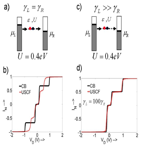
Figure 3: Comparison between USCF and exact transport results for (a) extreme non-equilibrium ($\gamma_{1}=\gamma_{2}$), b) in which the I-V’s show significant discrepancy between USCF (dotted red) and exact (bold black) result. c) The case of strong asymmetry implies a near equilibrium with the first contact ($\gamma_{1}=100\gamma_{2}$). d) The discrepancies in plateau onset, width and height are resolved in this equilibrium limit, but are hard to resolve once we go far from equilibrium.

We will next show how this model is extended for a larger molecule, and how additional physics due to correlations and excitations start to arise.

II.3 C. General Approach for multilevel systems

In case of a larger molecule, one begins with the model Hamiltonian in second quantized notation:

$$\hat{H} = \sum_{\alpha}\epsilon_{\alpha}\hat{n}_{\alpha}+\sum_{\alpha\neq\beta}t_{\alpha\beta}c_{\alpha}^{\dagger}{c_{\beta}}$$ (9)

$$+ \sum_{\alpha,\sigma}U_{\alpha\alpha}\hat{n}_{\alpha\sigma}\hat{n}_{\alpha\bar{\sigma}}+\frac{1}{2}\sum_{\alpha\neq\beta}U_{\alpha\beta}\hat{n}_{\alpha}\hat{n}_{\beta},$$

where $\hat{n}_{\alpha}=c^{\dagger}_{\alpha}c_{\alpha}$, $\alpha,\beta$ correspond to the orbital indices of the orbitals for various sites on the molecule, and $\sigma$,$\bar{\sigma}$ represent a particular spin and its reverse. Exact diagonalizing this Hamiltonian yields a large spectrum of closely spaced excitations in every charged molecular configuration. Using the equation of motion of the density matrix of the composite molecule and leads and assuming no molecule-lead correlations, one can derive timm ; rbraig a simple master equation for the density-matrix of the system. Ignoring off-diagonal coherences, we are left with a master equation rbraig in terms of the occupation probabilities $P^{N}_{i}$ of each N electron many-body state $|N,i\rangle$ with total energy $E^{N}_{i}$. The master equation then involves transition rates $R_{(N,i)\rightarrow(N\pm 1,j)}$ between states differing by a single electron, leading to a set of independent equations defined by the size of the Fock space rralph

$$\frac{dP^{N}_{i}}{dt}=-\sum_{N,j}\left[R_{(N,i)\rightarrow(N\pm 1,j)}P^{N}_{i}-R_{(N\pm 1,j)\rightarrow(N,i)}P^{N\pm 1}_{j}\right]$$ (10)

along with the normalization equation $\sum_{i,N}P^{N}_{i}=1$. For weakly coupled dispersionless contacts, parameterized using bare-electron tunneling rates $\gamma_{\alpha}$, ($\alpha$: left/right contact), we define rate constants

$$\Gamma_{ij\alpha}^{Nr} = \gamma_{\alpha}|\langle N,i|c^{\dagger}_{\alpha}|N-1,j\rangle|^{2}$$

$$\Gamma_{ij\alpha}^{Na} = \gamma_{\alpha}|\langle N,i|c_{\alpha}|N+1,j\rangle|^{2},$$ (11)

$c^{\dagger}_{\alpha},c_{\alpha}$ are the creation/annihilation operators for an electron on the molecular end atom coupled with the corresponding electrode. The transition rates are given by

$$R_{(N,i)\rightarrow(N-1,j)} = \sum_{\alpha=L,R}\Gamma_{ij\alpha}^{Nr}\left[1-f(\epsilon^{Nr}_{ij}-\mu_{\alpha})\right]$$

$$R_{(N-1,j)\rightarrow(N,i)} = \sum_{\alpha=L,R}\Gamma_{ij\alpha}^{Nr}f(\epsilon^{Nr}_{ij}-\mu_{\alpha}).$$ (12)

for the removal levels $(N,i\rightarrow N-1,j)$, and replacing $(r\rightarrow a,f\rightarrow 1-f)$ for the addition levels $(N,i\rightarrow N+1,j)$. $\mu_{\alpha}$ are the contact electrochemical potentials, $f$ is the corresponding Fermi function, with single particle removal and addition transport channels $\epsilon^{Nr}_{ij}=E^{N}_{i}-E^{N-1}_{j}$, and $\epsilon^{Na}_{ij}=E^{N+1}_{j}-E^{N}_{i}$. Finally, the steady-state solution to Eq.(10) is used to get the left terminal current

$$I=\pm\frac{e}{\hbar}\sum_{N,i,j}\left[R^{L}_{(N,i)\rightarrow(N\pm 1,j)}P^{N}_{i}-R^{L}_{(N\pm 1,j)\rightarrow(N,i)}P^{N\pm 1}_{j}\right]$$ (13)

where states corresponding to a removal of electrons by the left electrode involve a negative sign. We will assume a break-junction configuration with equal electrostatic coupling with the leads, $\mu_{L,R}=E_{F}\mp eV_{d}/2$.

While the above equations include spectral details from the multiple excitations, a considerable simplification arises if we can incoherently sum over many of these excitations, leading to the ‘orthodox model’, where

$$I=\pm\frac{e}{\hbar}\sum_{N}\left[R^{L}_{N\rightarrow N\pm 1}-R^{L}_{N\rightarrow N\mp 1}\right]P^{N}$$ (14)

The transition energies can be obtained in terms of a simple RC circuit, while the transition rates also compactify once we integrate them over the relevant energies, taking exclusion factors into account.

The implementation of the above sets of equations now sets the stage for further discussions.

III III. Coulomb Blockade: the case of electronic transport channels

In this section we describe how the excitation spectra of molecules may be probed using Coulomb Blockade transport. While typical molecular I-Vs look relatively featureless, what is not often appreciated is that in the Coulomb Blockade limit (realized by engineering weak contacts or non-conductive backbones), electronic excitations do give rise to prominent features in the I-V jpark ; zhitenev . We will also show how such an excitation spectra can generate intrinsic I-V asymmetries, which in turn can manifest itself as NDR effects.

Exact-diagonalization of the molecular Hamiltonian Eq. 9 generates a body of excitation spectra for every charged configuration. Our typical starting point is the equilibrium molecular quantum dot configuration in its ground state. Addition or removal of an electron takes the system to the a new ground state corresponding to the singly charged cation or anion, marking the onset of conduction. In addition to the ground state however, each charged species bears a quasi continuous excitation spectrum separated from its ground-state energy by a gap that is determined by the energetics of the molecular system. Once the first excitation is accessed, the quasi-continous excitation spectrum can be easily probed, as shown in Figures 4(a), (b) and (c). It is worth emphasizing that the excitations are energetically quite close as they differ in the rearrangement (but not in the number) of charges. At high bias with small broadening and in the absence of phonons, the purely electronic excitations do not have adequate time to relax to the ground state, accounting for their visibility in the current spectrum.

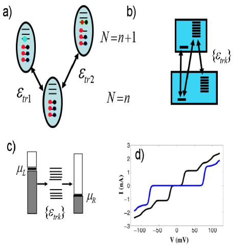
Figure 4: Electronic excitations in molecular conduction. a) Schematic shows three Fock states, the $N=n$ equilibrium ground state configuration and two states in the addition $N=n+1$ spectrum. b) Each charge configuration consists of a ground state and a set of closely spaced excitations. The access of such closely spaced excitations between the neutral and charged species gives rise to numerous c) transport channels $\epsilon_{trk}$ rbhasko1 . The access of such transport channels gives rise to a quasi ohmic behavior in the I-V characteristics that are commonly noted in various experiments rweber1 ; rweber2 .

The simplest and most prominent impact of Coulomb Blockade on the I-Vs of short molecular wires is a clear suppression of zero-bias conductance, often seen experimentally rreed ; rtao . However, integer charge transfer can also occur between various electronic excitations of the neutral and singly charged species at marginal correlation costs rfulde ; gus . The above fact leads to fine structure in the plateau regions jpark ; rweber1 ; rweber2 ; pnas , specifically, a quasilinear regime resulting from very closely spaced transport channels ($\epsilon^{N}_{ij}$) via excitations. The crucial step is the access of the first excited state via channel $\epsilon^{Nr}_{10}$, following which transport channels involving higher excitations are accessible in a very small bias window.

The sequence of access of transport channels upon bias, enumerated in the state transition diagrams shown in Figs. 4(a),(b) and (c) determines the shape of the I-V characteristic. When the Fermi energy $E_{F}$ lies closer to the threshold transport channel $\epsilon^{Nr}_{00}$ corresponding to charge transfer between two ground states, it takes an additional positive drain bias for the source to access the first excited state of the neutral system via the transition $\epsilon^{Nr}_{10}$. Under this condition, the I-V shows a sharp rise followed by a plateau (Figure 4(d), shown in blue), as seen in various experiments rdekker . However, when transport channels that involve low lying excitations such as $\epsilon^{Nr}_{10}$ are closer to the Fermi energy $E_{F}$ than $\epsilon^{Nr}_{00}$, the excitations get populated by the left contact immediately when the right contact intersects the threshold channel $\epsilon^{Nr}_{00}$, allowing for a simultaneous population of both the ground and first excited states via $\epsilon^{Nr}_{00}$ and $\epsilon^{Nr}_{10}$ at threshold. Under these conditions the I-V shows a sharp onset followed immediately by a quasilinear regime (Fig. 4(d) shown in black) with no intervening plateaus, as observed frequently in I-Vs of molecules weakly coupled with a backbone rweber1 ; rweber2 ; jpark .

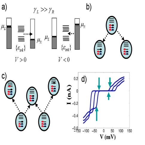
Figure 5: Current asymmetry from extrinsic “contact” asymmetry. a) In the case when the left electrode is more strongly coupled to the channel than the right one $\gamma_{L}>>\gamma_{R}$, currents are limited by removal (addition) rates under forward (reverse) bias conditions. b) The number of removal channels can be significantly different from the number of c) addition channels. This gives rise to the asymmetry between d) forward and reverse bias situations. Furthermore the application of gate potential modulates the number of transport channels available at threshold. This feature results from the Fock space excitation spectra, causing not only a change in threshold voltage with applied gate bias, but also a discernable threshold current modulation as noted here, and in various experiments jpark .

III.1 A. Extrinsic Asymmmetries -the case of rectification

The direct role of excitations in conduction becomes particularly striking under asymmetric coupling ($\gamma_{L}>>\gamma_{R}$) with contacts jpark ; rscott . Due to this extrinsic asymmetry, current magnitudes are dictated by the weaker contact. This asymmetry directly affects the forward and reverse bias characterestics, leading to current rectification. This rectification is caused by the inherent asymmetry between addition and removal processes, each of which is the rate limiting depending on the bias direction, as shown in Figs. 5(a), (b) and (c).

In contrast to the SCF regime where unequal charging drags out a same level current over different voltage widths rasymm , in the CB regime we encounter clear intermediate current steps from open shells, with current heights that are themselves are asymmetric at threshold (Fig. 5(d)). This asymmetry arises due to the difference in the number of pathways for removing or adding a spin, taking in particular into account the possible excitation channels between the neutral and singly charged species (Figures 5(b) and (c)). The number of such accessible excitations at threshold can be altered with an external gate bias, leading to a prominent gate modulation of the threshold current heights, over and above the modulation of the onset voltages and the conductance gap jpark (Figure 5(d)). Furthermore, it is easy to show that the asymmetry will flip between gate voltages on either side of the charge degeneracy point, as is also observed experimentally rscott .

It is worth emphasizing that the sophistication arose specifically due to the presence of separate identifiable contributions from the open shells, which are normally overwhelmed by broadening if we were away from the CB limit. However, the specific identification of these excitations is not crucial to the qualitative shape of the I-Vs, as long as one is not looking too closely at the individual spectral features. A simpler orthodox model would then suffice to reproduce these broad features described above, such as the transition between steps and slopes in the I-Vs, the flipping of asymmetry and the gate modulation of the current levels rowen . However, there are notable exceptions, such as intrinsic asymmetries, where a clear separation needs to be made between certain classes of excitations with longer lifetimes (‘traps’) and the regular excitations with shorter lifetimes (‘channels’) that are responsible for the current flow.

III.2 B. Intrinsic Asymmetries - NDR, hysteresis and telegraph noise

The physics of NDR can be explained readily using an USCF model that is actually quite intuitive. Consider a channel and a trap, the channel being strongly coupled to the contacts and the trap weakly coupled. Accessing the channel creates a resonant onset of current. Accessing the trap subsequently would keep the conduction unaffected, as the trap is non-conducting; however, once we throw in the strong Coulomb repulsion arising from charging up the trap, it is easy to see that this repulsion can expel the conducting channel out of the conducting bias window, leading to an NDR. Self-interaction correction is crucial to this picture, as the charging should repel the channel level, but not the trap level itself. Further sophistications can arise by considering the lifetime of the trap. If the trap does not release its charge during the measurement time, then a reverse scan would keep the channel blocked and lead to a hysteresis. Such a hysteresis is scan-rate dependent, as the rate determines the degree to which the trap releases its captive charge. The low current state can be reversed by going to large negative bias to expel this charge and restore initial conditions.

The realization of the NDR involves two conditions: (a) that the charging of the trap is large enough to expel much of the channel from the bias window, and (b) that the resulting current carried by the trap plus the residual tail of the channel sitting in the bias window exceeds the current carried originally by the channel alone. The first amounts to the onset condition for an NDR, while the second describes, in some sense, the effectiveness of the NDR (in terms of an inequality). With a little bit of effort, one can extract a range of parameters that satisfy both these conditions. We will instead show that even in the Fock space picture (which treats the channel plus trap as a composite system), one can identify these two same conditions: the NDR starts when one encounters what we refer to as a ‘dark’ or ‘blocked’ state, and subject to this condition, the effectiveness of the NDR amounts to an inequality that we will now discuss.

A condition for NDR can be derived much more generally in terms of three Fock space states $|A\rangle$, $|B\rangle$, and $|C\rangle$ with energies $E_{A}<E_{B}<E_{C}$ respectively (Fig 6(a)), representing three accessible states within the bias range of interest. For instance, $|A\rangle$, $|B\rangle$ could be the ground states of the $N=n_{0}$ and $N=n_{0}+1$ electron systems, while $|C\rangle$, the first excited state of the $N=n_{0}+1$ electron system. Transport of electrons involves single charge removal or addition between states $|B\rangle$, $|C\rangle$ and $|A\rangle$ that differ by an electron, via addition and removal rates $R_{A\leftrightarrow B,C}\propto\frac{1}{\tau_{AB,C}}$. Such an electron exchange is initiated when reservoir levels are in resonance with the single electron transport channels $\epsilon_{BA}=E_{B}-E_{A}$ and $\epsilon_{CA}=E_{C}-E_{A}$ respectively. The I-V characteristic of this three state system, shown schematically in Fig 6(b), shows two plateaus with current magnitudes $I_{a}$ and $I_{b}$ respectively. Current collapse or NDR occurs when $I_{a}>I_{b}$.

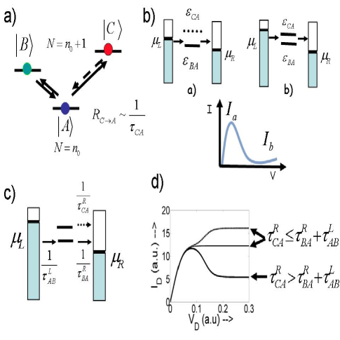
Figure 6: NDR effects from intrinsic asymmetry or “dark states”. a) A generic mechanism NDR can be cast in terms of three device Fock-space states, and transitions $\mid A\rangle\leftrightarrow\mid B\rangle$ and $\mid A\rangle\leftrightarrow\mid C\rangle$ between those that differ by a single electron. The dark state $\mid C\rangle$ say has a very slow removal rate in comparison to its addition rate. b) Bias environments, a and b, correspond to current rise followed by a collapse. c) A general criteria for such a current collapse or NDR to occur with increasing voltage can be cast in terms of the dark state removal rates. d) NDR in the I-V characteristic is contingent to the criteria derived here rbhasko3 .

In the above system, NDR occurs when under specific conditions, the state $|C\rangle$ can be a blocking or dark state, for which electron addition is feasible while removal is rate limiting. This can happen when there are intrinsic asymmetries within the transport problem, as in the trap-channel dichotomy described earlier. Regardless of the specific origin of blocking, a simple criteria for current collapse can be derived rbhasko3 in terms of the rate limiting process, that is the electron removal rate $R_{C\leftrightarrow A}$ from the dark state $|C\rangle$. A better intuition is provided by thinking of rates as inverse lifetimes, as shown in Figure 6(c). If the life time of state $|C\rangle$, $\tau_{CA}$ exceeds the sum of the addition and removal rates of the conducting state, it becomes an effective blocker. In other words, the condition $\tau^{R}_{CA}>\tau^{L}_{AB}+\tau^{R}_{BA}$ determines whether NDR occurs or not. The superscripts $L$ and $R$ represent left or right electrode, and under the forward bias situation add and remove electrons respectively. The consequence of the above criterion is summarized in Figure 6(d), clearly indicating that NDR only occurs when $\tau^{R}_{CA}>\tau^{L}_{AB}+\tau^{R}_{BA}$. A similar criteria is valid for the reverse bias direction by interchanging superscripts $L$ with $R$.

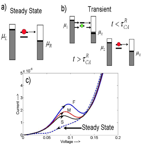
Figure 7: Hysteresis effects due to sweep rate. a) Under steady state conditions the dark state behaves as an effective blocker. b) A sweep rate faster than the rate determining time scale can put the transport process in a transient state. c) Under such transient conditions sweep rate can induce disguised NDRs and often hysteresis, both depending on sweep rate kiehl .

Further sophistications may arise due to ‘transient’ probing. The criteria obtained above applies for steady state, where the dark state gets occupied with certainty, resulting in an inevitable current blockade regimee. Let us consider such a blocked current state, shown dotted in Figure 7(c). A ‘disguised’ NDR can also be achieved if the voltage sweep rates are faster than the rate determining dark state life time. Such a sweep rate simply means that the dark state has not yet been occupied and thus a current determined by the addition and removal times ${1}/({\tau^{L}_{AB}+\tau^{R}_{BA}})$, can still flow. This situation is shown in Figure 7(c), in which the onset of dark state can be delayed provided the sweep rate is fast enough. But once the dark state forms, the current is blocked and thus remains so. This implies that on the backward sweep current remains blocked, resulting in a sweep rate-dependent hysteresis. Such a behavior has been noted by Kiehl et.al. kiehl in a molecular system, which was attributed to a slow charge trapping process, which again fits into the dark state picture. Just as noted here, Kiehl et.al. also observe that the NDR effect diminishes with decreasing sweep rate and ultimately vanishes at steady state, implying the absence of a real hysteresis at steady state. This kind of hysteresis is just an artifact of sweep rates being faster than the rate determining processes.

It must be mentioned that certain hysteretic processes can occur even at steady state due to the true bistable nature of the system. A classic example is the charging induced hysteresis in resonant tunneling diode (RTD) structures cap . Other interesting examples include bistability caused by hyperfine interactions tar2 causing a hysteresis with applied magnetic field, and optical bistability created by superlattice dielectrics that show strong terahertz nonlinearity due to Bloch oscillation and dynamic localization of electrons thz1 ; thz2 .

While we discussed the interesting case of dark states earlier, touching upon relevant consequences such as NDR and hysteresis, we avoided particular examples. Recently, we applied our dark state model rbhasko3 to explain the NDR observed due to subtle spin correlation effects in double quantum dots tar . Indeed this NDR results in the spin blockade regime tar which currently forms a key concept in the area of single spin manipulation and control kow ; pet ; cm ; kw ; now .

Finally, the transient probing with a high resolution probe would allow us to explore the approach to resonance with the trap states. As we discuss in ghoshieee , the stochastic blocking and unblocking of the channel by the occupation/deoccupation of the traps near resonance generates a flicker in the output current known as random telegraph noise. The ratio of capture and emission times is given by a Boltzmann factor whose argument depends on the trap energy location. Shifting this trap with a combination of gate and drain voltages leads to an associated scaling of the capture to emission time ratio, allowing one to infer the spatial and spectral location of the trap states. This provides a powerful ‘barcode’ for characterizing single-molecular defects.

Our analyses over the last few sections focused on electron-electron correlations and their treatment in a Fock space approach that captures the relevant physics (if at the expense of computational simplicity). In the next section, we will discuss how this approach can be extended to incorporate electron-phonon correlations in transport.

IV IV. Electron-phonon Interactions:

So far, our primary concern was Coulomb Blockade and electronic excitations. Here, we show that coupling Coulomb Blockade with phonon-assisted tunneling results in non-trivial physics. This section is primarily motivated by a recent series of experiments performed on suspended carbon nanotube quantum dots leroy . In such a suspended system, the phonons are driven far out of equilibrium and couple strongly with the electronic system. Our approach then is to invoke the Fock space of the electron phonon system as indicated in Figures 1(c) and (d).

IV.1 A. SCF treatment – IETS and phonon sidebands

The SCF approach to electron-electron interactions has been discussed at length in our earlier papers and contrasted with the Fock space approach. It is worth quickly touching upon the SCF treatment of phonons, before diving into its Fock-space analogue. In presence of dephasing scattering events, the current at the left contact can be written in the NEGF formalism rdatta1 as

$$I_{L}={{2e}\over{h}}\int dETr[\Sigma_{L}^{in}A-\Gamma_{L}G^{n}]$$ (15)

where $A$ is the spectral function, $\Gamma_{L}$ is the broadening by the left contact, $\Sigma_{L}^{in}$ is the in-scattering self-energy from the left contact and $G^{n}$ is the correlation function describing the energy-dependent occupancy of the levels, taking quantum interference into account. The influence of scattering by contacts and phonons sits in $\Sigma^{in}=\Sigma^{in}_{L}+\Sigma^{in}_{R}+\Sigma^{in}_{ph}$. The equations for the contact $\Sigma$s are well known – we will focus here on the additional contributions from the phonon scattering processes. Within the self-consistent Born approximation (self-consistency needed to conserve current), the equations connecting the phonon contributions form two groups – a set of dynamic equations, and a set of static equations. The non-equilibrium dynamics describing the filling and emptying of states is described by

$$G^{n,p}(E) = G(E)\Sigma^{in,out}_{ph}(E)G^{\dagger}(E)$$

$$\Sigma^{in,out}_{ph}(E) = D_{0}(\omega)\otimes\Biggl{[}n_{B}(\omega)G^{n,p}(E\mp\hbar\omega)\Biggr{.}$$

. $$+ \left(n_{B}(\omega)+1\right)G^{n,p}(E\pm\hbar\omega)\Biggr{]}$$ (16)

where $n_{B}(\omega)=[e^{\hbar\omega/k_{B}T}-1]^{-1}$ is the equilibrium Bose-Einstein distribution of the phonons, and $D_{0}$ is its deformation potential, in other words, $(D_{0})_{ij}=h_{i}h_{j}$, $h_{\alpha}$ being the electron phonon coupling constant at the real space point $\alpha$ (In general, $h$ is a non-diagonal matrix in an arbitrary basis set, and $D_{0}$ is a fourth-rank tensor). $\otimes$ denotes an element-by-element (as opposed to matrix) multiplication. The equations above are for a single phonon mode at frequency $\omega$, and will need to be integrated over a phonon density of states for a continuous distribution of phonons.

The static equations describing the states themselves are given by

$$\Gamma_{ph}(E) = \Sigma^{in}_{ph}(E)+\Sigma^{out}_{ph}(E)$$

$$\Sigma_{ph}(E) = {\cal{H}}(\Sigma_{ph})+i\frac{\Gamma_{ph}}{2}$$

$$G(E) = [EI-H-\Sigma_{L}-\Sigma_{R}-\Sigma_{ph}]^{-1},$$ (17)

where ${\cal{H}}$ denotes the Hilbert transform. The above equations capture the physics of phonon-assisted tunneling in all its various limits. In its simplest form, it contributes to dephasing that reduces the ballistic current in devices. Near resonance, the $\pm\hbar\omega$ terms in the arguments of the $G^{n,p}$ matrices contributing to $\Sigma^{in,out}(E)$ generate phonon sidebands. The scaling of these sidebands depends on the deformation potential as well as the distribution of the phonons. We have assumed this to be equilibrium Bose-Einstein $n_{B}$, although one could generalize it provided we have a separate evolution equation for the phonon dynamics coupled to the electron transport equations that describe parametrically or otherwise how the phonons are driven away from equilibrium by the electronic subsystem, and how the other terms in the phonon evolution equation (typically involving coupling with a thermal reservoir) try to bring this back to equilibrium. In the next section, we will, in fact, include these ‘hot’ phonon equations explicitly; instead of separate coupled equations, however, we will treat the electron-phonon as a composite system, and use the couplings between the electrons, phonons, and with the contacts and the bath as processes driving the evolution of the composite system.

The NEGF formalism also allows us to get away from this phonon-assisted tunneling limit to the off-resonant limit. When the electronic levels lie far from resonance, their sidebands do not show up and we get instead the inelastic electronic tunneling spectrum (IETS) of the molecular system. For weak electron-phonon coupling (retaining leading order terms in $D_{0}$), the NEGF algebra simplifies considerably, so that the current partitions into an elastic component given by the usual Landauer formula, as well as an inelastic component that explicitly involves exclusion principle terms at different emission and absorption energies. For applied voltages larger than the phonon frequency, these terms create additional current transport channels through phonon emission, creating a slight increase in the current that only shows up as peaks in the second derivative with voltage, generating the familiar IETS spectrum. The physics resides entirely in the inelastic current – one can use sophisticated electron structure methods to extract these peak positions from the phonon frequencies, as well as the IETS peak heights from the computed deformation potentials. The results also show additional subtleties near resonance that are experimentally observed. Specifically, near resonance the elastic current also picks up phonon signatures from the phonon contributions to $\Sigma$ residing in $G$, generating a dip rather than a peak that arises from the phonon sidebands described above (the equations also generate a familiar polaronic shift of the main peak). The inclusion of the equilibrium $n_{B}$ distribution gives phonon emission peaks that are stronger in strength than absorption peak by Boltzmann ratios evaluated at the electronic temperature.

While encouraging agreement between computed and experimental off-resonant behavior, specifically, IETS spectra has been reported rpaulsson , the resonant phonon sidebands and the scaling of their conductance peak heights with current shows significantly more complex behavior arising from strong non-equilibrium electron-phonon correlations, which necessitates a Fock space approach. We will now introduce the joint electron-phonon Fock space and the experimental ramifications of electron-phonon correlation effects captured with this treatment.

IV.2 B. Fock space treatment of phonon sidebands

We start from a model Hamiltonian for a quantum dot having onsite energies $\epsilon_{i}$, Coulomb interaction energy $U_{ii^{\prime}}$, vibronic modes at energy $\hbar\omega_{j}$ and electron-phonon coupling $\lambda_{ij}$. The system is connected to electrical contacts with couplings $\Gamma_{1,2}$ and to a thermal bath with coupling $\beta$ (figure 8(a)). Electronic transport due to bias applied to the contacts as well as phonon emission and absorption processes lead to transitions between many-body states $|e_{Ne}^{i},k\rangle$ ($k$ phonons and ith electronic level in the $N_{e}$ electronic subspace) of the quantum dot (figure 8(b)). The rates of these transitions due to left (right) contact ($\mathcal{R}^{L(R)}_{|e_{Ne-1}^{r},k\rangle\to|e_{Ne}^{s},p\rangle}$) and the phonon bath ($\mathcal{R}^{ph}_{|e_{Ne-1}^{r},k\rangle\to|e_{Ne}^{s},p\rangle}$) are calculated by applying Fermi’s Golden Rule lutfe . When an electron is added or removed via standard transport processes, it can also change the number of phonons, taking the dot from a state $|0,N\rangle$ to $|1,N\pm p\rangle$ or vice versa, where $p$ is the number of phonons emitted or absorbed. When the quantum dot absorbs or emits a phonon, the state changes from $|X,N\rangle$ to $|X,N\pm 1\rangle$, where $X=0$ or $1$. The consequence of phonons in transport is the addition of extra transport channels to the already existing Coulomb Blockade transport channels, as shown in Figures 8(c) and (d).

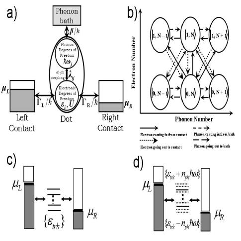
Figure 8: Fock space model to include electron-phonon interactions. a) The dot is electrically connected to the left (right) contact (with electron tunneling rates $\Gamma_{L,R}/\hbar$) and mechanically to the phonon bath (with a phonon escape rate of $\beta/\hbar$). The dot has electronic degrees of freedom $\epsilon_{i}$ and phonon degrees of freedom $\hbar\omega_{j}$ ($i,j=1,2,3,\ldots$) with coupling $\lambda_{ij}$. b) Transition between different states of a dot, having one electronic level and one phonon mode, due to coupling to the contact and the phonon bath ($|0,N>$ and $|1,N>$ denotes the states of the system having $N$ phonons each but $0$ electron and $1$ electron respectively). c) Effective Coulomb blockaded channel in the absence of phonons. d) Inclusion of electron-phonon coupling adds phonon side bands to the existing transport channels.

The rate equations in the above Fock space (8) can be solved for a finite number of phonon emission or absorption channels to extract the resulting current-voltage characteristic. Focusing on the intriguing experiments on Coulomb Blockaded nanotube quantum dots with prominent breathing modes leroy , one sees multiple intriguing features: (a) the absorption and emission sideband heights do not scale as simply as above. This is because the number of phonons $N_{ph}$ itself changes with current, in addition to being driven far from equilibrium in the suspended sections of the tube with small escape rate $\beta$. (b) The scaling of sidebands with phonon population differs significantly from predictions of the analogous Tien-Gordon theory of photon-assisted tunneling (PAT) rtg . This discrepancy arises because unlike the PAT experiments, the phonons are not coherent, and are partly correlated with the nanotube electrons lutfe

IV.3 C. Non-equilibrium phonons and effective temperature

A crucial component of the above picture is the strongly non-equilibrium distribution for the phonon population, as their generation rate by the drive current (determined by $\Gamma_{L,R}$ and $\lambda$) exceeds their extraction rate $\beta$. From the solution to the rate equations giving us the joint electron-phonon occupation probabilities, we can calculate the probability distribution of the phonon by summing over the electronic subspaces: $P^{ph}_{k}=\sum_{s,Ne}P_{|e^{s}_{Ne},k\rangle}$. Defining an effective temperature $T^{*}$ corresponding to the non-equilibrium phonon occupation $N_{ph}=[e^{\hbar\omega/k_{B}T^{*}}-1]^{-1}$, we find the corresponding Boltzmann distribution: $P^{phB}_{k}=e^{-k\hbar\omega/k_{B}T^{*}}/Z$ of phonon subspace occupation probability, where $Z$ is the partition function ($T^{*}$ is identified by fitting the higher energy tails between the two distributions). A comparison between $P^{ph}_{k}$ and $P^{phB}_{k}$ at different bias for different decay rates of the phonons reveals that they differ considerably as the phonon decay rate $\beta/\hbar$ decreases (figure 9(a)) at some applied bias. The deviation from a Bose-Einstein like shape suggests that the phonons in the suspended nanotubes are strongly non-equilibrium, so that temperature is not a well-defined quantity except to describe the higher energy tails (figure 9(b)).

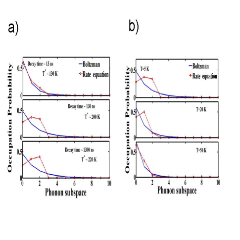
Figure 9: The phonon distribution $P^{phB}_{k}$ from the Boltzmann dist. a)(solid line) with the effective temperature $T^{*}$ differs considerably from the phonon distribution $P^{ph}_{k}$ calculated directly from the rate equation (circles). b) The phonon distribution $P^{ph}_{k}$ approaches the Boltzmann distribution $P^{phB}_{k}$ (with proper effective temperature $T^{*}$ not shown here) at elevated surrounding temperature $T$.

IV.4 D. Effect of the surrounding temperature: anomalous phonon population

The non-equilibrium phonon population reveals a striking and somewhat counter-intuitive dependence on the substrate temperature, the phonon population decreasing with increasing temperature at certain bias voltages (Fig. 10(a)). This peculiar behaviour manifests itself as long as the surrounding temperature is smaller than the separation between the upper emission and lower absorption sidebands of two subsequent Coulomb Blockade peaks. Beyond this temperature the phonon occupancy increases monotonically with temperature for all bias values, as expected. The anomalous temperature dependence arises from a trade-off between phonon generation and recombination rates in the coupled dot-lead-bath system. The behavior is observed specifically at bias values corresponding to the onset of a new phonon absorption channel (Figure. 10(b), bottom left). With increasing temperature from $\sim$ 5 to 20K, the increasing tails of the contact Fermi functions redistribute the electrons from a phonon emission sideband $\epsilon_{1}+\hbar\omega$ of a lower electronic peak to an absorption sideband $\epsilon_{2}-\hbar\omega$ of a higher peak (Figure. 10(b) bottom right). Under this specific conspiracy of temperature and bias values, the number of electrons resonant with the phonon sidebands decrease with increasing temperature, decreasing the efficiency of the phonon-assisted transport. At higher temperatures between 20-50 K, the temperature is large enough to open new emission channels that eventually increases the phonon population at all bias voltages.

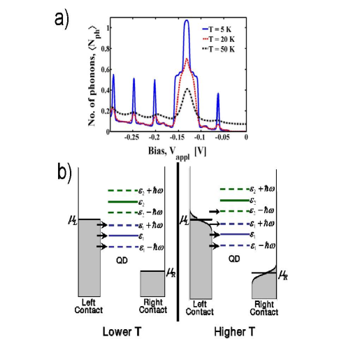
Figure 10: Anamolous temperature dependence of phonon distribution a) The number of phonons decreases at some bias points with increasing surrounding temperature $T$. (b) Bottom LeftAt lower surrounding temperature excitation of energy $\epsilon_{1}+\hbar\omega$ associated with resonant level $\epsilon_{1}$ falls inside the bias window between $\mu_{L}+k_{B}T_{L}$ and $\mu_{R}-k_{B}T_{R}$ and the excitation of energy $\epsilon_{2}-\hbar\omega$ associated with resonant level $\epsilon_{2}$ falls outside the bias window. Bottom right: At elevated surrounding temperature fermi functions of the contacts broadens around respective chemical potentials and the excitation of energy $\epsilon_{2}-\hbar\omega$ enters the bias window and lesser no. of electrons appear at energy $\epsilon_{1}+\hbar\omega$ in the left contact.

V Concluding Remarks

For a wide variety of transport problems, a perturbative treatment of interactions coupled with a quantum kinetic theory (such as NEGF) does an admirable job of explaining and predicting experimental features and providing important physical insights. As objects scale towards nanodimensions, however, strong confinement and poor coupling with the surroundings lead to increasing degrees of correlation, especially at lower temperatures. In this limit, the Fock space approach (more generally, the many-body density matrix approach) naturally allows us to compute transport signatures, provided we have a suitable means of extracting the various correlated many-body states and the transition rates among them. Exact diagonalization provides one option, although this quickly becomes computationally intractable. Partial configuration interaction (CI) schemes may prove to be more practical. In contrast with the NEGF-SCF limit where one could aim for quantitative and predictive accuracy with increasing amounts of chemical sophistication, such details are hard to build into the Fock space approach and need to be replaced by simpler, model problems, with parameters that could be benchmarked with more detailed models and measurements. However, even these simple models (with a reasonable choice of parameters) show qualitatively new physics that is experimentally observable, ranging from gate-modulated current levels, gate tunable excitation spectra, scan-rate dependent NDR and hysteresis, and the breakdown of our common intuition based on equilibrium phonon sideband scaling and the classical theories of photon-assisted tunneling. While these two limits (quantum wire and quantum dot) are separately well understood, at least formally, the intermediate coupling regime between the two becomes particularly challenging to model as there is no small ‘fine structure’ parameter that would allow a convenient starting point for a perturbation expansion (e.g. a noninteracting wire or a fully interacting but isolated quantum dot). Significant progress is needed at formal, computational and experimental levels in order to probe this regime, which bears the promise of completely novel physics of non-equilibrium correlations as well as possible applications based on the interaction between conducting detector elements in the quantum wire regime and non-conducting storage elements in the quantum dot regime.

Acknowledgements: It is our pleasure to acknowledge Prof. Supriyo Datta for useful discussions.

References

References

- (1) M. Lundstrom, and J. Guo, Nanoscale Transistors:Device Physics, Modeling and Simulation, Springer, New York, (2005).
- (2) M.A. Reed., C. Zhou, D.J. Muller, T.P. Burgin, and J.M. Tour, Science 278, 252 (1997).
- (3) J. Chen, M. A. Reed, A. M. Rawlett. J. M. Tour, Science, 286, 1550 (1999).
- (4) W.G. van der Weil, S. DeFranceschi, J. M. Elzerman, T. Fujisawa, S. Tarucha, and L. P. Kouwenhoven, Rev. Mod. Phys. 75, 1 (2003) and references therein.
- (5) R. Hanson, L. P. Kouwenhouven, J. R. Petta, S. Tarucha, and L. M. K. Vandersypen, Rev. Mod. Phys., 79, 1217 (2007).
- (6) M. Xiao, I. Martin, E. Yablonovitch and H. W. Jiang, Nature 430, 435 (2004).
- (7) D. Loss, and D. P. DiVincenzo, Phys. Rev. A, 57, 120, (1998).
- (8) ‘Single Charge Tunneling’, Ed. H. Grabert, and M. H. Devoret, NATO ASI series 294, Plenum Press, New York, 1992.
- (9) ‘Inorganic Chemistry’, D. Shriver, and P. W. Atkins, W. H. Freeman, (2006).
- (10) In principle, a nonlocal time-dependent density functional theory (TDDFT) could capture these excitations even using an one-electron potential matrix, provided the time-dependence of the functional is rich enough to capture the additional excitations of the space through its poles. In practice, however, this has not been done, even for the simplest system of two spin-degenerate levels.
- (11) E. Bonet, M. M. Deshmukh and D. C. Ralph, Phys. Rev. B 65, 045317 (2002); C. W. J. Beenakker, Phys. Rev. B 44, 1646 (1991), F. Elste and C. Timm 71 155403 (2005).
- (12) B. Muralidharan, A. W. Ghosh, and S. Datta, Phys. Rev. B 73, 155410 (2006).
- (13) B. Muralidharan, A. W. Ghosh, and S. Datta, J. Molec. Simul.,32, 751, (2006).
- (14) O. D. Miller, B. Muralidharan, N. Kapur, and A. W. Ghosh, Phys. Rev. B, 77, 125427, (2008).
- (15) B. Muralidharan and S. Datta, Phys. Rev. B, 76, 035432, (2007).
- (16) J. R. Petta, A. C. Johnson, J. M. Taylor, E. A. Laird, A. Yacoby, M. D. Lukin, C. M. Marcus, M. P. Hanson, and A. C. Gossard , Science 309, 2180 (2005).
- (17) A. C. Johnson, J. R. Petta, J. M. Taylor, A. Yacoby, M. D. Lukin, C. M. Marcus, M. P. Hanson, and A. C. Gossard, Nature 435, 925 (2005).
- (18) F.H.L. Koppens, C. Buizert, K.J. Tielrooij, I.T. Vink, K.C. Nowack, T. Meunier, L.P. Kouwenhoven and L.M.K. Vandersypen, Nature 442, 776 (2006).
- (19) K. C. Nowack, F. H. L. Koppens, Yu. V. Nazarov, and L. M. K. Vandersypen, Science, 318, 1430 (2007).
- (20) J. Reichert, H. B. Weber, M. Mayor and H. v. Lohneysen. Appl. Phys. Lett. 82, 4137 (2003).
- (21) J. Park, A. N. Pasupathy, J. I. Goldsmith, C. Chang, Y. Yaish, J. R. Petta, M. Rinkovski, J. P. Sethna, H. D. Abruna, P. L. McEuen, and D. C. Ralph , Nature 417, 722 (2002).
- (22) N. B. Zhitenev, H. Meng, and Z. Bao, Phys. Rev. Lett., 88, 226801 (2002).
- (23) M. Mayor, H. B. Weber, J. Reichert, M. Elbing, C. von Hanisch, D. Beckmann, and M. Fischer, Angewandte Chemie Int. Ed. 42, 5834 (2003).
- (24) S. Vasudevan, K. Walczak and A. W. Ghosh, IEEE Sensors, 8, 857, (2008).
- (25) B.J. LeRoy, S.G. Lemay, J. Kong, and C. Dekker, Nature, 432, 371, (2004).
- (26) L. Siddiqui, A. W. Ghosh and S. Datta, Phys. Rev. B 76, 085433 (2007).
- (27) M. M. Deshmukh, E. Bonet, A. N. Pasupathy and D. C. Ralph, Phys. Rev. B 65, 073301 (2002).
- (28) S. Braig and P. W. Brouwer, Phys. Rev. B 71, 195324 (2005).
- (29) F. Elste and C. Timm, Phys. Rev. B 71, 155403 (2005).
- (30) X. Xiao, B. Q. Xu, and N. J. Tao, Nano Lett. 4, 267 (2001); B. Q. Xui and N. J. Tao, Science 301, 1221 (2003).
- (31) ‘Electron Correlations in Molecules and Solids’, P. Fulde, Springer Series in Solid-State Sciences 100, Springer-Verlag Berlin Heidelberg, 1991.
- (32) J-O. Lee, G. Lientschnig, F. Wiertz, M. Struijk, R. A. J. Janssen, R. Egberink, D. N. Reinhoudt, P. Hadley, and C. Dekker, Nano Lett. 3, 113 (2003).
- (33) G. A. Narvaez and G. Kirczenow, Phys. Rev. B 68, 245415 (2003).
- (34) M. Elbing, R. Ochs, M. Koentopp, M. Fischer, C. von Hanisch, F. Evers, H. B. Weber, and M. Mayor, Proc. Natl. Acad. Sc. 102, 8815 (2005).
- (35) G. D. Scott, K. S. Chichak, A. J. Peters, S. J. Cantrill, J. Fraser Stoddart and H-W. Jiang, cond-mat/0504345.
- (36) F. Zahid, A. W. Ghosh, M. Paulsson, E. Polizzi, and S. Datta, Phys. Rev. B 70, 245317 (2004).
- (37) R. A. Kiehl, J. D. Le, P. Candra, R. C. Hoye, and T. R. Hoye, Appl. Phys. Lett., 88, 172102, (2006).
- (38) see for example: F. Capasso, K. Mohammad and A. Y. Cho, IEEE J. Quantum Electron. QE-22, 1853 (1986), and references therein.
- (39) K. Ono, D. G. Austing, Y. Tokura, and S. Tarucha, Science 297, 1313 (2002).
- (40) K. Ono and S. Tarucha, Phys. Rev. Lett. 92, 256803 (2004).
- (41) A. W. Ghosh, A. V. Kuznetsov and J. W. Wilkins, Phys. Rev. Lett. 79, 3494 (1997).
- (42) A. W. Ghosh and J. W. Wilkins, Phys. Rev. B 61, 5423 (2000).
- (43) S. Datta, ‘Quantum Transport: Atom to Transistor’, Cambridge University Press, (2005).
- (44) M. Paulsson, T. Frederiksen, H. Ueba, N. Lorente, M. Brandbyge, cond-mat/0711.3392.
- (45) P. K. Tien and J. P. Gordon, Phys. Rev. 129, 647 (1963).