Qualitative and quantitative analysis of stability and instability dynamics of positive lattice solitons

Abstract

We present a unified approach for qualitative and quantitative analysis of stability and instability dynamics of positive bright solitons in multi-dimensional focusing nonlinear media with a potential (lattice), which can be periodic, periodic with defects, quasiperiodic, single waveguide, etc. We show that when the soliton is unstable, the type of instability dynamic that develops depends on which of two stability conditions is violated. Specifically, violation of the slope condition leads to a focusing instability, whereas violation of the spectral condition leads to a drift instability. We also present a quantitative approach that allows to predict the stability and instability strength.

I Introduction

Solitons, or solitary waves, are localized nonlinear waves that maintain their shape during propagation. They are prevalent in many branches of physics, and their properties have provided deep insight into complex nonlinear systems. The stability properties of solitons are of fundamental importance. Stable solitons are both natural carriers of energy in naturally occurring systems and often the preferred carriers of energy in engineered systems. Their stability also makes them most accessible to experimental observation.

The first studies considered stability of solitons in homogeneous media. In recent years there has been a considerable interest in the study of solitons in lattice-type systems. Such solitons have been observed in optics using waveguide arrays, photo-refractive materials, photonic crystal fibers, etc., in both one-dimensional and multidimensional lattices, mostly periodic sinusoidal square lattices Eisenberg et al. (1998); Efremidis et al. (2002); Christodoulides et al. (2003); Fleischer et al. (2003); Sukhorukov et al. (2003); Efremidis et al. (2003); Neshev et al. (2004); Pertsch et al. (2004) or single waveguide potentials Carr et al. (2001); Linzon et al. (2007); Sakaguchi and Tamura (2004), but also in discontinuous lattices (surface solitons) Makris et al. (2005), radially-symmetric Bessel lattices Kartashov et al. (2004a), lattices with triangular or hexagonal symmetry Kevrekidis et al. (2002); Rosberg et al. (2007), lattices with defects Ablowitz et al. (2006); Fedele et al. (2005); Makasyuk and Chen (2006); Martin et al. (2004); Qi et al. (2004); Ryu et al. (2003); Yang and Chen (2006), with quasicrystal structures Ablowitz et al. (2006); Bratfalean et al. (2005); Freedman et al. (2006); Lifshitz et al. (2005); Man et al. (2005); Villa et al. (2005); Xie et al. (2003) or with random potentials Schwartz et al. (2007); Lahini et al. (2008). Solitons have also been observed in the context of Bose-Einstein Condensates (BEC) Abdullaev et al. (2005); Konotop (2005), where lattices have been induced using a variety of techniques.

Stability of lattice solitons has been studied in hundreds of papers. The majority of these papers focused on one specific physical configuration, i.e., a specific dimension (mostly in 1D), nonlinearity and lattice type. In addition, in several studies, general conditions for stability and instability were derived (see Section III). In all of these studies, the key question was whether the soliton is stable (yes) or unstable (no).

Fibich, Sivan and Weinstein went beyond this binary view by developing a qualitative and quantitative approach to stability of positive lattice solitons. This was first carried out for spatially non-homogeneous nonlinear potentials in  Fibich et al. (2006); Sivan et al. (2006). These ideas were then developed by Sivan, Fibich and coworkers in the context of linear non-homogeneous potentials in Sivan et al. (2008a); Le-Coz et al. (To appear); Sivan et al. (2008b). These studies showed that the qualitative nature of the instability dynamics is determined by the particular violated stability condition. In addition, they presented a quantitative approach for prediction of the stability or instability strength. Specifically, these papers considered the cases of a one-dimensional nonlinear lattice Fibich et al. (2006), a two-dimensional nonlinear lattice Sivan et al. (2006), a one-dimensional linear delta-function potential Le-Coz et al. (To appear) and narrow solitons in a linear lattice Sivan et al. (2008a).

In the present article, the results of Fibich et al. (2006); Sivan et al. (2006, 2008a); Le-Coz et al. (To appear); Sivan et al. (2008b) are combined into a unified theory for stability and instability of lattice solitons that can be summarized in a few rules (Section VI). We illustrate how these rules can be applied in a variety of examples that may be useful to experimental studies.

II Model, notation and definitions

We study the stability and instability dynamics of lattice solitons of the nonlinear Schrödinger (NLS) equation with an external potential, which in dimensionless form is given by

$$iA_{z}(\vec{x},z)+\Delta A+\left(1-V_{nl}(\vec{x})\right)F\left(|A|^{2}\right)A-V_{l}(\vec{x})A=0.$$ (1)

Equation (1) is also referred to as the Gross-Pitaevskii equation (GP). NLS/GP underlies many models of nonlinear wave propagation in nonlinear optics and macroscopic quantum systems (BEC). For example, in the context of laser beam propagation, $A(\vec{x},z)$ corresponds to the electric field amplitude, $z\geq 0$ is the distance along the direction of propagation, $\vec{x}=(x_{1},\dots,x_{d})$ is the transverse $d$-dimensional space [e.g., the $(x,y)$ plane for propagating in bulk medium] and $\Delta=\partial^{2}_{x_{1}}+\cdots+\partial^{2}_{x_{d}}$ is the $d$-dimensional diffraction term. The nonlinear term models the intensity-dependence of the refractive index. For example, $F\left(|A|\right)=|A|^{2}$ corresponds to the optical Kerr effect and $F\left(|A|^{2}\right)=1/\left(1+|A|^{2}\right)$ corresponds to photorefractive materials, see e.g., photorefractive_solitons_review . The potentials $V_{l}$ and $V_{nl}$ correspond to a modulation of the linear and nonlinear refractive indices, respectively. In BEC, $z=t$ is time, $A(\vec{x},t)$ represents the wave function of the mean-field atomic condensate, $F\left(|A|^{2}\right)=|A|^{2}$ represents contact (cubic) interaction, and the potentials $V_{l}(\vec{x})$ and $V_{nl}(\vec{x})$ are induced by externally applied electro-magnetic fields Pethick and Smith (2001).

We define a soliton to be any solution of Eq. (1) of the form $A(\vec{x},z)=u(\vec{x})e^{-i\mu z}$, where $\mu$ is the propagation constant and $u(\vec{x})$, the soliton profile, is a real-valued function that decays to zero at infinity and satisfies

$$\Delta u+\left(1-V_{nl}(\vec{x})\right)F(u^{2})u+\mu u-V_{l}u=0.$$ (2)

Solitons can exist only for $\mu$ in the gaps in the spectrum of the linear problem

$$\Delta u+\mu u-V_{l}u=0,$$ (3)

i.e., for values of $\mu$ such that the linear problem (3) does not have any non-trivial solution, see e.g., Musslimani and Yang (2004).

Solitons in a lattice potential, or more general non-homogeneous potential, may be understood as bounds states of an effective (self-consistent) potential, $V_{eff}=V_{l}(\vec{x})+\left(-1+V_{nl}(\vec{x})\right)F\left(u^{2}(\vec{x})\right)$. They arise (i) via bifurcation from the zero-amplitude state with energy at an end point of a continuous spectral band (finite or semi-infinite) of extended states of the linear operator of $-\Delta+V_{l}$ Kupper-Stuart (1990) or (ii) if $V_{l}$ is a potential with a defect, via bifurcation from discrete eigenvalues (localized linear modes) within the spectral gaps (semi-infinite or finite), which in addition to the bare nonlinearity, can serve to nucleate a localized nonlinear bound state Rose and Weinstein (1988).

In this paper, we only consider positive solitons ($u>0$) of both type (i) and (ii). This is always the case for the least energy state within the semi-infinite gap, i.e., when $-\infty<\mu<\mu^{(V)}_{BE}$, where $\mu^{(V)}_{BE}$ is the lowest point in the spectrum of Eq. (3), at which the first band begins. Solitons whose frequencies lie in finite spectral gaps are usually referred to as gap solitons. However, gap solitons typically oscillate and change sign and are therefore not covered by the theory presented in this paper .

We study the dynamics of NLS/GP and its solitons in the space $H^{1}$, with norm $\|f\|^{2}_{H^{1}}:=\int(|f|^{2}+|\nabla f|^{2}|)d\vec{x}$. The natural notion of stability is orbital stability, defined as follows:

Definition II.1

Let $u(\vec{x})$ be a solution of Eq. (2) with propagation constant $\mu$. Then, the soliton solution $u(\vec{x})e^{-i\mu z}$ of NLS/GP eqn.  (1) is orbitally stable if for all $\varepsilon>0$, there exists $\delta(\varepsilon)>0$ such that for any initial condition $A_{0}$ with $\ \inf_{\gamma\in\mathbb{R}}~{}\|A_{0}-ue^{i\gamma}\|_{H^{1}}~{}<~{}\delta$, then for all $z\geq 0$ the corresponding solution $A(\vec{x},z)$ of Eq. (1) satisfies $\inf_{\gamma\in\mathbb{R}}\|A(\cdot,z)-ue^{i\gamma}\|_{H^{1}}<\varepsilon$ .

In discussing the stability theory for NLS it is useful to refer to its Hamiltonian structure: $i\partial_{t}A=\delta H/{\delta A^{*}}$, where

$$H[A,A^{*}]=\int\left(|\nabla A|^{2}+V_{l}|A|^{2}-(1-V_{nl})G(|A|^{2})\right)d\vec{x},$$

and $G^{\prime}(s)=F(s),\ G(0)=0$. The Hamiltonian, $H$, and the optical power (particle number):

$$P=\int|A|^{2}d\vec{x}$$

are conserved integrals for NLS. Eq. (2) for $u(x;\mu)$, the soliton profile, can be written equivalently as the energy stationarity condition $\delta{\cal E}=0$, where ${\cal E}\equiv H-\mu P$. Soliton stability requires a study of $\delta^{2}{\cal E}$, the second variational derivative of ${\cal E}$ about $u$. For NLS in general, stable solitons need to be local energy minimizers; see e.g. Rose and Weinstein (1988) and also .

III Soliton stability – overview

The first analytic result on soliton stability was obtained by Vakhitov and Kolokolov Vakhitov and Kolokolov (1973). They proved, via a study of the linearized perturbation equation, that a necessary condition for stability of the soliton $u(x;\mu)$ is

$$\frac{dP(\mu)}{d\mu}<0,$$ (4)

i.e. the soliton is stable only if its power decreases with increasing propagation constant $\mu$. This condition will be henceforth called the slope condition.

Subsequent studies of nonlinear stability analysis of solitons revealed the central role played by the number of negative and zero eigenvalues of the operator

$$L_{+}=-\Delta+V_{l}-\left(1-V_{nl}\right)\left(F(u^{2})-2u^{2}F^{\prime}(u)\right)\ -\mu,$$ (5)

which is the real part of $\delta^{2}{\cal E}$ . Weinstein Weinstein (1986) showed that for a homogeneous (translation-invariant) medium, ($V_{l}\equiv 0$, $V_{nl}\equiv 0$), for $u(\vec{x};\mu)>0$, if the slope condition (4) is satisfied and $L_{+}$ has only one negative eigenvalue, then the solitons are nonlinearly stable. Later, in Rose and Weinstein (1988) (Theorem 3.1; see also Theorem 6 of Weinstein (1989)) it was shown that in the presence of a linear potential which is bounded below and decaying at infinity, solitons are stable if in addition, $L_{+}$ also has no zero eigenvalue(s). A related treatment was given to the narrow soliton (semi-classical limit) subcritical nonlinearity case in Grillakis et al. (1987); Oh (1989); Sivan et al. (2008a) and for solitons in spatially varying nonlinear potentials in Fibich et al. (2006); Sivan et al. (2006).

General sufficient conditions for instability were given by Grillakis Grillakis (1988) and Jones Jones (1988). These results imply that if either the slope is positive or if $L_{+}$ has more than one negative eigenvalue, then the soliton is unstable.

A direct consequence of the arguments of Section 3 and Theorem 3.1 in Rose and Weinstein (1988), Weinstein (1989), and Jones (1988); Grillakis (1988), is a stability theorem (used in this paper), which applies to positive solitons of NLS (1), whose frequencies lie in the semi-infinite spectral gap of $-\Delta+V$; see also Ilan and Weinstein .

Theorem III.1

Let $u(\vec{x})$ be a positive solution of Eq. (2) with propagation constant $\mu$ within the semi-infinite gap, i.e. $\mu<\mu_{BE}^{(V)}$. Then, $A=u(\vec{x})e^{-i\mu z}$ is an orbitally-stable solution of the NLS (1) if both of the following conditions hold:

1. The slope (Vakhitov-Kolokolov) condition:

   $$\frac{dP}{d\mu}<0.$$ (6)

2. The spectral condition: $L_{+}$ has no zero eigenvalues and

   $$n_{-}(L_{+})=1.$$ (7)

If either $\frac{dP}{d\mu}>0$ or $n_{-}\geq 2$, the soliton is unstable.

We note that Theorem III.1 does not cover two cases:

1. $\frac{dP}{d\mu}=0$: For homogeneous media, $V_{l}=V_{nl}=0$, solitons are unstable; see Weinstein (1983, 1985) for power nonlinearities and Comech and Pelinovsky (2003) for general nonlinearities. There are no analytic results for inhomogeneous media.

2. $n_{-}(L_{+})=1$ and zero is an eigenvalue of multiplicity one or higher: This case will be discussed in Sections III.1 and III.2.

We also note that Grillakis, Shatah and Strauss (GSS) Grillakis et al. (1987, 1990) gave an alternative abstract formulation of a stability theory for positive solitons Hamiltonian systems, including NLS with a general class of linear and nonlinear spatially dependent potentials. In this formulation, the spectral condition on $n_{-}(L_{+})$ and the slope condition are coupled, see detailed discussion in Sivan et al. (2008a). The formulation of Theorem III.1 is a more refined and stronger statement. Specifically, it decouples the slope condition and the spectral condition on $n_{-}(L_{+})$ as two independent necessary conditions for stability and shows that a violation of either of them would lead to instability. This decoupling is at the heart of our qualitative approach since violation of each condition leads to a different type of instability. Stability of solitons in homogeneous media has also been investigated using the Hamiltonian-Power curves, see e.g., referee-ref .

III.1 Review of stability conditions in homogeneous media

Stability and instability of solitons in homogeneous media (i.e., $V\equiv 0$) have been extensively investigated Sulem and Sulem (1999). In this case, $\mu^{(V\equiv 0)}_{BE}=0$, i.e., the semi-infinite gap associated with Eq. (3) is $(-\infty,0)$. For every $\mu<0$ and $\vec{x}_{0}\in\mathbb{R}^{d}$, there exists a soliton centered at $\vec{x}_{0}$ which is radially-symmetric in $r=|\vec{x}-\vec{x}_{0}|$, positive, and monotonically decaying in $r$.

In the case of a power-law nonlinearity $F(|u|)=|u|^{2\sigma}$, the slope condition (6) depends on the dimension $d$ and nonlinearity exponent $\sigma$ as follows Weinstein (1985, 1986):

1. In the subcritical case $d<2/\sigma$, $\frac{dP}{d\mu}<0$. Hence, the slope condition is satisfied.

2. In the critical case $d=2/\sigma$, the soliton power does not depend on $\mu$, i.e., $\frac{dP}{d\mu}\equiv 0$. By Weinstein (1986), the slope condition is violated.

3. In the supercritical case $d>2/\sigma$, $\frac{dP}{d\mu}>0$. Hence, the slope condition is violated.

Thus, the slope condition is satisfied only in the subcritical case.

When $V\equiv 0$, the spectrum of $L_{+}$ is comprised of three (essential) parts Weinstein (1985), see Figure 1:

1. A simple negative eigenvalue $\lambda_{\rm min}<0$, with a corresponding positive and radially-symmetric eigenfunction $f_{\rm min}$. In Sivan et al. (2008a), it was shown that for power nonlinearities, $F(|u|)=|u|^{2\sigma}$, $f_{\rm min}~{}=~{}u^{\sigma+1}$ and $\lambda_{min}=\sigma(\sigma+2)\mu$.

2. A zero eigenvalue with multiplicity $d$, i.e., $\lambda_{0,j}=0$ with eigenfunctions $f_{j}=\frac{\partial u}{\partial x_{j}}$ for $j=1,\dots,d$. These zero eigenvalues manifest the translation invariance in a homogeneous medium in all $d$ directions.

3. A strictly positive continuous spectrum $[-\mu,\infty)$.

Figure 1: The spectrum of $L_{+}$ in a homogeneous medium.

Theorem III.1 does not apply directly for the stability of solitons in homogeneous medium because $\lambda_{0,j}=0$ and $n_{-}=1$. Accordingly, the notion of orbital stability must be modified. Indeed, by the Galilean invariance of NLS for $V_{l}=V_{nl}=0$, an arbitrarily small perturbation of a soliton can result in the soliton moving at small uniform speed to infinity. The orbit in a homogeneous medium is thus the group of all translates in phase and space, i.e., $\{u(\vec{x}-\vec{x}_{0};\mu)e^{i\gamma}:\ \vec{x}_{0}\in\mathbb{R}^{d},\ \gamma\in[0,2\pi)\ \}$ and orbital stability is given by Definition II.1 but where the infimums are taken over all $\gamma$ and $\vec{x}_{0}$.

Accordingly, Weinstein showed in Weinstein (1986) that in the case of homogeneous media, the spectral condition can be slightly relaxed so that it is satisfied if $L_{+}$ has only one negative eigenvalue and $d-$ zero eigenvalues, associated with the translational degrees of freedom of NLS. Hence, the spectral condition is satisfied in homogeneous media and stability is determined by the slope condition alone Weinstein (1986). In particular, solitons in homogeneous media with a power-law nonlinearity $F(|A|^{2})=|A|^{2\sigma}$ are stable only in the subcritical case $\sigma<2/d$.

III.2 Stability conditions in inhomogeneous media

Below we investigate how the two stability conditions are affected by a potential/lattice.

Generically, in the subcritical ($d<2/\sigma$) and supercritical ($d>2/\sigma$) cases, the slope has an $\mathcal{O}(1)$ magnitude in a homogeneous medium. Hence, a weak lattice can affect the magnitude of the slope but not its sign, see e.g., Sivan et al. (2008a). Clearly, a sufficiently strong lattice can alter the sign of the slope, see e.g. Le-Coz et al. (To appear) for the subcritical case and  Mihalache et al. (2005, 2004) for the supercritical case. The situation is very different in the critical case ($d=2/\sigma$). Indeed, since the slope is zero in a homogeneous medium, any potential, no matter how weak, can affect the sign of the slope.

The potential can affect the spectrum of $L_{+}$ in two different ways: 1) shift the eigenvalues, and 2) open gaps (bounded-intervals) in the continuous spectrum, see Figure 2. In general, the minimal eigenvalue of $L_{+}$ remains negative, i.e., $\lambda_{\rm min}^{(V)}<0$, the continuous spectrum remains positive, and the zero eigenvalues can move either to the right or to the left. Hence, generically, the spectrum of $L_{+}$ has the following structure:

1. A simple negative eigenvalue $\lambda_{\rm min}^{(V)}<0$ with a positive eigenfunction $f_{\rm min}^{(V)}>0$.

2. Perturbed-zero eigenvalues $\lambda_{0,j}^{(V)}$ with eigenfunctions $f_{j}^{(V)}$, for $j=1,\dots,d$.

3. A positive continuous spectrum, sometimes with a band-gap structure, beginning at $-\mu^{(V)}_{BE}>0$.

This structure of the spectrum was proved in Fibich et al. (2006) for solitons in the presence of a nonlinear lattice, i.e., Eq. (1) with $V_{l}\equiv 0$. For a linear lattice, the proof of the negativity of $\lambda_{\rm min}^{(V)}$ is the same as in Fibich et al. (2006). The proof of the positivity of $-\mu^{(V)}_{BE}$ is the same as in Fibich et al. (2006) for potentials that decay to $0$ as $|\vec{x}|\to\infty$.

Figure 2: The spectrum of $L_{+}$ in an inhomogeneous medium.

Since $\lambda_{\rm min}^{(V)}<0$ and the continuous spectrum is positive, the spectral condition (7) reduces to

$$\lambda_{0,j}^{(V)}>0~{},\quad\quad j=1,\dots,d,$$ (8)

i.e., that all the perturbed-zero eigenvalues are positive. Generically, the equivalent spectral condition (8) is satisfied when the soliton is centered at a local minimum of the potential, but violated when the soliton is centered at a local maximum or saddle point of the potential Oh (1989); Pelinovsky et al. (2004); Fibich et al. (2006); Sivan et al. (2006, 2008b); Le-Coz et al. (To appear); Sivan et al. (2008a); Rapti et al. (2007); Lin and Wei (To appear).

Although generically $\lambda_{0,j}^{(V)}(\mu)\neq 0$, there are two scenarios in which $\lambda_{0,j}^{(V)}$ equals zero:

1. The potential is invariant under a subgroup of the continuous spatial-translation group. For example (see also Sivan et al. (2006)), in a one-dimensional lattice embedded in 2D, i.e., $\frac{\partial V(x,y)}{\partial y}\equiv 0$, one has $\lambda_{0,2}(\mu)\equiv 0$. In such cases, the zero eigenvalues do not lead to instability for the reasons given in Section III.1. Rather, the orbit and distance function are redefined modulo the additional invariance, e.g., in the example above the orbit is $\{u(x,y-y_{0};\mu)e^{i\gamma}:\ y_{0}\in\mathbb{R},\ \gamma\in[0,2\pi)\ \}$.

2. In the presence of spatial inhomogeneity, $V\neq 0$, $\lambda_{0,j}^{(V)}$ can cross zero as $\mu$ is varied. See for example Kirr and Kevrekides and Shlizerman and Weinstein (2008) and the examples discussed in Sections VIII.4 and IX. This crossing can be associated with a bifurcation and the existence of a new branch of solitons and an exchange of stability from the old to the new branch; see the symmetry breaking analysis of  Kirr and Kevrekides and Shlizerman and Weinstein (2008). In such cases, stability and instability depend on the details of the potential and nonlinearity.

In some cases, there are also positive discrete eigenvalues in $(0,-\mu)$. However, these eigenvalues do not affect the orbital stability, since they are positive. They do play a role, however, in the scattering theory of solitons Soffer-Weinstein (2004, 2005).

We note that in many previous studies, only the slope condition was checked for stability. As Theorem III.1 shows, however, “ignoring” the spectral condition is justified only for solitons centered at lattice minima, since only then the spectral condition is satisfied. In all other cases, checking only the slope condition usually lead to incorrect conclusions regarding stability.

III.3 Instability and collapse

We recall that in a homogeneous medium with a power nonlinearity, all solutions of the subcritical NLS exist globally. For critical and supercritical NLS there are collapsing (singular) solutions Weinstein (1983), i.e., solutions for which $\int|\nabla A(\vec{x},z)|^{2}\ d\vec{x}$ tends to infinity in finite distance. Hence, in a homogeneous medium, the two phenomena of collapse and of soliton instability appear together. In fact, the two phenomena are directly related, since in the critical and supercritical cases, the instability of the solitons is manifested by the fact that they can collapse under infinitesimally small perturbations (i.e., a strong instability).

As we shall see below, the situation is different in inhomogeneous media. Indeed, the soliton can be unstable even if all solutions of the corresponding NLS exist globally. Conversely, the soliton can be stable, yet undergo collapse under a sufficiently strong perturbation. Such results on the “decoupling” of instability and collapse have already appeared in Fibich et al. (2006); Sivan et al. (2006); Ablowitz et al. (2006); Sivan et al. (2008a); Le-Coz et al. (To appear); Fibich and Merle (2001). In all of these cases, the “decoupling” is related to the absence of translation invariance.

IV Qualitative approach – Classification of instability dynamics

The dynamics of orbitally-stable solitons is relatively straightforward - the solution remains close to the unperturbed soliton. On the other hand, there are several possible ways for a soliton to become unstable: it can undergo collapse, complete diffraction, drift, breakup into separate structures, etc.

Theorem III.1 is our starting point for the classification of the instability dynamics, since it suggests that there are two independent mechanisms for (in)stability. In fact, we show below that the instability dynamics depends on which of the two conditions for stability is violated.

As noted in Section III.3, in a homogeneous medium with a power-law nonlinearity, when the slope condition is violated, the soliton can collapse (become singular) under an infinitesimal perturbation. If the perturbation increases the beam power, then nonlinearity dominates over diffraction so that the soliton amplitude becomes infinite as its width shrinks to zero. If the perturbation is in the “opposite direction”, the soliton diffracts to zero, i.e., its amplitude goes to zero as its width becomes infinite, see e.g., Theorem 2 of Weinstein (1989). More generally, in other types of nonlinearities or in the presence of inhomogeneities, there are cases where the slope condition is violated but collapse is not possible (e.g., in the one-dimensional NLS with a saturable nonlinearity Gisin et al. (2004)). In such cases, a violation of the slope condition leads to a focusing instability whereby infinitesimal changes of the soliton can result in large changes of the beam amplitude/width, but not in collapse or total diffraction. Accordingly, we refer to the instability which is related to the violation of the slope condition as a focusing instability (rather than as a collapse instability).

When the soliton is unstable because the spectral condition is violated, it undergoes a drift instability whereby infinitesimal shifts of the initial soliton location lead to a lateral movement of the soliton away from its initial location. The mathematical explanation for the drift instability is as follows. The spectral condition is associated with the perturbed-zero eigenvalue $\lambda_{0,j}^{(V)}$ and the corresponding eigenmode $f_{j}$. In the homogeneous case, the eigenmodes $f_{j}=\frac{\partial u}{\partial x_{j}}$ are odd. By continuity from the homogeneous case, the perturbed-zero eigenmodes $f_{j}^{(V)}$ in the presence of a potential are odd for symmetric potentials and “essentially” odd for asymmetric potentials. When the spectral condition is violated, these odd eigenmodes grow as $z$ increases, resulting in an asymmetric distortion of the soliton, which gives rise to a drift of the beam away from its initial location. The mathematical relation between the violation of the spectral condition and the drift instability is further developed in Section V.

Finally, the drift dynamics also has an intuitive physical explanation. According to Fermat’s Principle, light bends towards regions of higher refractive-index. Positive values of the potential $V$ correspond to negative values of the refractive index, hence, Fermat’s principle implies that beams bend towards regions of lower potential. Moreover, since generically, the spectral condition is satisfied for solitons centered at a lattice minimum but violated for solitons centered at a lattice maximum, one sees that the drift instability of solitons centered at lattice maxima and the drift stability of solitons centered at lattice minima is a manifestation of Fermat’s principle.

V Quantitative approach

As noted, the soliton is drift-unstable when $\lambda_{0,j}^{(V)}<0$ but drift-stable when $\lambda_{0,j}^{(V)}\geq 0$. Thus, there is a discontinuity in the behavior as $\lambda_{0,j}^{(V)}$ passes through zero. Nevertheless, one can expect the transition between drift instability and drift stability to be continuous, in the sense that as $\lambda_{0,j}^{(V)}$ approaches zero from below, the rate of the drift becomes slower and slower. Similarly, we can expect that as $\lambda_{0,j}^{(V)}$ becomes more negative, the drift rate will increase.

The quantitative relation between the value of $\lambda_{0,j}^{(V)}$ and the drift rate was found analytically for the first time in Sivan et al. (2008a) for narrow solitons in a Kerr medium with a linear lattice. Later, based on the linearized NLS dynamics, it was shown in Sivan et al. (2008b) that for solitons of any width, any nonlinearity and any linear or nonlinear potential, this quantitative relation is as follows. Let us define the center of mass of a perturbed soliton in the $x_{j}$ coordinate as

$$\left\langle{x_{j}}\right\rangle:=\frac{1}{P}\int x_{j}|A|^{2}d\vec{x}.$$ (9)

Then, by Sivan et al. (2008b), the dynamics of $\left\langle{x_{j}}\right\rangle$ is initially governed by the linear oscillator equation

$$\frac{d^{2}}{dz^{2}}\left(\left\langle{x_{j}}\right\rangle-\xi_{0,j}\right)=\Omega_{j}^{2}\left(\left\langle{x_{j}}\right\rangle-\xi_{0,j}\right),$$ (10)

with the initial conditions

$$\left\{\begin{array}[]{llll}\left\langle{x_{j}}\right\rangle_{z=0}=\int x_{j}|A_{0}|^{2}d\vec{x}/P,\\ \\ \frac{d}{dz}\left\langle{x_{j}}\right\rangle_{z=0}=2d\cdot Im\int A_{0}^{*}\nabla A_{0}d\vec{x}/P.\end{array}\right.$$ (11)

Here, $\xi_{0,j}$ is the location of the lattice critical point in the $j$th direction (not to be confused with $\left\langle{x_{j}}\right\rangle_{z=0}$, the value of the center of mass at $z=0$). The forcing is given by

$$\Omega_{j}^{2}=-C_{j}\lambda_{0,j}^{(V)},\quad C_{j}=\dfrac{(f_{0,j}^{(V)},f_{0,j}^{(V)})}{(L_{-}^{-1}f_{0,j}^{(V)},f_{0,j}^{(V)})},$$ (12)

where $f_{0,j}^{(V)}$ is the eigenmode of $L_{+}$ that corresponds to $\lambda_{0,j}^{(V)}$, i.e., the eigenmode along the $x_{j}$ direction, the operator $L_{-}$ is given by

$$L_{-}=-\Delta-\mu-\left(1-V_{nl}(\vec{x})\right)F(u^{2})+V_{l},$$

and the inner product is defined as $(f,g)=\int fg^{*}d\vec{x}$.

Since $L_{-}$ is non-negative for positive solitons, it follows that $C_{j}>0$. Therefore, when $\lambda_{0,j}^{(V)}$ is negative, $\Omega_{j}$ is real and when $\lambda_{0,j}^{(V)}$ is positive, $\Omega_{j}$ is purely imaginary. Hence, by Eqs. (10)-(12), it follows that the lateral dynamics of a general incident beam centered near a lattice minimum is

$$\left\langle{x_{j}}\right\rangle=\left\langle{x_{j}}\right\rangle_{z=0}\cos(|\Omega_{j}|z)+\frac{\frac{d}{dz}\left\langle{x_{j}}\right\rangle_{z=0}}{|\Omega_{j}|}\sin(|\Omega_{j}|z),$$ (13)

i.e., the soliton drifts along the $x_{j}$ coordinate at the rate $\Omega_{j}$. On the other hand, the lateral dynamics of a general incident beam centered near a lattice maximum is

$$\left\langle{x_{j}}\right\rangle=\left\langle{x_{j}}\right\rangle_{z=0}\cosh(\Omega_{j}z)+\frac{\frac{d}{dz}\left\langle{x_{j}}\right\rangle_{z=0}}{\Omega_{j}}\sinh(\Omega_{j}z).$$ (14)

i.e., the soliton is pulled back towards $\xi_{0,j}$ by a restoring force which is proportional to $\Omega_{j}^{2}$, so that it undergoes oscillations around $\xi_{0,j}$ in the $x_{j}$ coordinate with the period $|\Omega_{j}|$.

As noted, the soliton is focusing-unstable when the slope $dP/d\mu$ is non-negative, and focusing-stable when the slope is negative. In a similar manner to the continuous transition between drift stability and instability, one can expect the transition between focusing stability and instability to be continuous. In other words, one can expect the magnitude of the slope to be related to the strength of focusing stability or instability. At present, the quantitative relation between the magnitude of the slope and the strength of the stability is not known, i.e., we do not have a relation such as (10). However, numerical evidence for this link was found in several of our earlier studies Fibich et al. (2006); Sivan et al. (2006, 2008a); Le-Coz et al. (To appear). For example, in the case of focusing-stable solitons that collapse under sufficiently large perturbations, it was observed that as the magnitude of the slope increases, the magnitude of the perturbation that is needed for the soliton to collapse also increases. Thus, the magnitude of the slope is related to the size of the basin of stability Fibich et al. (2006); Sivan et al. (2006, 2008a). In cases of focusing-stable solitons where collapse is not possible, when the magnitude of the slope increases, the focusing stability is stronger in the sense that for a given perturbation, the maximal deviation of the soliton from its initial amplitude decreases Le-Coz et al. (To appear).

V.1 Physical vs. Mathematical stability

The quantitative approach is especially important in the limiting cases of “weak stability/instability”, i.e. when one is near the transition between stability and instability. For example, consider a soliton for which the two conditions for stability are met, but for which $\lambda_{0,j}^{(V)}$ or the slope are very small in magnitude. Such a soliton is orbitally stable, yet it can become unstable under perturbations which are quite small compared with typical perturbations that exist in experimental setups. Hence, such a soliton is “mathematically stable” but “physically unstable”, see e.g., Fibich et al. (2006). Conversely, consider an unstable soliton for which either $\lambda_{0,j}^{(V)}$ is negative but very small in magnitude or the slope is positive but small. In this case, the instability develops so slowly so that it can be sometimes neglected over the propagation distances of the experiment. Such a soliton is therefore “mathematically unstable” but “physically stable” Sivan et al. (2008a).

VI General rules

We can summarize the results described so far by several general rules for stability and instability of bright positive lattice solitons.

The qualitative approach rules are:

1. Bright positive lattice solitons of NLS equations can become unstable in only two ways: focusing-instability or drift-instability.

2. Violation of the slope condition leads to an focusing-instability, i.e., either initial diffraction or initial self-focusing. In the latter case, self-focusing can lead to collapse. Note, however, that for “subcritical” nonlinearities, the self-focusing is arrested.

3. The spectral condition is generically satisfied when the soliton is centered at a potential minimum and violated when the soliton is centered at a potential maximum or saddle point.

4. Violation of the spectral condition leads to a drift-instability, i.e., an initial lateral drift of the soliton from the potential maximum/saddle point towards a nearby lattice minimum.

The quantitative theory rules are:

1. The strength of the focusing- and drift- stability and instability depends on the magnitude of the slope $\left|\frac{dP}{d\mu}\right|$ and the magnitude of $|\lambda_{0,j}^{(V)}|$, respectively.

2. The lateral dynamics of the beam is initially given by Eqs. (10)-(12).

The above rules were previously demonstrated for 1D solitons in a periodic nonlinear lattice Fibich et al. (2006), for an anisotropic 2D lattice Sivan et al. (2006) and for several specific cases of linear lattices Sivan et al. (2008a); Le-Coz et al. (To appear). In this paper, we demonstrate that these rules apply in a general setting of dimension, nonlinearity, linear/nonlinear lattice with any structure and for any soliton width. In particular, we use these general rules to explain the dynamics of lattice solitons in a variety of examples that were not studied before.

VII Numerical methodology

Below we present a series of numerical computations that illustrate the qualitative and quantitative approaches presented in Sections IV-V. We present results for the 2D cubic NLS

$$iA_{z}(x,y,z)+\Delta A+|A|^{2}A-V(x,y)A=0,$$ (15)

with periodic lattices, lattices with a vacancy defect, and lattices with a quasicrystal structure. There are two reasons for the choice of the 2D cubic NLS. First, this equation enables us to illustrate the instability dynamics in dimensions larger than one, in particular, in cases where the dynamics in each direction is different (e.g., as for solitons centered at saddle points). Second, the 2D cubic NLS enables us to elucidate the distinction between instability and collapse. Indeed, we recall that a necessary condition for collapse in the 2D cubic NLS is that the power of the beam exceeds the critical power $P_{c}\approx 11.7$ Weinstein (1983).

We first compute the soliton profile by solving Eq. (2) using the spectral renormalization method Ablowitz and Musslimani (2005). Once the solitons are computed for a range of values of $\mu$, the slope condition (6) is straightforward to check. In order to check the spectral condition (7), the perturbed-zero eigenvalues $\lambda_{0,j}^{(V)}$ (and the corresponding eigenfunctions $f_{j}$) of the discrete approximation of the operator $L_{+}$ are computed using the numerical method presented in (Sivan et al., 2008a, Appendix D). The value of $\Omega_{j}$ is calculated from Eq. (12) by inversion of the discrete approximation of the operator $L_{-}$.

Eq. (15) is solved using an explicit Runge-Kutta four-order finite-difference scheme. Following Fibich et al. (2006); Sivan et al. (2006, 2008a); Le-Coz et al. (To appear), the initial conditions are taken to be the unperturbed lattice soliton $u(x,y)$ with either

1. a small power perturbation, i.e.,

   $$A_{0}(x,y)=\sqrt{1+c}\,u(x,y),$$ (16)

   where $c$ is a small constant that expresses the excess power of the input beam above that of the unperturbed soliton, or

2. a small lateral shift, i.e.,

   $$A_{0}(x,y)=u(x-\Delta x_{0},y-\Delta y_{0}),$$ (17)

   where $\Delta x_{0}$ and $\Delta y_{0}$ are small compared with the characteristic length-scale (e.g., period) of the potential.

The motivation for this choice of perturbations is that each perturbation predominantly excites only one type of instability. Indeed, by Eq. (10)-(11), it is easy to verify that under a power perturbation (16), the center of mass will remain at its initial location (cf. Fibich et al. (2006); Sivan et al. (2006); Le-Coz et al. (To appear)), i.e., no lateral drift will occur. In this case, only an focusing instability is possible. On the other hand, the asymmetric perturbation (17) will predominantly excite a drift instability (but if the soliton is drift-stable, this perturbation can excite an focusing instability, see Figure 6).

The advantage of the perturbations (16)-(17) over adding random noise to the input soliton is that they allow us to control the type of instability that is excited. Moreover, grid convergence tests are also simpler. Once the NLS solution is computed, it is checked for focusing and drift instabilities by monitoring the evolution of the normalized peak intensity

$$I(z):=\frac{max_{x,y}|A(x,y,z)|^{2}}{|A_{0}(x,y)|^{2}},$$ (18)

and of the center of mass (9), respectively.

VIII Periodic square lattices

We first choose the sinusoidal square lattice

$$V(x,y)=\frac{V_{0}}{2}\left[\cos^{2}(2\pi x)+\cos^{2}(2\pi y)\right],$$ (19)

which is depicted in Figure 3. We consider this to be the simplest 2D periodic potential, as all the local extrema are also global extrema. This lattice can be created through interference of two pairs of counter-propagating plane waves, and is standard in experimental setups, see, e.g., Cristiani et al. (2002); Jona-Lasinio et al. (2003). The stability and instability dynamics are investigated below for solitons centered at the lattice maxima, minima, and saddle points, see Figure 3(b).

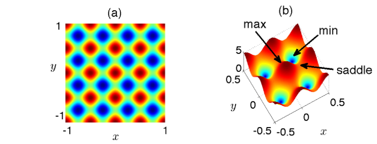
Figure 3: (Color online) The sinusoidal square lattice given by Eq. (19) with $V_{0}=5$. (a) Top view. (b) Side view. The solitons investigated below are centered at the lattice maximum (0,0), lattice minimum (0.25,0.25), and saddle point (0.25,0).

VIII.1 Solitons at lattice minima

We first investigate solitons centered at the lattice minimum $(x_{0},y_{0})=(0.25,0.25)$. Figure 4(a) shows that the power of solitons at lattice minima is below the critical power for collapse, i.e., $P(\mu)<P_{c}\approx 11.7$ for all $\mu$. As the soliton becomes narrower ($\mu\to-\infty$), the soliton power approaches $P_{c}$ from below (as was shown numerically in Musslimani and Yang (2004) for this lattice and analytically in Sivan et al. (2008a) for any linear lattice). In addition, as the soliton becomes wider ($\mu\to\mu^{(V)}_{BE}$, the edge of the first band), its power approaches $P_{c}$ from below (rather than becomes infinite, as implied in Musslimani and Yang (2004)), see also . The minimal power is obtained at $\mu=\mu_{m}\cong-10$. The power curve thus has a stable branch for narrow solitons ($-\infty<\mu<\mu_{m}$) where the slope condition is satisfied, and an unstable branch for wide solitons ($\mu_{m}<\mu<\mu^{(V)}_{BE}$) where the slope condition is violated. Therefore, wide solitons should be focusing-unstable while narrow solitons should be focusing-stable. Figure 4(b) shows that, as expected for solitons at lattice minima, $\lambda_{0}^{(1)}=\lambda_{0}^{(2)}>0$ for all $\mu$. Hence, the spectral condition is fulfilled. Consequently, solitons at lattice minima should not experience a drift instability.

In order to excite the focusing instability alone, we add to the soliton a small power perturbation, see Eq. (16). We contrast the dynamics in a neighborhood of stable and unstable solitons by choosing two solitons with the same power ($P\cong 0.98P_{c}$), from the stable branch ($\mu=-31$) and from the unstable branch ($\mu=-3$). We perturb these solitons with the same power perturbations ($c=0.5\%,1\%,2\%$).

When $c=0.5\%$ and $1\%$, the input power is below the threshold for collapse ($P<P_{c}$). In these cases, the self-focusing process is arrested and, during further propagation, the normalized peak intensity undergoes oscillations (see Figures 5(a) and (b)). For a given perturbation, the oscillations are significantly smaller for the stable soliton compared with the unstable soliton.

When $c=2.5\%$, the input power is above the threshold for collapse ($P>P_{c}$) and the solutions undergo collapse. Therefore, for such large perturbations, collapse occurs for both stable and unstable solitons, i.e., even when both the slope and spectral conditions are fulfilled. This shows yet again that in an inhomogeneous medium, collapse and instability are not necessarily correlated.

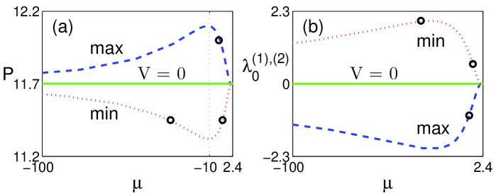
Figure 4: (Color online) (a) Power, and (b) perturbed-zero eigenvalues, as functions of the propagation constant, for solitons centered at a maximum (blue, dashes) and minimum (red, dots) of the lattice (19) with $V_{0}=5$. Also shown are the corresponding lines for the homogeneous NLS equation (solid, green). The circles (black) correspond to the values used in Figs. 5-8.

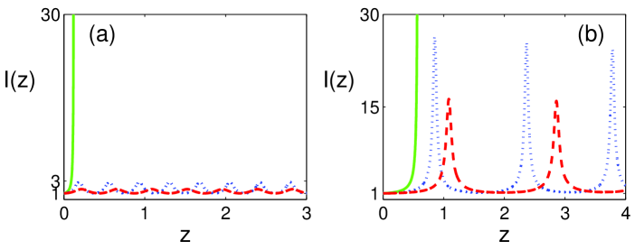
Figure 5: (Color online) Normalized peak intensity (18) of solutions of Eq. (15) with the periodic lattice (19) with $V_{0}=5$. Initial conditions are power-perturbed solitons [see Eq. (16)] centered at a lattice minimum: (a) Soliton from the stable branch ($\mu=-31$); (b) Soliton from the unstable branch ($\mu=-3$). Input powers are $0.5\%$ (red dots), $1\%$ (blue dashes), and $2.5\%$ (solid green) above the soliton power.

In order to confirm that solitons centered at a lattice minimum do not undergo a drift instability, we shift the soliton slightly upward by using the initial condition (17) with $(\Delta x_{0},\Delta y_{0})=(0,0.04)$. Under this perturbation, the solution of Eq. (10) is

$$\left\langle{x}\right\rangle\equiv 0,\quad\quad\left\langle{y}\right\rangle=\Delta y_{0}\cdot\cos(|\Omega_{y}|z).$$ (20)

In addition, by Eq. (12), $\Omega_{y}\approx 11.12i$ for $\mu=-31$ and $\Omega_{y}\approx 2.58i$ for $\mu=-3$. Figure 6(a1) shows that for $\mu=-31$, the center of mass in the $y$-direction of the position-shifted soliton follows the theoretical prediction (20) accurately over several oscillations. In addition, the center of mass in the $x$-direction remain at $x=0$ (data not shown), in agreement with Eq. (20). Thus, the soliton is indeed drift-stable.

The situation is more complex for $\mu=-3$. In this case, the position-shifted soliton follows the theoretical prediction (20) over more than $2$ diffraction lengths (i.e., for $z>z_{0}$ where $z_{0}\approx 1$), but then deviates from it, see Figure 6(b1). The reason for this instability is that for $\mu=-3$, the slope condition is violated. Since the position-shifted initial condition can also be viewed as an asymmetric amplitude power perturbation $\Delta A=u(x-\Delta x_{0},y-\Delta y_{0})-u(x,y)$, an focusing instability is excited and the soliton amplitude decreases (as its width increases), see Figure 6(b2). Obviously, once the soliton amplitude changes significantly, the theoretical prediction for the lateral dynamics is no longer valid. In order to be convinced that the initial instability in this case is of an focusing-type rather than drift-type, we note that for $\mu=-31$ for which the slope condition is satisfied, the soliton remains focusing-stable, see Figure 6(a2).

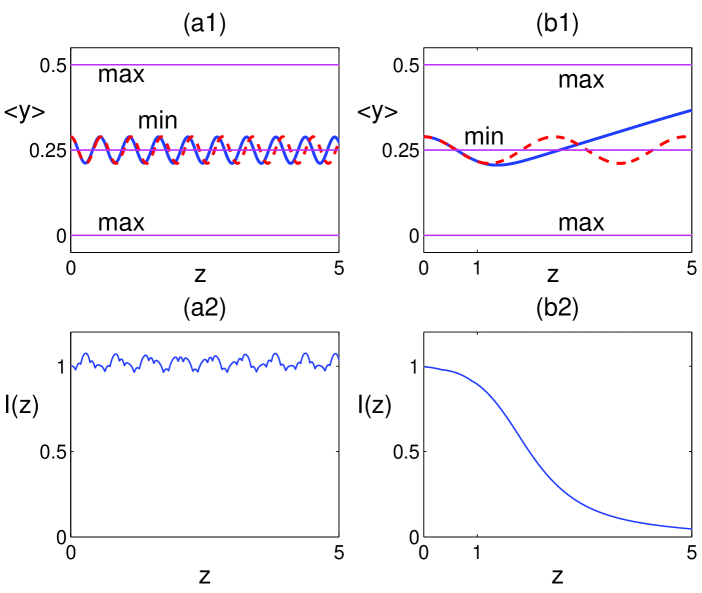
Figure 6: (Color online) Dynamics of solutions of Eq. (15) with the periodic lattice (19) with $V_{0}=5$. Initial conditions are position-shifted solitons [see Eq. (17)] centered at a lattice minimum, with $(\Delta x_{0},\Delta y_{0})=(0,0.04)$. (a1) Center of mass in the $y$ coordinate (blue, solid line) and analytical prediction [Eq. (20), red, dashes] for $\mu=-31$; (a2) Normalized peak intensity (18) for $\mu=-31$; (b1) and (b2) are the same as (a1) and (a2), but for $\mu=-3$.

VIII.2 Solitons at lattice maxima

We now investigate solitons centered at the lattice maximum $(x_{0},y_{0})=(0,0)$. Figure 4 shows that in general, solitons at lattice maxima have the opposite stability characteristics compared with those of solitons centered at lattice minima: The slope condition is violated for narrow solitons and satisfied for wide solitons, the power is above $P_{c}$ , and the perturbed-zero eigenvalues $\lambda_{0,j}^{(V)}$ are always negative. Interestingly, for the specific choice of the lattice (19), the powers and perturbed-zero eigenvalues at lattice maxima and minima are approximately, but not exactly, images of each other with respect to the case of a homogeneous medium.

The negativity of the perturbed-zero eigenvalues implies that solitons centered at a lattice maximum undergo a drift instability (see Figure 8(b)). However, if the initial condition is subject to a power perturbation, see Eq. (16), then no drift occurs. In this case, stability is determined by the slope condition. For example, Figure 7 shows the dynamics of a power-perturbed wide soliton for which the slope condition is satisfied. When the soliton’s input power is increased by $0.5\%$, the solution undergoes small focusing-defocusing oscillations, as in Figure 5(a), i.e., it is stable under symmetric perturbations. When the soliton’s input power is increased by $1\%$, the perturbation exceeds the “basin of stability” of the soliton Sivan et al. (2008a) and the soliton undergoes collapse. These results again demonstrate that collapse and instability are independent phenomena.

If the initial condition is asymmetric with respect to the lattice maximum, the soliton will undergo a drift instability. In Figure 8 we excite this instability with a small upward shift, namely, Eq. (17) with $(\Delta x_{0},\Delta y_{0})=(0,0.02)$. Under this perturbation, the solution of Eq. (10) is

$$\left\langle{x}\right\rangle\equiv 0,\quad\quad\left\langle{y}\right\rangle=\Delta y_{0}\cdot\cosh(\Omega_{y}z).$$ (21)

with $\Omega_{y}\approx 3.9$. In the initial stage of the propagation ($z<0.5$) the soliton drifts toward the lattice minimum – precisely following the asymptotic prediction (20), see Figure 8(a), but the soliton’s amplitude is almost constant), see Figure 8(b). During the second stage of the propagation ($0.5<z<0.99$) the soliton drifts somewhat beyond the lattice minimum as it begins to undergo self-focusing. In the final stage ($0.99<z<1$) the soliton undergoes collapse (Figure 8(b)). The global dynamics can be understood in terms of the stability conditions for solitons centered at lattice minima and maxima as follows. The initial soliton, which is centered at a lattice maximum, satisfies the slope condition but violates the spectral condition. Consistent with these traits, the soliton is focusing-stable but undergoes a drift instability. As the soliton gets closer to the lattice minimum, it can be viewed as a perturbed soliton centered at the lattice minimum, for which the spectral condition is fulfilled and the soliton power is below $P_{c}$ (see Figure 4(b)). Indeed, at this stage, the drift is arrested because the beam is being attracted back towards the lattice minimum. Moreover, the beam now is a strongly power-perturbed soliton, since the beam power ($\approx 1.03P_{c}$) is $\approx 6\%$ above the power of the soliton at a lattice minimum. Hence, in a similar manner to the results of Figure 5(a), the perturbation exceeds the “basin of stability” and the soliton undergoes collapse.

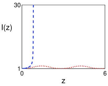
Figure 7: (Color online) Same as Figure 5(a) for a soliton at a lattice maximum with $\mu=-5$ (stable branch) and input power that is $0.5\%$ (red dots) and $1\%$ (blue dashes) above the soliton power.

Figure 8: (Color online) Dynamics of a soliton at a lattice maximum with $\mu=-5$, which is position-shifted according to (17) with $(\Delta x_{0},\Delta y_{0})\approx(0,0.02)$. (a) Center of mass in the $y$ coordinate (blue, dashes) and the analytical prediction (Eq. (21) with $\Omega_{y}\approx 3.9$, solid black). Location of lattice minimum and maxima are denoted by thin magenta and black horizontal lines, respectively. (b) Normalized peak intensity.

VIII.3 Solitons at a saddle point

From the didactic point of view, it is interesting also to consider solitons centered at a saddle point since they exhibit a combination of the features of solitons at lattice minima and maxima. To show this, we compute solitons centered at the saddle point $(x_{0},y_{0})=(0.25,0)$ of the lattice (19).

Figure 9(a) shows that the zero eigenvalues bifurcate into $\lambda_{0}^{(1)}>0$ on the stable $x$-direction, i.e., along direction in which the saddle is a minimum, and to $\lambda_{0}^{(2)}<0$ on the unstable $y$-direction, where the saddle in a maximum.

The opposite signs of the perturbed-zero eigenvalues imply a different dynamics in each of these directions. In order to excite only the drift instability, we solve Eq. (15) with $\mu=-12$ which belongs to the focusing-stable branch (see Figure 9(b2)). For this value of $\mu$, the perturbed zero eigenvalues are $\lambda_{0}^{(1)}\cong 1.7$ and $\lambda_{0}^{(2)}\cong-1.8$. By (12), the theoretical prediction for the oscillation period is $\Omega_{x}\cong|7i|=7$ whereas the drift rate is $\Omega_{y}\cong 7.2$. Hence, the theoretical prediction for the dynamics of the center of mass is

$$\left\langle{x}\right\rangle\approx 0.25+\Delta x_{0}\cdot\cos(7z),\quad\quad\left\langle{y}\right\rangle\approx\Delta y_{0}\cdot\cosh(7.2z).$$

Indeed, a shift in the $x$ direction $(\Delta x_{0},\Delta y_{0})\approx(0.0156,0)$ leads to oscillation in the $x$-direction (Figure 10(a)) while $\left\langle{y}\right\rangle$ (Figure 10(b)) and the amplitude (Figure 10(c)) are unchanged. On the other hand, a shift in the $y$ direction $(\Delta x_{0},\Delta y_{0})\approx(0,0.0156)$ leads to a drift instability in the $y$-direction (Figure 10(b)) but has no effect on $\left\langle{x}\right\rangle$ (Figure 10(a)). In both the stable and unstable directions, the center of mass follows the analytical prediction remarkably well. Figure 10(c) also shows that once the soliton drifts beyond the lattice minimum, the beam undergoes collapse. This can be understood using the same reasoning used for solitons that drift from a lattice maximum (see explanation for Figure 8 in Section VIII.2).

We also note that for the specific choice of the lattice (19), the values of the perturbed-zero eigenvalues in the stable and unstable directions are nearly indistinguishable from those of the perturbed-zero eigenvalues that correspond to solitons centered at a lattice minimum and maximum, respectively. This can be understood by rewriting the lattice (19) as

$$V(x,y)=\frac{V_{0}}{2}\left[1-\cos^{2}(2\pi(x-0.25))+\cos^{2}(2\pi y)\right].$$ (22)

Thus, apart from the constant part (i.e., the first term), the difference between the lattices is the sign before the $x$-component of the lattice. In that sense, in the $x$ direction, the saddle point is equivalent to a maximum point, hence, the similarity between the eigenvalues. Another consequence of the $x-y$ symmetry of the lattice (19) is that the soliton has approximately the critical power $P_{c}$ for all $\mu$, i.e., $P(\mu)\approx P_{c}$, which is approximately the average of the powers of solitons at maxima and minima (see Figure 9(b1,b2)). As noted before, this will be no longer true if the lattice changes in the $x$ and $y$ directions will no longer be equal.

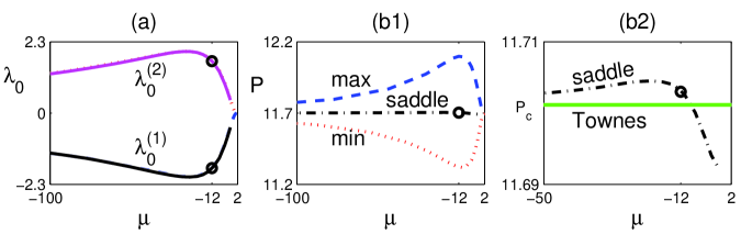
Figure 9: (Color online) (a) The perturbed-zero eigenvalues at the saddle point. One eigenvalue is shifted to positive values (magenta), and is indistinguishable from the eigenvalue at lattice minima (red); one eigenvalue is shifted to negative values (black), and is indistinguishable from the eigenvalue at lattice maxima (blue). (b1) Same data as in Figure 4(a), with the addition of data for solitons centered at a saddle point of the lattice (black, dash-dots). (b2) same as (b1) showing only the data for solitons centered at a saddle point (black, dash-dots) and for the homogeneous medium soliton (greed line).

Figure 10: (Color online) Dynamics of a soliton centered at a saddle point $(x_{0},y_{0})=(0.25,0)$ of the lattice (19) with $\mu=-12$ and shifts along: (i) the stable $x$ direction [$(\Delta x_{0},\Delta y_{0})\approx(0.0156,0)$, red dots], (ii) the unstable $y$ direction [$(\Delta x_{0},\Delta y_{0})\approx(0,0.0156)$, green dashes], (iii) the diagonal direction [$(\Delta x_{0},\Delta y_{0})\approx(0.0156,0.0156)$, blue, dash-dots]. (a) Center of mass $\left\langle{x}\right\rangle$. (b) Center of mass $\left\langle{y}\right\rangle$. (c) Normalized peak intensity.

If we apply perturbations in the stable and unstable directions simultaneously $(\Delta x_{0},\Delta y_{0})\approx(0.0156,0.0156)$, the dynamics in each coordinate is nearly identical to the dynamics when the perturbation was applied just in that direction. Thus, there is a “decoupling” between the (lateral dynamics in the) $x$ and $y$ directions. Indeed, this decoupling follows directly from Eq. (10).

VIII.4 Solitons at a shallow-maximum

We now consider solitons of the periodic potential

$$V(x,y)=\frac{V_{0}}{25}\left[2\cos(2\pi x)+2\cos(2\pi y)+1\right]^{2},$$ (23)

where $V_{0}=5$ and the normalization by $25$ implies that $V_{0}=\max_{x,y}V(x,y)$. Unlike the lattice (19), the lattice (23) also has shallow local maxima that are not global maxima [e.g., at (0.5,0.5)].

The stability and instability dynamics of solitons centered at global minima, maxima and saddle points of the lattice are similar to the case of the lattice (19), which was already studied. Hence, we focus only on the stability of solitons centered at a shallow maximum.

Since the lattice is invariant under a $90^{\circ}$ rotation, the perturbed-zero eigenvalues are equal, i.e., $\lambda_{0}^{(1)}=\lambda_{0}^{(2)}$. However, unlike solitons centered at a global maximum, the corresponding perturbed-zero eigenvalues are negative only for very negative values of $\mu$ (narrow beams) but become positive for values of $\mu$ near the band edge $\mu_{BE}$ (wide beams), see Figure 12(b). The reason for the positivity of $\lambda_{0}^{(1)}=\lambda_{0}^{(2)}$ despite being centered at a lattice maximum is as follows. For narrow solitons, the region where the “bulk of the beam” is located is of higher values of the potential compared with the immediate surrounding, hence, the solitons “feel” an effective lattice maximum. On the other hand, for wider solitons, the “bulk of the beam” is centered mostly at the shallow lattice maximum and the surrounding lower potential regions. Hence, although the very center of the soliton is at the shallow lattice maximum, these solitons are effectively centered at the lattice minimum with respect to the nearest global lattice maxima (see also Fibich et al. (2006), Section 4.5). The transition of the qualitative stability properties between narrow and wide solitons described above occurs when the soliton’s width is on the order of the lattice period. As noted in Section III.2, the stability at the transition points where $\lambda_{0,j}^{(V)}=0$ or $\frac{dP}{d\mu}=0$ requires a specific study. Similarly, a comparison of Figure 12(a) and Figure 4(a) shows that the $P(\mu)$ reflects the transition between properties which are characteristic to solitons centered at lattice maxima and minima. Indeed, for narrow solitons ($\mu\to-\infty$) is similar to the power of solitons centered at a global maximum, i.e., the power is above critical and the slope is positive. On the other hand, $P(\mu)$ curve for wide solitons ($\mu\to\mu^{(V)}_{BE}$) is similar to the power of solitons centered at a (simple) lattice minimum, i.e., the power is below critical and the slope is positive too.

Numerical simulations (Figure 13) demonstrate this transition. For a narrow soliton ($\mu=-12$), the theoretical prediction for the dynamics of the center of mass is $\left\langle{x}\right\rangle\cong 0.5+\Delta x_{0}\cosh(4.14z)$ and $\left\langle{y}\right\rangle\cong 0.5+\Delta y_{0}\cosh(4.14z)$. Indeed, the narrow soliton drifts away from the shallow maximum toward the nearby (global) lattice minimum (Figure 13(a1)) and then undergoes collapse (Figure 13(a2)). This dynamics is similar to that of solitons centered near lattice maximum or a saddle of a the lattice (19), see Sections VIII.2 and VIII.3. On the other hand, for the wide soliton ($\mu=-2$), the theoretical prediction for the dynamics of the center of mass is $\left\langle{x}\right\rangle\cong 0.5+\Delta x_{0}\cos(1.6z)$ and $\left\langle{y}\right\rangle\cong 0.5+\Delta y_{0}\cos(1.6z)$. Indeed, this soliton remains stable, undergoing small position oscillations around the shallow maximum (Figure 13(b)). This dynamics is the same as for solitons centered at a minimum of the lattice (19), see Figure 6(a). As in previous examples, the numerical results are in excellent agreement with the analytic prediction (10)-(12).

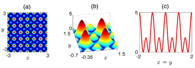
Figure 11: (Color online) The shallow maximum periodic lattice given by Eq. (23) with $V_{0}=5\,$. (a) Top view. (b) Side view. (c) Cross section along the line $x=y$.

Figure 12: (Color online) Same as Figure 4 for solitons centered at a shallow local maximum of the shallow-maximum periodic lattice (23).

Figure 13: (Color online) Dynamics of a perturbed soliton at shallow-maximum periodic lattice (23) with a narrow soliton [(a1) and (a2) with $\mu=-12$] and a wide soliton [(b) with $\mu=-2$], and using $(\Delta x_{0},\Delta y_{0})=(0.05,0.05)$. (a1) Center of mass $\left\langle{x}\right\rangle=\left\langle{y}\right\rangle$ of the narrow soliton (blue, dashes) and the analytical prediction (red dots). (a2) Normalized peak intensity of the narrow soliton. (b) Same as (a1) for the wide soliton.

IX Periodic lattices with defects

Defects play a very important role in energy propagation through inhomogeneous structures. They arise due to imperfections in natural or fabricated media. They are also often specifically designed to influence the propagation.

Solitons in periodic lattices with defects have drawn much attention both experimentally and theoretically; see, for example,  Ablowitz et al. (2006); Alfimov et al. (2002); Wang et al. (2007); Goodman-Slusher-Weinstein (2001). The complexity of the lattice details offers an opportunity to demonstrate the relative ease of applying the stability/dynamics criteria to predict and decipher the soliton dynamics in them. As an example, we study lattices with a point defect. Our analysis can also extend to different types of defects such as line defects, see e.g. Ablowitz et al. (2006).

We consider the lattice (23)

$$V(x,y)=\frac{V_{0}}{25}\left|2\cos(2\pi x)+2\cos(2\pi y)+e^{i\theta(x,y)}\right|^{2},$$ (24)

where the phase function $\theta(x,y)$ is given by

$$\theta(x,y)=\tan^{-1}\left(\frac{y-y_{0}}{x}\right)-\tan^{-1}\left(\frac{y+y_{0}}{x}\right),$$ (25)

see Figure 14 and also Ablowitz et al. (2006). Compared with the shallow-maximum periodic lattice (23), here the constant (DC) component (the third term in the lattice) attains a phase distortion which creates an (effective) vacancy defect at $(0,0)$, which is a shallow-maximum. Further, far away from the origin, the potential (24) is locally similar to the shallow-maximum periodic lattice (23). This is a generic example of a point defect, as opposed to a line defect Baba (2007). In what follows, we consider solitons centered at the vacancy defect $(x_{0},y_{0})=(0,0)$.

The stability properties of solitons in the shallow-maximum periodic (23) and vacancy-defect (24) lattices are strikingly similar, as can be seen from Figs. 12 and 15. In both cases, there is a marked transition between narrow and wide solitons and this transition occurs when the soliton width is of the order of the lattice period. Indeed, numerical simulations show that the dynamics of perturbed solitons is qualitatively similar in both cases – compare Figures 13 and 16. We do note that unlike the shallow-maximum periodic lattice, the perturbed-zero eigenvalues of the vacancy lattice bifurcate into different, though similar, values. The reason for this is the phase function (25) is not invariant by $90^{\circ}$ rotations.

Inspecting the lattice surfaces (Figures 11 and 14), it is clearly seen that the reason for the similarity between the shallow-maximum periodic and vacancy lattices is that the vacant site is essentially a shallow local maximum itself – and only a bit shallower than those of the shallow-maximum periodic lattice (see Figure 14).

In Figure 17 we give a detailed graphical illustration of a typical instability dynamics due to a violation of the spectral condition. Figure 17(a)-(c) show contours of the soliton profiles superposed on the contour plot of the lattice. It can be seen that as a result of the initial position shift, the soliton drifts towards the lattice minimum and that it self-focuses at the same time. Figure 17(d) shows the trajectory of the beam across the lattice. In addition, Figure 17(e) shows the center of mass dynamics as a function of the intensity $I(z)$. This shows that initially, the perturbed soliton undergoes a drift instability with little self-focusing, but that once the collapse accelerates, it is so fast so that the drift dynamics becomes negligible.

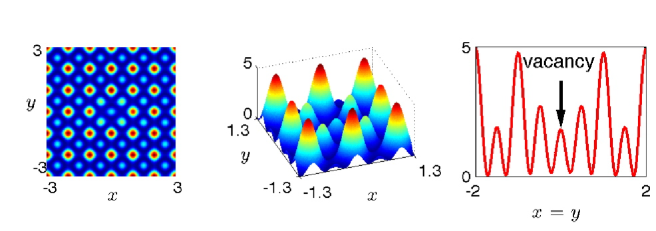
Figure 14: (Color online) Same as Figure 11 for solitons centered at the “vacancy” of the lattice (24).

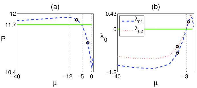
Figure 15: (Color online) Same as Figure 4 for solitons at the vacancy of the lattice (24). (b) The perturbed-zero eigenvalues $\lambda_{0}^{(1),(2)}$ are slightly different from each other. The circles (black) correspond to the values used in Figure 16.

Figure 16: (Color online) Same as Figure 13 but for the vacancy lattice (24). Here $\Omega_{x}\approx 3$ in (a2) and $\Omega_{x}\approx 1.09i$ in (b). In both cases the $\left\langle{y}\right\rangle$ dynamics (not shown) is similar (but not identical) to the $\left\langle{x}\right\rangle$ dynamics.

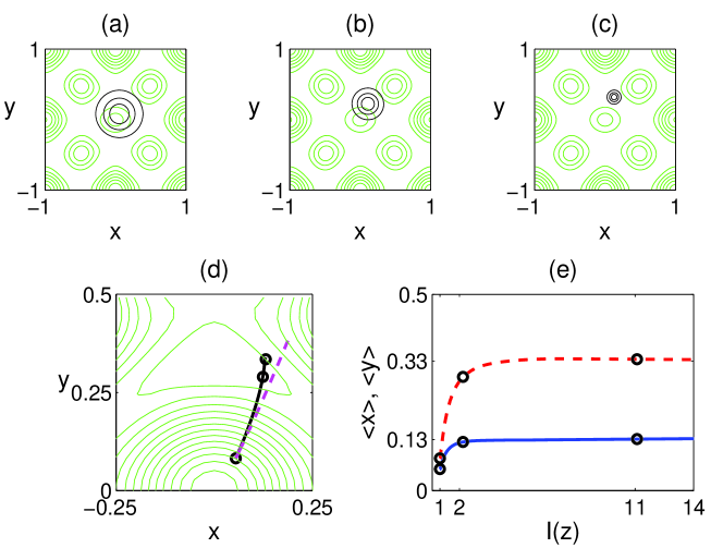
Figure 17: (Color online) (a)–(c): contours of the intensity $|u(x,y,z)|^{2}$ (blue) superimposed on the vacancy lattice (green) with initial conditions corresponding to the mode with $\mu=-8$ that is initially shifted in the $(x,y)$ plane to $(\Delta x_{0},\Delta y_{0})=(0.05,0.1)$, i.e., at an angle of $63^{o}$ to the $y$ axis. (a) $z=0,~{}I\approx 1$, (b) $z=0.51,~{}I\approx 2.18$, (c) $z=0.63,~{}I\approx 11.1$. (d) Center of mass dynamics (black curve) and the analytical prediction (magenta, dashes) superimposed on the contours of the potential (green). (e) $\left\langle{x}\right\rangle$ (blue, solid) and $\left\langle{y}\right\rangle$ (red, dashes) as functions of $I(z)$. Circles (black) correspond to the z-slices shown in (a)–(c).

X Quasicrystal lattices

Next, we investigate solitons in quasicrystal lattices. Such lattices appear naturally in certain molecules Shechtman et al. (1984); Marder (2001), have been investigated in optics Bratfalean et al. (2005); Lifshitz et al. (2005); Man et al. (2005); Freedman et al. (2006); Ablowitz et al. (2006) and in BEC Sanchez-Palencia and Santos (2005), and can be formed optically by the far-field diffraction pattern of a mask with point-apertures that are located on the $N$ vertices of a regular polygon, or equivalently, by the sum of $N$ plane waves (cf. Nye and Berry (1974); Ablowitz et al. (2006)) with wavevectors $(k_{x},k_{y})$ whose directions are equally distributed over the unit circle. The corresponding potential is given by

$$V(x,y)=\frac{V_{0}}{N^{2}}\left|\sum_{n=0}^{N-1}e^{i(k^{(n)}_{x}x+k^{(n)}_{y}y)}\right|^{2}~{},$$ (26)

where $(k^{(n)}_{x},k^{(n)}_{y})=\left(K\cos(2\pi n/N),K\sin(2\pi n/N)\right)$ . The normalization by $N^{2}$ implies that $V_{0}=\max_{x,y}V(x,y)$. The potential (26) with $N=2,3,4,6$ yields periodic lattices. All other values of $N$ correspond to quasicrystals, which have a local symmetry around the origin and long-range order, but, unlike periodic crystals, are not invariant under spatial translation Senechal (1995).

We first consider the case $N=5$ (a 5-fold symmetric “Penrose” quasicrystal) for solitons centered at the lattice maximum $(x_{0},y_{0})=(0,0)$, see Figure 18. Since the soliton profile and stability are affected mostly by the lattice landscape near its center, we can expect the stability properties of the Penrose lattice soliton at $(0,0)$ to be qualitatively the same as for a soliton at a lattice maximum of a periodic lattice. Indeed, Figure 19 reveals the typical stability properties of solitons centered at a lattice maximum: An focusing-unstable branch for narrow solitons, an focusing-stable branch for wider solitons and negative perturbed zero-eigenvalues (compare e.g. with Figure 8). Therefore, the Penrose soliton will drift from the lattice maximum under asymmetric perturbations and if the soliton is sufficiently narrow, it can also undergo collapse.

Figure 19 presents also the data for a perfectly periodic lattice ($N=4$) and for a higher-order quasicrystal ($N=11$). One can see that the stability properties in these lattices is qualitatively similar to the $N=5$ case. The only marked difference as $N$ increases is that the soliton’s power becomes larger for a given $\mu$.

These results show that in contrast to the significant effect of the quasi-periodicity on the dynamics of linear waves (compared with the effect of perfect periodicity Freedman et al. (2006)), the effect of quasi-periodicity on the dynamics of solitons is small.

Figure 18: (Color online) Same as Figure 11(a)+(b) for the Penrose quasicrystal lattice given by Eq. (26) with $N=5$ and $V_{0}=5$.

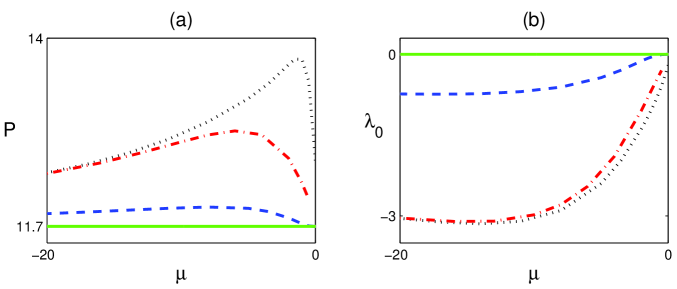
Figure 19: (Color online) Same as Figure 4 for solitons at the maxima of the lattices (26) with $N=4$ (periodic lattice, dashed blue line), $N=5$ (Penrose quasicrystal lattice, dash-dotted red line), $N=11$ (higher-order quasicrystal lattice, dotted black line), and the homogeneous NLS soliton (solid green line).

XI Single waveguide potentials

So far we studied periodic, periodic potentials with defects and quasiperiodic potentials. However, our theory can be applied to other types of potentials. Indeed, let us consider localized potentials, such as single or multiple waveguide potentials, for which the potential decays to zero at infinity. For such potentials, there are two limits of interest. The first limit is of solitons which are much wider than the width of the potential. In this case, the potential can be approximated as a point defect in an homogeneous medium. Then, the dynamics is governed by

$$iA_{z}(\vec{x},z)+\Delta A+|A|^{2\sigma}A-\gamma\delta(\vec{x})A=0,$$ (27)

where $\gamma$ is a real constant. In Le-Coz et al. (To appear), the qualitative and quantitative stability approaches were applied to Eq. (27) in one transverse dimension.

The second limit is of solitons which are much narrower than the width of the potential. In this case, only the local variation of the potential affects the soliton profile and stability. Hence, the potential can be expanded as

$$V(x)=V(0)+\frac{1}{2}V^{\prime\prime}(0)x^{2}+\cdots.$$

The qualitative and quantitative stability approaches were applied to this case in Sivan et al. (2008a).

In Le-Coz et al. (To appear); Sivan et al. (2008a), the profiles, power slope and perturbed-zero eigenvalues were computed analytically (exactly or asymptotically). It was proved that the perturbed-zero eigenvalues are negative for solitons centered at lattice maxima (repulsive potential) and are positive for solitons centered at lattice minima (attractive potential). Hence, in the latter case, stability is determined by the slope condition. In those two studies, detailed numerical simulations confirmed the validity of the qualitative and quantitative approaches. Hence, we do not present a systematic stability study for localized potentials.

XII Final remarks

In this paper, we presented a unified approach for analyzing the stability and instability dynamics of positive bright solitons. This approach consists of a qualitative characterization of the type of instability, and a quantitative estimation of the instability growth rate and the strength of stability. This approach was summarized by several rules (Section VI) and applied to a variety of numerical examples (Sections VIII-X), thus revealing the similarity between a variety of physical configurations which, a priori, look very different from each other. In that sense, our approach differs from most previous studies which considered a specific physical configuration.

One aspect which was emphasized in the numerical examples is the excellent agreement between direct numerical simulations of the NLS and the reduced equations for the center of mass (lateral) dynamics, Eqs. (10)-(12). Different reduced equations for the lateral dynamics were previously derived under the assumption that the beam remains close to the initial soliton profile (see e.g. Kartashov et al. (2004b)) or by allowing the soliton parameters to evolve with propagation distance (see e.g., Kivshar and Agrawal (2003) and references therein). These approaches, as well as ours, are valid only as long as the beam profile remains close to a soliton profile. However, unlike previous approaches, Eqs. (10)-(12) incorporate linear stability (spectral) information into the center of mass dynamics. Thus our approach shows that the beam profile evolves as a soliton perturbed by the eigenfunction $f_{0,j}^{(V)}$. The validity of this perturbation analysis is evident from the excellent comparison between the reduced Eqs. (10)-(12) and numerical simulations for a variety of lattice types. To the best of our knowledge, such an agreement was not achieved with the previous approaches.

The numerical examples in this paper were for two-dimensional Kerr media with various linear lattices. Together with our previous studies which were done for narrow solitons in any dimension Sivan et al. (2008a), a linear delta-function potential Le-Coz et al. (To appear) and for nonlinear lattices Fibich et al. (2006); Sivan et al. (2006), there is a strong numerical evidence that our qualitative and quantitative approaches apply to positive solitons in any dimension, any type of nonlinearity of type $F(|A|^{2})$ (e.g., saturable) as well as for other lattice configurations, e.g., “surface” or “corner” solitons Makris et al. (2005).

Theorem III.1 as well as the qualitative and quantitative approaches apply also for the $d$-dimensional discrete NLS. This equation is obtained from Eq. (15) by replacing $\Delta$ by the difference Laplacian operator on a discrete lattice and $V$ by a potential defined at discrete lattice sites. This model was extensively studied, mostly for periodic lattices, see e.g., for 1D and 2D discrete NLS equation with cubic nonlinearity (see e.g., Christodoulides and Joseph (2008); Eisenberg et al. (1998); Efremidis et al. (2002); Christodoulides et al. (2003); Fleischer et al. (2003); Sukhorukov et al. (2003)), saturable nonlinearity (see e.g., discrete_NLS_saturable ), cubic-quintic nonlinearity (see e.g., Malomed-discrete-cq ). General results on existence and stability of solitons in $d-$ dimensions with power nonlinearities appear in Weinstein-Discrete (1999); Weinstein-discrete . Indeed, for the discrete NLS, the operator $L_{+}$ does not generically have a zero eigenvalue due to absence of continuous translation symmetry, and the continuous spectrum is a bounded interval, starting at the soliton frequency, $-\mu$ Weinstein-discrete . However, these changes in the spectrum do not affect the stability theory, the possible types of instabilities and the analysis of their strength.

As noted, our analysis shows that for positive bright solitons, only two types of instabilities are possible - focusing instability or drift instability. Other types of instabilities may appear, but only for non-positive solitons (e.g., gap solitons or vortex solitons). A formulation of a qualitative and quantitative theories for such solitons requires further study.

References

- Eisenberg et al. (1998) H. Eisenberg, Y. Silberberg, R. Morandotti, A. Boyd, and J. Aitchison, Phys. Rev. Lett. 81, 3383 (1998).
- Efremidis et al. (2002) N. Efremidis, D. Christodoulides, S. Sears, J. Fleischer, and M. Segev, Phys. Rev. E 66, 046602 (2002).
- Fleischer et al. (2003) J. Fleischer, M. Segev, N. Efremidis, and D. Christodoulides, Nature 422, 147 (2003).
- Christodoulides et al. (2003) D. Christodoulides, F. Lederer, and Y. Silberberg, Nature 424, 817 (2003).
- Sukhorukov et al. (2003) A. Sukhorukov, Y. Kivshar, H. Eisenberg, and Y. Silberberg, IEEE J. Quant. Elec. 39, 31 (2003).
- Efremidis et al. (2003) N. Efremidis, J. Hudock, D. Christodoulides, J. Fleischer, O. Cohen, and M. Segev, Phys. Rev. Lett. 91, 213906 (2003).
- Neshev et al. (2004) D. Neshev, Y. Kivshar, H. Martin, and Z. Chen, Opt. Lett. 29, 486 (2004).
- Pertsch et al. (2004) T. Pertsch, U. Peschel, J. Kobelke, K. Schuster, H. Bartelt, S. Nolte, A. Tünnermann, and F. Lederer, Phys. Rev. Lett. 93, 053901 (2004).
- Carr et al. (2001) L. Carr, K. Mahmud, and W. Reinhardt, Phys. Rev. A 64, 033603 (2001).
- Linzon et al. (2007) Y. Linzon, R. Morandotti, M. Volatier, V. Aimez, R. Ares, and S. Bar-Ad, Phys. Rev. Lett. 99, 133901 (2007).
- Sakaguchi and Tamura (2004) H. Sakaguchi and M. Tamura, J. Phys. Soc. Jap. 73, 503 (2004).
- Makris et al. (2005) K. Makris, S. Suntsov, D. Christodoulides, G. Stegeman, and A. Hache, Opt. Lett. 30, 2466 (2005).
- Kartashov et al. (2004a) Y. Kartashov, V. Vysloukh, and L. Torner, Phys. Rev. Lett. 93, 093904 (2004a).
- Kevrekidis et al. (2002) P. Kevrekidis, B. Malomed, and Y. Gaididei, Phys. Rev. E 66, 016609 (2002).
- Rosberg et al. (2007) C. Rosberg, D. Neshev, A. Sukhorukov, W. Krolikowski, and Y. Kivshar, Opt. Lett. 32, 397 (2007).
- Ablowitz et al. (2006) M. Ablowitz, B. Ilan, E. Schonbrun, and R. Piestun, Phys. Rev. E - Rap. Comm. 74, 035601 (2006).
- Fedele et al. (2005) F. Fedele, J. Yang, and Z. Chen, Stud. Appl. Math. 115, 279 (2005).
- Makasyuk and Chen (2006) I. Makasyuk and Z. Chen, Phys. Rev. Lett. 96, 223903 (2006).
- Martin et al. (2004) H. Martin, E. Eugenieva, Z. Chen, and D. Christodoulides, Phys. Rev. Lett. 92, 123902 (2004).
- Qi et al. (2004) M. Qi, E. Lidorikis, P. Rakich, S. Johnson, J. Joannopoulos, E. Ippen, and H. Smith, Nature 429, 538 (2004).
- Ryu et al. (2003) H. Y. Ryu, S. H. Kim, H. G. Park, and Y. H. Lee, J. Appl. Phys. 93, 831 (2003).
- Yang and Chen (2006) J. Yang and Z. Chen, Phys. Rev. E 73, 026609 (2006).
- Bratfalean et al. (2005) R. Bratfalean, A. Peacock, N. Broderick, K. Gallo, and R. Lewen, Opt. Lett. 30, 424 (2005).
- Freedman et al. (2006) B. Freedman, G. Bartal, M. Segev, R. Lifshitz, D. Christodoulides, and J. Fleischer, Nature 440, 1166 (2006).
- Lifshitz et al. (2005) R. Lifshitz, A. Arie, and A. Bahabad, Phys. Rev. Lett. 95, 133901 (2005).
- Man et al. (2005) W. Man, M. Megens, P. Steinhardt, and P. Chaikin, Nature 436, 993 (2005).
- Villa et al. (2005) A. D. Villa, S. Enoch, G. Tayeb, V. Pierro, V. Galdi, and F. Capolino, Phys. Rev. Lett. 94, 183903 (2005).
- Xie et al. (2003) P. Xie, Z.-Q. Zhang, and X. Zhang, Phys. Rev. E 67, 026607 (2003).
- Schwartz et al. (2007) T. Schwartz, G. Bartal, S. Fishman, and M. Segev, Nature 446, 52 (2007).
- Lahini et al. (2008) Y. Lahini, A. Avidan, F. Pozzi, M. Sorel, R. Morandotti, D. Christodoulides, and Y. Silberberg, Phys. Rev. Lett. 100, 013906 (2008).
- Abdullaev et al. (2005) F. Abdullaev, A. Gammal, A. Kamchatnov, and L. Tomio, Int. J. of Mod. Phys. B 19, 3415 (2005).
- Konotop (2005) V. Konotop, in Dissipative Solitons ed. N. Akhmediev (Springer, 2005).
- Fibich et al. (2006) G. Fibich, Y. Sivan, and M.I. Weinstein, Physica D 217, 31 (2006).
- Sivan et al. (2006) Y. Sivan, G. Fibich, and M.I. Weinstein, Phys. Rev. Lett. 97, 193902 (2006).
- Sivan et al. (2008a) Y. Sivan, G. Fibich, N. Efremidis, and S. Barad, Nonlinearity 21, 509 (2008a).
- Le-Coz et al. (To appear) S. Le-Coz, R. Fukuizumi, G. Fibich, B. Ksherim, and Y. Sivan, Physica D 237, 1103 (To appear).
- Sivan et al. (2008b) Y. Sivan, G. Fibich, and B. Ilan, Phys. Rev. E(R) 77, 045601(R) (2008b).
- (38) B. Crosignani, P. DiPorto, M. Segev, G. Salamo, and A. Yariv, Nonlinear optical beam propagation and solitons in photorefractive media, La Rivista del Nuovo Cimento 21 (1998), 1.
- Pethick and Smith (2001) C. Pethick and H. Smith, Bose-Einstein Condensation in Dilute Gases (Cambridge University Press, 2001).
- Musslimani and Yang (2004) Z. Musslimani and J. Yang, J. Opt. Soc. Am. B 21, 973 (2004).
- Vakhitov and Kolokolov (1973) M. Vakhitov and A. Kolokolov, Radiophys. Quant. Elec. 16, 783 (1973).
- Cazenave and Lions (1982) T. Cazenave and P.-L. Lions, Comm. Math. Phys. 85, 549 (1982).
- Weinstein (1986) M.I. Weinstein, Comm. Pure Appl. Math. 39, 51 (1986).
- Grillakis et al. (1987) M. Grillakis, J. Shatah, and W. Strauss, J. Funct. Anal. 74, 160 (1987).
- Grillakis et al. (1990) M. Grillakis, J. Shatah, and W. Strauss, J. Funct. Anal. 94, 308 (1990).
- (46) N. Akhmediev, A. Ankiewicz, R. Grimshaw, Phys. Rev. E 59, 6088 (1999).
- Rose and Weinstein (1988) H. Rose and M.I. Weinstein, Physica D 30, 207 (1988).
- Weinstein (1989) M.I. Weinstein, Contemp. Math. 99, 213 (1989).
- Oh (1989) Y.-G. Oh, Comm. Math. Phys.. 121, 11 (1989).
- Grillakis (1988) M. Grillakis, Comm. Pure Appl. Math. 41, 747-774 (1988).
- Jones (1988) C.K.R.T. Jones, J. Diff. Eqns. 71, 34-62 (1988).
- Comech and Pelinovsky (2003) A. Comech and D. Pelinovsky Comm. Pure Appl. Math. 56, 1565-1607 (2003); J. Marzuola, Ph.D. thesis, U.C. Berkeley (2007)
- (53) B. Ilan and M.I. Weinstein, in preparation.
- Sulem and Sulem (1999) C. Sulem and P. L. Sulem, The Nonlinear Schrödinger Equation (Springer, 1999).
- Weinstein (1985) M.I. Weinstein, SIAM J. Math. Anal. 16, 472 (1985).
- Mihalache et al. (2005) D. Mihalache, D. Mazilu, F. Lederer, B. Malomed, L.-C. Crasovan, Y. Kartashov, and L. Torner, Phys. Rev. A 72, 021601 (2005).
- Mihalache et al. (2004) D. Mihalache, D. Mazilu, F. Lederer, B. Malomed, L.-C. Crasovan, Y. Kartashov, and L. Torner, Phys. Rev. E 70, 055603(R) (2004).
- Pelinovsky et al. (2004) D. Pelinovsky, A. Sukhorukov, and Y. Kivshar, Phys. Rev. E 70, 036618 (2004).
- Rapti et al. (2007) Z. Rapti, P. Kevrekidis, V. Konotop, and C. Jones, J. Phys. A. 40, 14151 (2007).
- Lin and Wei (To appear) T. Lin and J. Wei, SIAM J. Math. Anal. (To appear).
- Weinstein (1983) M.I. Weinstein, Comm. Math. Phys. 87, 567 (1983).
- Fibich and Merle (2001) G. Fibich and F. Merle, Physica D 155, 132 (2001).
- Gisin et al. (2004) B. Gisin, R. Driben, and B. Malomed, J. Opt. B 6, S259 (2004).
- Ablowitz and Musslimani (2005) M. Ablowitz and Z. Musslimani, Opt. Lett. 30, 2140 (2005).
- Cristiani et al. (2002) M. Cristiani, O. Morsch, J. Müller, D. Ciampini, and E. Arimondo, Phys. Rev. A 65, 063612 (2002).
- Jona-Lasinio et al. (2003) M. Jona-Lasinio, O. Morsch, M. Cristiani, N. Malossi, J. Müller, E. Courtade, M. Anderlini, and E. Arimondo, Phys. Rev. Lett. 91, 230406 (2003).
- Alfimov et al. (2002) G. Alfimov, P. Kevrekidis, V. Konotop, and M. Salerno, Phys. Rev. E 66, 046608 (2002).
- Wang et al. (2007) J. Wang, J. Yang, and Z. Chen, Phys. Rev. A 76, 013828 (2007).
- Baba (2007) T. Baba, Nature Photonics 1, 11 (2007).
- Shechtman et al. (1984) D. Shechtman, I. Blech, D. Gratias, and J. W. Cahn, Phys. Rev. Lett. 53, 1951 (1984).
- Marder (2001) M. P. Marder, Condensed Matter Physics (Wiley-Interscience, 2001).
- Sanchez-Palencia and Santos (2005) L. Sanchez-Palencia and L. Santos, Phys. Rev. A 72, 053607 (2005).
- Nye and Berry (1974) J. Nye and M. Berry, Proc. Royal Soc. London 336, 165 (1974).
- Senechal (1995) M. Senechal, Quasicrystals and Geometry (Cambridge University Press, 1995).
- Kartashov et al. (2004b) Y. Kartashov, A. Zelenina, L. Torner, and V. Vysloukh, Opt. Lett. 29, 766 (2004b).
- Kivshar and Agrawal (2003) Y. Kivshar and G. Agrawal, Optical Solitons (Academic Press, 2003).
- Soffer-Weinstein (2004) A. Soffer and M.I. Weinstein, Rev. Math. Phys. 16, 977 (2004).
- Soffer-Weinstein (2005) A. Soffer and M.I. Weinstein, Phys. Rev. Lett. 95, 213905 (2005).
- Goodman-Slusher-Weinstein (2001) R.H. Goodman and R.E. Slusher and M.I. Weinstein J. Opt. Soc. Am. B 19, 1635-1652 (2001).
- Kupper-Stuart (1990) T. Kupper and C.A. Stuart J. Reine Ang. Math. 409, 1-34 (1990).
- Kirr and Kevrekides and Shlizerman and Weinstein (2008) E. Kirr, P. Kevrekidis, E. Shlizerman and M.I. Weinstein, http://arxiv.org/pdf/nlin/0702038, SIAM J. Math. Analysis, in press.
- Weinstein-Discrete (1999) M.I. Weinstein, Nonlinearity, 12, 673–691 (1999)
- Christodoulides and Joseph (2008) D.N. Christodoulides, R.I. Joseph, Opt. Lett. 13, 794 (1988)
- (84) L. Hadz̆ievski et al., Phys. Rev. Lett. 93, 033901 (2004). R. Vicencio and M. Johansson, Phys. Rev. E 73, 046602 (2006).
- (85) R. Carretero-Gonzalez, J.D., Talley, C. Chong and B.A. Malomed, Physica D 216, 77 (2006).
- (86) M.I. Weinstein and B. Yeary, Phys. Lett. A 222, 157 (1996). B.A. Malomed and M.I. Weinstein, Phys. Lett. A 220, 91 (1996).
- (87) B. Ilan, Y. Sivan and M.I. Weinstein, Preprint.