Cytoskeleton mediated effective elastic properties of model red blood cell membranes

Abstract

The plasma membrane of human red blood cells consists of a lipid bilayer attached to a regular network of underlying cytoskeletal polymers. We model this system at a dynamic coarse-grained level, treating the bilayer as an elastic sheet and the cytoskeletal network as a series of phantom entropic springs. In contrast to prior simulation efforts, we explicitly account for dynamics of the cytoskeletal network, both via motion of the protein anchors that attach the cytoskeleton to the bilayer and through breaking and reconnection of individual cytoskeletal filaments. Simulation results are explained in the context of a simple mean-field percolation model and comparison is made to experimental measurements of red blood cell fluctuation amplitudes.

I Introduction

Membranes are essential components of all biological cells Alberts et al. (2002). In addition to their biological importance, lipid bilayers and biomembranes have also attracted considerable attention from physicists due to their fascinating and unusual properties Safran (2003); Gre (1995). One particularly well studied system is the human red blood cell (RBC) membrane. The RBC membrane is a composite structure, consisting of a lipid bilayer adhered to an underlying network of filamentous cytoskeletal proteins (spectrin) via integral membrane protein anchors (see Fig. 1). The spectrin network is observed to be quite regular Liu et al. (1987), with an approximate hexagonal symmetry extending over the entire cell surface. (It is worth emphasizing that the spectrin based cytoskeletal network of RBCs is completely different from the three dimensional actin networks common to other types of animal cells Alberts et al. (2002).)

Given the apparent simplicity of the RBC membrane, it is tempting to attempt modeling with elementary elastic models. Indeed, there is a rich history of elastic RBC models to be found in the literature Brochard and Lennon (1975); Peterson (1992); Gov et al. (2003); Lim et al. (2002); Fournier et al. (2004); Rochal and Lorman (2006). Without attempting a full historical review here, we comment that no single elastic model has yet been identified that is capable of reproducing the full set of experimental data available for RBC membranes. For example, while the work of Lim, Wortis and Mukhopadhyay Lim et al. (2002) is capable of capturing the range of observed RBC shapes (stomatocyte, discocyte, echinocyte and non-main-sequence shapes as well) seen under various chemically induced stresses (e.g. pH, salt, ATP, etc.), this model has not been applied to explain the thermal fluctuation amplitudes observed in RBC membranes. And, while the models of Gov, Zilman and Safran Gov et al. (2003) and Fournier, Lacoste and Raphael Fournier et al. (2004) appear to do a good job fitting thermal fluctuation data Zilker et al. (1987), these models do not appear capable of explaining mechanical deformation experiments on RBCs Discher et al. (1994); Heinrich et al. (2001); Engelhardt et al. (1984). The failure of simple models to consistently explain both thermal fluctuations and mechanical deformation experiments has been recognized for years Peterson (1992). One recent model does explain both types of data within a single elastic model Rochal and Lorman (2006), however this model treats the spectrin network as an incompressible and homogeneous viscoelastic plate coupled to the lipid bilayer. It remains unclear why such an approximation should suffice for the sparse cytoskeletal network present in RBCs. Additionally, this model seems too simplistic to capture the full range of shape behaviors explained in reference Lim et al. (2002).

The models mentioned in the preceding paragraph make no mention of the role of energy expenditure in the behavior of RBC membranes. This despite the fact that it is known that RBC membranes possess kinase and phosphatase activities capable of altering the properties of spectrin and other network associated proteins via (de)phosphorylation Birchmeier and Singer (1977); Bennett (1989). And, certain measurements of RBC fluctuation amplitudes show a correlation between ATP concentration and fluctuation magnitude Levin and Korenstein (1991); Tuvia et al. (1998). One might argue that the difficulty in fitting all RBC behavior to a single elastic model stems from the fact that a truly comprehensive model must incorporate the effects of energy expenditure by the cell in a realistic fashion. Gov and Safran Gov and Safran (2005) are the first to seriously consider active energy expenditure within the RBC from a theoretical standpoint. They have proposed that ATP induced phosphorylation and dephosphorylation of the RBC cytoskeletal network leads to a continual dynamic evolution of the integrity of the spectrin network. While this picture remains hypothetical, without direct proof, it is consistent with the general observations relating ATP concentration to membrane fluctuation amplitudes. Gov and Safran (GS) Gov and Safran (2005) have used this picture to motivate a simple picture for RBC fluctuations under the presence of ATP. Local breaking and reforming of the spectrin network is captured via non-thermal forces imparted on an elastic membrane model. This model has provided the first plausible explanation for the viscosity dependence of RBC fluctuations Tuvia et al. (1997).

While elastic models with proper accounting for non-thermal energetics may eventually prove adequate in describing the long wavelength physics of the RBC, it is clear that wavelengths near or below the spectrin mesh size ($\sim 100nm$) must be considered within a more microscopic picture. A recent model by Dubus and Fournier (DF) Dubus and Fournier (2006) has extended the traditional elastic modeling of RBC membranes to explicitly include the cytoskeletal network at a molecular level of detail. Within this model, the spectrin network is considered as a completely regular hexagonal network of phantom entropic springs attached to a fluid lipid bilayer. Over wavelengths significantly longer that the spectrin mesh size, the network so modeled becomes mathematically equivalent to an imposed surface tension on the fluid bilayer. At wavelengths comparable to and shorter than network spacing, the system behaves differently from a simple membrane with applied tension. This model was used to compute the spectrum of thermal fluctuation amplitudes for the RBC membrane, but made no attempt to account for non-thermal consumption of energy and only computed thermal (non-dynamic) observables.

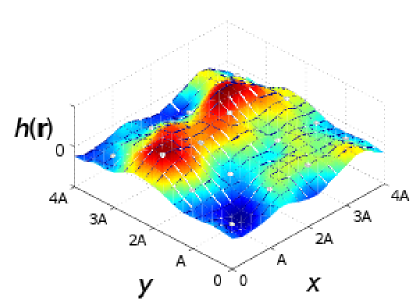
Figure 2: (Color online). A snapshot the RBC membrane as treated in our simulations. The lipid bilayer is connected to spectrin via a series of laterally mobile anchoring proteins (white dots). The anchors are interconnected via harmonic potentials (not shown for clarity), modeling the entire cytoskeletal network as a series of interconnected entropic springs. Our model does not account for any steric repulsion between cytoskeleton and bilayer surface, nor does it account for inextensibility of spectrin beyond its natural contour length; the individual spectrin links are treated as simple Gaussian chains. Individual links in the network are allowed to break and reform following kinetic equations that do not obey detailed balance; this provides a model for energy (ATP) consumption at the membrane surface. $A$ is the average mesh size ($\sim 100nm$).

In this paper, we extend the DF entropic spring model of the cytoskeleton meshwork to include dynamic evolution of the entire system. We allow the anchor points between spectrin and membrane to laterally diffuse and we allow for dynamic dissociation and association of spectrin links as a molecular level manifestation of the non-thermal energetic picture proposed by GS (fig. 2).

One important consequence of the GS picture is that sufficiently high ATP concentrations lead to an appreciable fraction of dissociated spectrin links at the membrane surface. Depending upon the timescales for spectrin (re)association, the effective long-wavelength elastic properties of the membrane interpolate between two limiting cases. If spectrin (re)association kinetics are much slower than all other timescales in the problem, the effective tension imposed by the network (as inferred by out-of-plane bilayer undulations) is well predicted by a simple percolation-theory argument (see fig. 3). In the opposite limit of fast spectrin kinetics, the effective tension is well predicted by assuming each link in the network has a reduced spring constant proportional to the probability of the link being intact at steady state. At intermediate rates, simulations are seen to interpolate between the two extreme cases.

This paper is organized as follows. In Sec. II, we present our mathematical model for the RBC membrane. In Sec. III details of our simulation methods are discussed. In Sec. IV results for a fully intact spectrin meshwork are presented, while in Sec. V we generalize to the more interesting case of a randomly broken network (both static and dynamically broken). We discuss our results in relation to experiment in Sec. VI and conclude in Sec. VII.

II Model

We treat the RBC membrane as a Helfrich fluid sheet Helfrich (1973) coupled via mobile anchor points to a network of springs. Our Hamiltonian is

$$H = \int_{\mathcal{A}}d\mathbf{r}\frac{\kappa}{2}[\nabla^{2}h(\mathbf{r})]^{2}$$

$$+ \sum_{\langle i,j\rangle}\xi_{ij}(t)\left\{\frac{\mu}{2}(\mathbf{r}_{i}-\mathbf{r}_{j})^{2}+\frac{\mu}{2}[h(\mathbf{r}_{i})-h(\mathbf{r}_{j})]^{2}+E\right\}.$$

The first term (integral portion) is the standard bilayer bending energy for a Monge gauge sheet assuming small deformations Helfrich (1973) and bending modulus $\kappa$. $\mathcal{A}$ is the projected area of the membrane, $\mathbf{r}=(x,y)$ is the position vector in the $xy$ plane and and $h(\mathbf{r})$ is the local displacement of the membrane away from the flat reference configuration specified by $h(\mathbf{r})=0$ (see Fig. 2). We assume that the lipid bilayer itself has a negligible (bare) surface tension. In more general situations, eq. LABEL:eq:H is easily modified to account for non-vanishing tension inherent to the lipid bilayer portion of the membrane Safran (2003); Helfrich (1973). The second term (sum portion) accounts for the energy of the 2D cytoskeletal meshwork, modelled as a network of entropic springs (or in other words, ideal chains of polymers) with effective spring constant $\mu$ ($\mu=3k_{B}T/\ell_{k}\ell_{c}$ with $\ell_{k}$ and $\ell_{c}$ the Kuhn and contour length of the polymer, respectively). In a fully intact cytoskeletal meshwork, all spring end points (nodes) are restricted to lie on the surface of the bilayer, so their coordinates are specified by $\mathbf{r_{i}}$ and $h(\mathbf{r_{i}})$, with indices $i$ (or $j$) labelling different nodes. The sum is over all distinct nearest neighbor node pairs (equivalently, over all polymer springs), denoted as $\langle i,j\rangle$. The factor $\xi_{ij}(t)$ is included to account for the possibly incomplete connectivity of the network. It is equal to 1 when the $ij$ link is connected and 0 otherwise. The constant $E$ reflects all other free energy change associated with connecting a detached filament end to a node besides the elastic energy of the spring (e.g., the binding energy to the node); we assume this energy is negative and significantly larger than thermal energy scales to insure stability of the network in the absence of non-thermal energy sources.

Although our starting point is very similar to the DF model, we emphasize a few key differences. In DF, the lateral positions of nodes are held fixed in the geometry of minimum energy for a flat bilayer surface; i.e. the $r_{i}$ variables are treated as set constants in DF, not as variables capable of influencing the energetics and/or dynamics of the system. This approximation renders the Hamiltonian analytically tractable, however it is not immediately clear that such a choice fully captures all relevant physics in this system. For example, with fixed node positions equally spaced on a regular lattice, the “spring” contribution to eq. LABEL:eq:H amounts to a finite differenced version of the usual surface tension contribution to the Helfrich Hamiltonian. At long wavelengths, eq. LABEL:eq:H with fixed nodes is guaranteed to behave as a Helfrich sheet under tension. If the nodes are mobile, as physically expected, the spring network represents a simple manifestation a tethered membrane. Such membranes are known to exhibit more complicated fluctuations than expected for Helfrich fluid bilayers Nelson and Peliti (1987). We also emphasize that much of the following work is concerned with membrane dynamics, which was not considered in DF. One of the most interesting aspects of our model is the dynamic breaking and reformation of cytoskeletal filaments, which could not be studied with the equilibrium approach adopted by DF.

Dynamics in our system are overdamped, owing to the low Reynolds number environment present at cellular length scales Purcell (1977). For bilayer height fluctuations, we have the following Langevin type equation of motion, which accounts for hydrodynamic flow in the surrounding cytoplasm  Granek (1997); Lin and Brown (2005); Brown (2008)

$$\frac{\partial h(\mathbf{r},t)}{\partial t}=\int_{-\infty}^{\infty}d\mathbf{r}^{\prime}\Lambda(\mathbf{r}-\mathbf{r}^{\prime})[F(\mathbf{r}^{\prime},t)+\zeta(\mathbf{r}^{\prime},t)].$$ (2)

Here, $\Lambda(\mathbf{r})$ is the diagonal part of the Oseen tensor Doi and Edwards (1986), given by

$$\Lambda(\mathbf{r})=\frac{1}{8\pi\eta|\mathbf{r}|},$$ (3)

where $\eta$ is the viscosity of the surrounding fluid. The above integral is taken over the entire $x,y$ plane; it is assumed that the area of interest, $\mathcal{A}$, is embedded within a periodically repeating environment of identical subsystems. $F(\mathbf{r},t)$ is the force per unit area on the membrane,

$$F(\mathbf{r},t) = -\frac{\delta H}{\delta h(\mathbf{r},t)}=-\kappa\nabla^{4}h(\mathbf{r},t)$$ (4)

$$- \sum_{\langle j\rangle}\mu\xi_{ij}(t)\delta^{2}(\mathbf{r-r}_{i})[h(\mathbf{r},t)-h(\mathbf{r}_{j},t)],$$

where $\delta(\mathbf{r})$ is the Dirac delta function, and the sum is over all nearest neighbors of node $i$, denoted as $\langle j\rangle$. $\zeta(\mathbf{r},t)$ is a spatially local Gaussian white noise satisfying the fluctuation-dissipation relation

$$\langle\zeta(\mathbf{r},t)\rangle = 0,$$ (5)

$$\langle\zeta(\mathbf{r},t)\zeta(\mathbf{r}^{\prime},t^{\prime})\rangle = 2k_{B}T\Lambda^{-1}(\mathbf{r-r^{\prime}})\delta(t-t^{\prime}),$$ (6)

where $k_{B}$ is Boltzmann’s constant and $T$ temperature of the system.

We have another set of Langevin equations describing lateral diffusion of the nodes within the bilayer

$$\frac{\partial\mathbf{r}_{i}(t)}{\partial t}=\frac{D}{k_{B}T}[\mathbf{F}_{i}(t)+\boldsymbol{\zeta}_{i}(t)],$$ (7)

with

$$\mathbf{F}_{i}(t) = -\frac{\partial H}{\partial\mathbf{r}_{i}}$$

$$= -\sum_{\langle j\rangle}\mu\xi_{ij}(t)\left\{(\mathbf{r}_{i}-\mathbf{r}_{j})+[h(\mathbf{r}_{i})-h(\mathbf{r}_{j})]\frac{\partial h(\mathbf{r}_{i})}{\partial\mathbf{r}_{i}}\right\},$$

and

$$\langle\boldsymbol{\zeta}_{i}(t)\rangle = 0,$$ (9)

$$\langle\boldsymbol{\zeta}_{i}(t)\cdot\boldsymbol{\zeta}_{j}(t^{\prime})\rangle = \frac{4(k_{B}T)^{2}}{D}\delta_{ij}\delta(t-t^{\prime}),$$ (10)

where $D$ is the lateral diffusion constant of the node across the membrane surface. Eqs. 2 and 7 completely specify the dynamics of the lipid bilayer and the attached 2D meshwork. Notice that the two sets of Langevin equations are coupled (and must be solved simultaneously) via the shape of the membrane surface. We note that eq. LABEL:eq:Fir neglects the purely geometric effect of non-flat membrane geometry on the $(x,y)$ motion of node points Reister and Seifert (2005); Naji and Brown (2007). This approximation significantly simplifies our modeling and it has recently been demonstrated that such geometric effects are very small for the physical parameters studied herein Naji and Brown (2007).

It is convenient to recast eq. (2) in a Fourier basis  Lin and Brown (2005).

$$\frac{\partial h_{\mathbf{k}}(t)}{\partial t}=\Lambda_{\mathbf{k}}[F_{\mathbf{k}}(t)+\zeta_{\mathbf{k}}(t)]$$ (11)

with $\mathbf{k}=(2\pi m/L_{x},2\pi n/L_{y})$ for integer $m$ and $n$. Here for the latter convenience of the simulation, we assume in general a rectangular sample with size $L_{x}\times L_{y}$ in real space, and therefore the two lattice constants in $k$ space are different. The quantities $h_{\mathbf{k}}$, $F_{\mathbf{k}}$ and $\zeta_{\mathbf{k}}$ derive from functions periodic in $x$ and $y$, due to the assumed periodicity of the system. The Fourier transform pair for an arbitrary function, $f$, with such periodicity is

$$f(\mathbf{r})=\frac{1}{L_{x}L_{y}}\sum_{\mathbf{k}}f_{\mathbf{k}}e^{i\mathbf{k}\cdot\mathbf{r}},$$ (12)

$$f_{\mathbf{k}}=\int_{\mathcal{A}}d\mathbf{r}f(\mathbf{r})e^{-i\mathbf{k}\cdot\mathbf{r}}.$$ (13)

The Fourier transformed Oseen interaction,

$$\Lambda_{\mathbf{k}}=\int_{-\infty}^{\infty}d\mathbf{r}e^{-i\mathbf{k}\cdot\mathbf{r}}\Lambda(\mathbf{r})=\frac{1}{4\eta k},$$ (14)

in contrast, reflects transformation over the full 2D plane. By construction, the dynamics specified by eq. 11 reflects an infinite network of periodic membrane images interacting via the long range $1/r$ Oseen hydrodynamic kernel. The random forces obey

$$\langle\zeta_{\mathbf{k}}(t)\rangle = 0,$$ (15)

$$\langle\zeta_{\mathbf{k}}(t)\zeta_{\mathbf{k}^{\prime}}(t^{\prime})\rangle = 2k_{B}TL_{x}L_{y}\Lambda_{\mathbf{k}}^{-1}\delta_{\mathbf{k},-\mathbf{k}^{\prime}}\delta(t-t^{\prime}).$$ (16)

For the dynamics of the breaking and reforming of spectrin springs, we consider a simple two state kinetic model. We define the rate to reconnect a link as $k_{c}$, and the rate to disconnect a link as $k_{d}$, irrespective of the instantaneous position of the endpoints of the spring. Accordingly, the value of each $\xi_{ij}$ jumps back and forth between 1 and 0. Defining $p$ as the steady-state probability of a link to be connected at any moment, we have

$$p=\frac{k_{c}}{k_{c}+k_{d}}.$$ (17)

It should be emphasized that our simple model for the breaking and reformation of spectrin filaments does not obey detailed balance since we do not account for the variations in energetics caused by positions of the network nodes within the kinetic scheme. This approach necessarily corresponds to a non-equilibrium situation, with the dynamics of the spectrin network driving membrane fluctuations in a non-thermal manner. Qualitatively, this corresponds to the picture proposed by GS, however the detailed kinetics involved in the spectrin (re)association process are unknown and likely differ substantially from the picture adopted herein. Our simple two-state picture represents one possible manifestation of non-equilibrium driving.

The coupled equations implied by eqs. 11 and 7 are not amenable to analytical solution and will be solved via simulation as detailed below. Before proceeding, we note that simulations are run on a discrete square lattice. In other words, Eq. (13) is replaced by

$$f_{\mathbf{k}}=\sum_{\mathbf{r}}a^{2}f(\mathbf{r})e^{-i\mathbf{k}\cdot\mathbf{r}},$$ (18)

where $a$ is the lattice constant and $\mathbf{r}$ now only take discrete values on the lattice. Correspondingly, in $\mathbf{k}$ space, the reciprocal lattice (with lattice constant $2\pi/L_{x}$ and $2\pi/L_{y}$) contains $(L_{x}/a)\times(L_{y}/a)$ points and the summation in eq. 12 is finite.

Two types of meshworks are considered in our simulations. First, in accordance with the true geometry of RBC membranes Boal (2002), we consider a hexagonal meshwork (Fig. 4a). In such a meshwork, when all links are connected, the average positions of all nodes form a hexagonal lattice (this lattice of nodes should not be confused with the lattice used to discretize the surface as discussed above). We consider a finite sample and assume periodic boundary conditions in a rectangular geometry of size $L_{x}\times L_{y}$ approximately commensurate with the embedded hexagonal meshwork (see Fig. 4a). The average distance between the nearest neighbor nodes, $A$, is determined from the average surface density of nodes in a RBC membrane. For theoretical interest, we also consider a square meshwork with square lattice symmetry for the average positions of nodes (Fig. 4b). Here we simply take a periodic square box, i.e., $L_{x}=L_{y}=L$.

To connect with experiment and prior theoretical work, our simulations are used primarily to calculate the mean square height fluctuation of the membrane surface in $\mathbf{k}$ space, $\langle|h_{\mathbf{k}}|^{2}\rangle$ (angular brackets represent non-equilibrium averages as well as equilibrium averages in this work). At long wavelengths ($\lambda\gg A$) we observe that the relation

$$\langle|h_{\mathbf{k}}|^{2}\rangle=\frac{k_{B}TL_{x}L_{y}}{\kappa_{eff}k^{4}+\sigma_{eff}k^{2}}.$$ (19)

holds fairly well. This expression corresponds to that expected Helfrich (1973); Safran (2003) for a thermal fluid bilayer sheet with effective bending rigidity $\kappa_{eff}$ and effective surface tension $\sigma_{eff}$, but we stress that its use in interpreting the simulations is empirical. The composite membrane surfaces studied in this work can not be regarded as fluid-like due to the assumed connectivity of the cytoskeleton matrix. Much of our analysis is presented in terms of $\sigma_{eff}$, which is obtained by fitting the simulated data to eq. 19 (while assuming $\kappa_{eff}=\kappa$ unless noted otherwise). For future reference, we define the “free fluctuation spectrum” of the sheet, $\langle|h_{\mathbf{k}}|^{2}\rangle_{f}$, as the result anticipated from eq. LABEL:eq:H in the absence of any cytoskeletal contributions (i.e. all $\xi_{ij}=0$)

$$\langle|h_{\mathbf{k}}|^{2}\rangle_{f}=\frac{k_{B}TL_{x}L_{y}}{\kappa k^{4}}.$$ (20)

III simulation methods

Two simulation methods were used to study the composite membrane system: Fourier Monte Carlo (FMC) Gouliaev and Nagle (1998a, b) and Fourier space Brownian dynamics (FSBD) Lin and Brown (2004a, b, 2005). In the limit of infinitely slow breaking and reformation of spectrin filaments (quenched disorder), the $\xi_{ij}$ variables are static over the course of any finite simulation and the system relaxes to a thermal equilibrium dependent upon the connectivity of the network. In this limit, both FMC and FSBD simulations may be used to calculate thermal averages and both should agree with one another. When spectrin links are breaking and reforming in time following the non-equilibrium scheme presented above, we must run dynamic FSBD calculations. Our primary interest in this work is the non-equilibrium case, however FMC calculations were performed both to verify the accuracy of our FSBD simulations (in the static network limit) and to examine the scaling of some our equilibrium results with system size (the FMC method is computationally more efficient than FSBD).

III.1 Fourier Monte Carlo (FMC)

The FMC scheme Gouliaev and Nagle (1998a, b) is a standard Metropolis algorithm Frenkel and Smit (2002), which uses Fourier modes of the bilayer, $h_{\mathbf{k}}$, as the bilayer degrees of freedom. There are two kinds of degrees of freedom in our system: membrane shape modes and lateral position of the nodes of the spectrin network. For the former, we attempt MC moves on the Fourier modes of the system to enhance computational efficiency relative to naive real space schemes Gouliaev and Nagle (1998a, b). While for the latter, we attempt moves that displace the $x,y$ position of the nodes to adjacent sites of the real space lattice inherent to the simulations. Note that the shape of the membrane surface is continuously variable in our description, while the lateral position of nodes is discrete. The primary advantage to evolving the shape of the bilayer surface in Fourier space is that we may tune the maximal size of attempted MC moves for each mode separately. In the case of a simple fluid bilayer (without attached cytoskeleton) under finite surface tension it is clear that a good choice for maximal move sizes is (see Eq. (1) in Ref. Bouzida et al. (1992))

$$\frac{(\kappa k^{4}+\sigma k^{2})\delta_{\mathbf{k}}^{2}}{2L_{x}L_{y}}=const.,$$ (21)

where $\delta_{\mathbf{k}}$ is the maximum attempted jump size of mode $\mathbf{k}$. In our case, a similar choice works well only for wavelengths sufficiently long that eq. 19 is obeyed, however it is a simple matter to tune each $\delta_{\mathbf{k}}$ individually to optimize simulation efficiency. In practice, maximal jump sizes were tuned to insure that the acceptance ratio of all trials was approximately $1/2$.

III.2 Fourier space Brownian dynamics (FSBD)

The FSBD method has been fully detailed in our previous work Lin and Brown (2004a, b, 2005). Here we present only a minimal discussion to introduce the method. In this section we consider the simple case when $p_{ij}$ in Eq. (LABEL:eq:H) is independent of time and postpone the discussion of $p_{ij}(t)$ for the next subsection.

Integrating Eqs. (11) and (7) from $t$ to $t+\Delta t$ for small $\Delta t$, we have

$$h_{\mathbf{k}}(t+\Delta t)=h_{\mathbf{k}}(t)+\Lambda_{\mathbf{k}}[F_{\mathbf{k}}(t)\Delta t+R_{\mathbf{k}}(\Delta t)],$$

$$\mathbf{r}_{i}(t+\Delta t)=\mathbf{r}_{i}(t)+\frac{D}{k_{B}T}[\mathbf{F}_{i}(t)\Delta t+\mathbf{R}_{i}(\Delta t)].$$ (22)

where

$$R_{\mathbf{k}}(\Delta t)=\int^{t+\Delta t}_{t}dt^{\prime}\zeta_{\mathbf{k}}(t^{\prime}),\ \ \mathbf{R}_{i}(\Delta t)=\int^{t+\Delta t}_{t}dt^{\prime}\boldsymbol{\zeta}_{i}(t^{\prime}).$$ (23)

The statistical properties of $R_{\mathbf{k}}(\Delta t)$ and $\mathbf{R}_{i}(\Delta t)$ follow directly those of $\zeta_{\mathbf{k}}(t)$ and $\boldsymbol{\zeta}_{i}(t)$,

$$\langle R_{\mathbf{k}}(\Delta t)\rangle = 0,$$ (24)

$$\langle R_{\mathbf{k}}(\Delta t)R_{\mathbf{k}^{\prime}}(\Delta t)\rangle = 2k_{B}TL^{2}\Delta t\Lambda_{\mathbf{k}}\delta_{\mathbf{k},-\mathbf{k}^{\prime}},$$ (25)

$$\langle\mathbf{R}_{i}(\Delta t)\rangle = 0,$$ (26)

$$\langle\mathbf{R}_{i}(\Delta t)\cdot\mathbf{R}_{j}(\Delta t)\rangle = 4(k_{B}T)^{2}\Delta t/D\delta_{i,j}.$$ (27)

In the simulation, $R_{\mathbf{k}}(\Delta t)$ and $\mathbf{R}_{i}(\Delta t)$ are drawn from Gaussian distributions with means and variances specified above. Since $h_{\mathbf{k}}=h_{\mathbf{-k}}^{\ast}$ must be satisfied to insure the height field of the membrane is real valued, only about half of the $R_{k}$ need to be generated in each time step; the remaining follow via complex conjugation. The precise formulation of this statement is somewhat complicated by the finite number of modes in our discrete Fourier transform. Readers are referred to ref. Lin and Brown (2006) for a detailed discussion of how the full set of random forces are to be generated while preserving the real valued nature of $h(\mathbf{r})$.

At each time step of the FSBD simulation, the following calculations are performed:

(1) Take $h(\mathbf{r},t)$ and $\mathbf{r}_{i}(t)$ from the last time step.

(2) Evaluate $F(\mathbf{r},t)$ and $\mathbf{F}_{i}(t)$ using Eqs. (4) and (LABEL:eq:Fir).

(3) Compute $F_{\mathbf{k}}(t)$ by Fourier transforming $F(\mathbf{r},t)$.

(4) Draw $R_{\mathbf{k}}(\Delta t)$ and $\mathbf{R}_{i}(\Delta t)$ from the Gaussian distributions specified above.

(5) Compute $h_{\mathbf{k}}(t+\Delta t)$ and $\mathbf{r}_{i}(t+\Delta t)$ using Eq. (22).

(6) Get $h(\mathbf{r},t+\Delta t)$ through inverse Fourier transformation for use in the next iteration.

There is one complication in step 2 of the above procedure. While we evolve each $\mathbf{r}_{i}(t)$ as a continuous variable, the height field of the membrane is only specified at points on the real space lattice (more precisely, it is only readily obtainable via Fast Fourier Transformation at these points). To compute the forces for use in eqs. 4 and LABEL:eq:Fir, both $\mathbf{r}_{i}$ and $h(\mathbf{r}_{i})$ are approximated by assuming the position of node $i$ directly coincides with the nearest real space lattice site. While this approximation could potentially cause problems due to discontinuous jumps in the forces, the surfaces under study are only weakly ruffled. It was verified (in the thermal case) that FMC simulations with node positions strictly confined to lattice sites and FSBD simulations as outlined here were in good agreement. In practice, we choose $\Delta t$ small enough that further reduction has no consequence for the reported results, typically on the order of $0.01$ $\mu$s depending upon choice of lattice size $a$.

III.3 Kinetic Monte Carlo (KMC) for spectrin (re)association kinetics

For the case of a dynamic network, every $\xi_{ij}(t)$ jumps back and forth between 1 and 0, according to the two rates $k_{c}$ and $k_{d}$ (see Sec. II). We use the stochastic simulation algorithm of Gillespie (kinetic Monte Carlo) Gillespie (1976) to pick random times for breaking and reformation events to occur. Let us consider the event of reconnecting a link. If the link is disconnected at time $t=0$, then the waiting time distribution for link reconnection is $W(t)=k_{c}e^{-k_{c}t}$ van Kampen (1992). A random number consistent with this distribution is obtained by applying the following transformation to a uniform random deviate $x$ Press et al. (1994)

$$t=-\frac{1}{k_{c}}\ln x.$$ (28)

A similar transformation, replacing $k_{c}$ with $k_{d}$ is used to determine the time at which an intact filament breaks apart. The set of times so obtained provides a complete trajectory for the behavior of each $\xi_{ij}$ for use in eqs. 4 and LABEL:eq:Fir. The continuously distributed times are rounded off to the nearest time point in the discrete FSBD procedure. We note that our model assumes each link must always connect the same two nodes (or be broken) - there is no provision for a spectrin filament to dissociate from one node and reconnect elsewhere.

IV Effective surface tension in the presence of an intact cytoskeletal meshwork

In this section we assume a fully connected cytoskeleton meshwork ($\xi_{ij}=1$ for all links at all times). In this limit, there are no non-thermal effects and either KMC or FSBD simulations may be performed to calculate the equilibrium spectrum, $\langle|h_{\mathbf{k}}|^{2}\rangle$. The qualitative features of this fluctuation spectrum have been predicted by Fournier et. al. Fournier et al. (2004). They argued that the behavior of the composite membrane surface should behave simply in two limits. In the short wavelength limit, the effect of the cytoskeleton might be expected to play a minor role; neglecting the cytoskeletal terms in eq. LABEL:eq:H leads to the prediction $\langle|h_{\mathbf{k}}|^{2}\rangle=k_{B}TL_{x}L_{y}/\kappa k^{4}$. In the long wavelength limit, the cytoskeleton should play an important role, but may be regarded as a continuous medium imparting an effective surface tension to the bilayer (and possibly modifying the bare bilayer bending rigidity) as in eq. 19. “Short” and “long” wavelengths referenced above are understood to be interpreted relative to the size of the individual spectrin links ($A$, see fig 4). The original work of Fournier et. al. assumed a sharp transition between these two regimes and fit experimental data with a transition at a wavelength of approximately $2\pi A$. The simulations below are in qualitative agreement with this picture, but place the transition wavelength at $A$ and predict a finite width to the crossover region.

Both FMC and FSBD simulations were performed with identical results (as expected). Simulations were seeded from an initially flat membrane with the cytoskeletal anchor points arranged in a perfect lattice (as indicated in fig. 4). The initial configuration was allowed to fully equilibrate before collecting any data for analysis. The real-space lattice constant used in the simulations was $a=A/4$ with box dimensions of $L_{x}=32a$ and $L_{y}=42a$ for the hexagonal network and $L_{x}=L_{y}=L=32a$ for the square network (except where indicated otherwise, these values of $a$ and $L_{x}$,$L_{y}$ and $L$ were used in all reported simulations). This corresponds to 96 independent nodes (192 triangular corrals within the periodic box) in the case of six-fold connected anchors and 64 independent nodes (64 square corrals within the periodic box) in the case of the four-fold connected anchors. In preliminary runs, it was verified that neither increasing the sample size ($L_{x}$,$L_{y}$) nor decreasing $a$ by a factors of $2$ significantly altered results; the values outlined above were thus chosen to insure converged results with minimal computational expense. For convenience, all physical parameters used in the simulations are listed in Table 1.

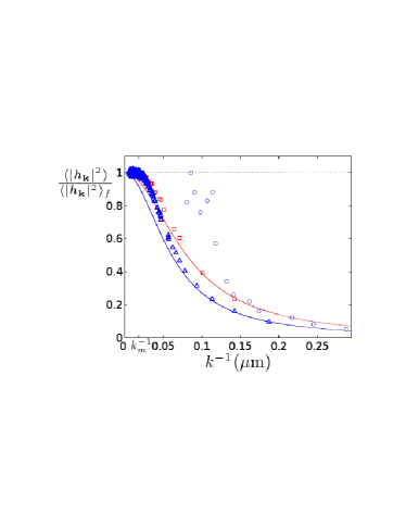
Figure 5: UPPER: Spectrum of fluctuations, $\langle|h_{\mathbf{k}}|^{2}\rangle$, (normalized by $\langle|h_{\mathbf{k}}|^{2}\rangle_{f}$) versus inverse wavenumber for the our RBC membrane model assuming a perfectly intact cytoskeletal network. The squares and triangles indicate simulation results for square and hexagonal meshworks respectively. The error bars are approximately the same size as the symbols. The solid lines are theoretical results using Eq. (29) for $\sigma_{eff}$ and $\kappa_{eff}=\kappa$ in Eq. 19. The wavevector $k_{m}=2\pi/A$ is indicated on the horizontal axis to show where crossover from free membrane to long-wavelength behavior might be expected to occur. The circles are experimental results taken from Ref. Zilker et al. (1987). LOWER: The approach of $\sigma$ to its limiting long-wavelength value is displayed. In this case, each point in the spectrum on the left was individually fit to eq. 19 by adjusting $\sigma_{eff}$ (assuming $\kappa_{eff}=\kappa$). The resulting $\sigma_{eff}$ as a function of $k^{-1}$ are shown. At the longest wavelengths simulated, the inferred tensions converge to the predicted values.

Our simulation results are shown in Fig. 5. In the long wavelength limit, the results are well fit by eq. 19, assuming $\kappa_{eff}=\kappa$ and using

$$\sigma_{s}=\mu,\ \ \sigma_{h}=\sqrt{3}\mu.$$ (29)

for the effective tension in the square and hexagonal symmetry simulations, respectively. These tension values are not fit constants, but rather may be inferred from the cytoskeletal contribution to eq. LABEL:eq:H. Surface tension is an energy per unit area, so we may calculate its value as the ratio of entropic spring (cytoskeleton) energy per corral to the area per corral. In the square geometry, there are effectively two springs per corral (each spring is shared by two adjacent corrals) and using an idealized zero temperature geometry, a single corral has area $A^{2}$ and total spring energy of $2\times\frac{\mu}{2}A^{2}$. The reported value for $\sigma_{s}$ follows immediately. A similar calculation leads to the somewhat larger value of $\sigma_{h}$ in the hexagonal geometry, reflecting the higher density of springs in this case. The numerical value of $\sigma_{h}$ so calculated is $1.3\times 10^{3}$ k_BT $\mu$m${}^{-2}=5.3\times 10^{-6}$ J m^-2, which is close to a theoretical fit Fournier et al. (2004) of the experimental result Zilker et al. (1987) (see Fig. 5).

The fluctuation spectra in fig. 5 indicate that free membrane predictions hold reasonably well out to wavelengths of approximately $A$ ($k^{-1}=A/(2\pi)\sim 0.02\mu\mathrm{m}$), with good convergence to long-wavelength behavior established by $5A$ ($k^{-1}\sim 0.1\mu\mathrm{m}$). The intermediate regime between wavelengths of $A$ to $5A$ encompasses the crossover between the two limiting cases. While this fact is unfortunate in light of the experimental data for the RBC Zilker et al. (1987), which displays a crossover at longer wavelengths, the simulation predictions are unambiguous. The experimental data remains a mystery, but we do note that it may be accounted for by adoption of an ad hoc harmonic confining potential Gov et al. (2003).

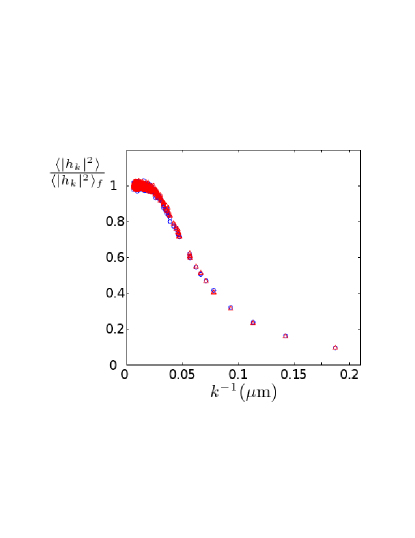
Figure 6: Simulation results of $\langle|h_{\mathbf{k}}|^{2}\rangle$ for a hexagonal lattice. The circles are the data for the case of immobile nodes placed on a perfect lattice. While the triangles are the data for the case of mobile nodes (identical data to fig. 5). Mobility of the cytoskeleton attachment points does not significantly alter the simulation results.

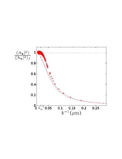
Figure 7: Comparison of different theories for a hexagonal lattice. The circles are the simulation results. The dashed line is the prediction introduced in fig. 5. The solid line is the DF model prediction. At intermediate wavelengths DF does a slightly superior job in fitting the simulations. Both approximations fail at small wavelengths and converge to the same behavior at long wavelengths.

One of the motivations for this work was to test the performance of the analytical theory developed in DF. In particular, we anticipated that the mobility of cytoskeletal anchors would lead to some quantitative deviations from the DF theory at short wavelengths. In fact, the mobility of anchor points leads to insignificant changes in the fluctuation spectrum for physical parameters relevant to the RBC (see fig. 6). We also note that the detailed analysis of DF does slightly better in reproducing the simulated spectrum than does the adoption of surface tensions implied by eq. 29 (see fig. 7). At intermediate wavelengths, the small deviations of $\kappa_{eff}$ away from $\kappa$ predicted by DF do improve the fit as compared to our naive arguments, however the effect is very slight in comparison to the leading order effect of introducing a finite surface tension. As a final point, we note that the anisotropic nature of the square network over all wavelengths leads to some variance in fluctuations for a given magnitude of $k$ depending on the direction taken. In principle, the hexagonal network should not suffer from this effect Boal (2002), however the underlying square lattice taken for our simulations does introduce some anisotropy to the spectra; these effects are most severe at short wavelengths. The spread of data points plotted in figs. 5 - 7 reflects this directional dependence in the spectra and should not be taken as evidence of statistical noise. As previously mentioned, statistical errors are less than the size of the symbols used in plotting.

V Effective surface tension in the presence of a cytoskeletal meshwork with dynamically evolving connectivity

We now generalize the results of the previous section to include RBC membranes with randomly (and dynamically changing) broken cytoskeletal meshworks. As outlined in section II, we assume the dynamics of spectrin association and disassociation are governed by simple rate processes. The rate constants for connecting a broken cytoskeletal filament, $k_{c}$, and breaking an intact filament, $k_{d}$, are assumed independent of the distance between filament end points on the bilayer surface and independent of all other connections within the network. This immediately leads to the conclusion that the probability for a filament to be intact at a given time is $p=k_{c}/(k_{c}+k_{d})$. Equivalently, $p$ is the average percentage of intact filaments in the cytoskeletal network. For the moment, we simply take this picture as a hypothetical model for non-equilibrium dynamics in the RBC membrane. A discussion regarding the connection between this model and experiment will be provided in sec. VI.

Our analysis in this section centers around the calculation of $\sigma(p)$, the effective tension of the composite membrane as inferred from long wavelength fluctuations. As indicated by the notation, this tension depends on the degree of connectivity within the network. Not apparent in the notation is the fact that this tension also depends upon the magnitude of the rates $k_{d}$ and $k_{c}$ (and not just the ratio of them in $p$) due to the non-equilibrium nature of the dynamics. Extraction of $\sigma(p)$ follows the same general prescription as in the previous section; the fluctuation spectrum is collected and compared to the empirical result of eq. 19. At the longest wavelengths modeled in the simulations, it is found that eq. 19 does a good job of reproducing the simulation data. Obvious theoretical estimates for $\sigma_{eff}=\sigma(p)$ are only available in the limiting cases of very fast spectrin (re)association kinetics and very slow kinetics. In general, the effective tension as a function of $p$ (and kinetic rates) must be extracted from simulation.

In the limit that spectrin (re)association rates are much faster than all other time scales in the problem, each cyotoskletal link in the network behaves as an intact link with a diminished spring constant. The numerical value for this weakened spring constant is simply the time average of the spring as it flips between the two possible values of $\mu$ and zero. This picture immediately leads to

$$\sigma_{s}(p)=p\mu,\ \ \sigma_{h}(p)=\sqrt{3}p\mu.\ \ \ \ \ \ (\mathrm{fast\ \ spectrin\ \ kinetics})$$ (30)

Similar arguments have been invoked previously to suggest a possible ATP dependence in the shear modulus of the RBC membrane Gov and Safran (2005). Such an ATP concentration dependence may provide an explanation for RBC shape changes as a function of ATP concentration Gov and Safran (2005).

In the opposite regime, when network connectivity kinetics are far slower than any other timescale in the system, the membrane may be regarded as evolving thermally under the influence of quenched network disorder. The behavior of the system in the quenched disorder limit is analogous to the 2D percolation problem Kirkpatrick (1973). As such, it is expected that the effective tension within the system must vanish at some finite critical $p=p_{c}$. For values of $p$ less than $p_{c}$, no global connectivity within the network exists and, consequently, there is no restoring force possible in response to area dilations of the membrane surface. The 2D connectivity percolation limit is known to occur at $p_{c}=2/z$, where $z$ is the bond valence for each node (i.e. $z=4$ with $p_{c}=1/2$ for the square network and $z=6$ with $p_{c}=1/3$ for the triangular network). Furthermore, within the approximation of the mean field theory, it is expected that the decrease in $\sigma$ as $p$ drops from one to $p_{c}$ is linear. That is

$$\sigma_{s}(p)=2\mu(p-1/2),\ \ \sigma_{h}(p)=\frac{3\sqrt{3}}{2}\mu(p-1/3)$$

$$\ \ \ \ \ \ (\mathrm{slow\ \ spectrin\ \ kinetics})$$ (31)

for all $p>p_{c}$ and $\sigma=0$ for $p<p_{c}$. A brief justification for the percolation theory results quoted above may be found in the Appendix.

The discussion of “fast” and “slow” kinetics in the previous paragraph was intentionally left ambiguous, without specification of what time scales these quantities were to be compared with. It seems prudent to avoid a detailed discussion of this issue, due to the many different dynamic scales in this particular problem, however a crude discussion is appropriate. Given our focus on long wavelength elastic properties, the most obvious timescale for comparison is the membrane relaxation time for the longest wavelength under observation. For equilibrium membranes at tension $\sigma$ and bending rigidity $\kappa$, it is well known Brochard and Lennon (1975); Granek (1997) that relaxation of $h_{\mathbf{k}}$ is exponential with a characteristic time

$$\tau_{m}(k)=\frac{4\eta}{\kappa k^{3}+\sigma k}.$$ (32)

This result follows immediately from eq. 11. Considering only the longest wavelength modes in our simulations ($k=2\pi/L_{max}$ with $L_{max}=L$ for the square and $L_{max}=L_{y}$ for the hexagonal simulations) and allowing for tensions between zero and the fully connected network values, we find that $\tau_{m}$ falls in the range of $9\times 10^{-4}\mathrm{s}$ - $8\times 10^{-3}\mathrm{s}$. While these values are only required to hold for homogeneous equilibrium membranes, they were verified to hold reasonably well for the non-equilibrium membranes studied here when $\sigma(p)$ (determined from the fluctuation spectrum) is naively used in eq. 32. The relaxation rate associated with the two-state spectrin dynamics is $(k_{c}+k_{d})$, which provides a time scale $\tau_{cd}=1/(k_{c}+k_{d})$. The fast kinetics limit discussed above would be expected to apply for $\tau_{m}\gg\tau_{cd}$ and the slow kinetics limit would apply for $\tau_{m}\ll\tau_{cd}$.

FSBD simulations were run including KMC breaking and reforming events in the spectrin meshwork (as detailed in sec. III). Although no equilibrium can be reached in these simulations due to the intrinsically non-equilibrium nature of the simulation, the systems do converge to a steady state regime. $\langle|h_{\mathbf{k}}|^{2}\rangle$ as a function of $k$ were collected, at steady-state, for both the square and hexagonal systems described in the previous section. Three different sets of simulations were run in each geometry corresponding to different spectrin kinetic regimes. Specifically, $k_{d}$ was chosen to assume the values $10^{4}$ s^-1, $200$ s^-1, and $10$ s^-1. A variety of different connectivity percentages were simulated, spanning $0<p<1$. Given values for $k_{d}$ and $p$, $k_{c}=k_{d}p/(1-p)$ follows immediately allowing for complete specification of the model. The three choices for $k_{d}$ roughly correspond to the regimes $\tau_{cd}\ll\tau_{m}$, $\tau_{cd}\sim\tau_{m}$, and $\tau_{cd}\gg\tau_{m}$ respectively.

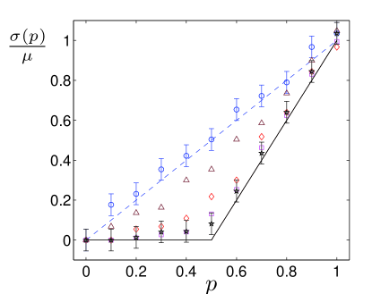
Figure 8: $\sigma(p)/\sigma(p=1)$ versus $p$ is plotted for a square meshwork. The circles, triangles, and diamonds are FSBD/KMC results for $k_{d}=10^{4}s^{-1}$ ($\tau_{cd}\ll\tau_{m}$), $k_{d}=200s^{-1}$ ($\tau_{cd}\sim\tau_{m}$) and $k_{d}=10s^{-1}$ ($\tau_{cd}\gg\tau_{m}$) respectively. The squares and the stars are FMC results ($k_{d}=k_{c}=0$). All simulations use box sizes identical to those introduced in the previous section, except for the stars. Stars represent FMC simulations on systems that are twice as large in both linear dimensions. For clarity, only error bars for the circles and the stars are shown, but all simulations have similar errors. The dashed line is the prediction of Eq. (30). The solid line is the prediction of Eq. (31).

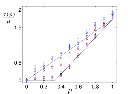
Figure 9: $\sigma(p)/\sigma(p=1)$ versus $p$ is plotted for a hexagonal meshwork. All symbols and lines have the same meaning as in Fig. 8, only the meshwork connectivity has been changed. (The obvious discrepancy between simulation and theory at $p=1$ is due to the rectangular geometry of our simulation box. It is impossible to perfectly fit a portion of a hexagonal network within a rectangle, so the theoretical results that assume perfect hexagonal symmetry are only approximately valid in this case.)

Figures 8 and 9 display our simulation results, plotted in the form of effective surface tensions as a function of network connectivity. The tensions are calculated as in the lower panel of Fig. 5 using the largest wavelengths available in the simulations. In addition to the FSBD/KMC simulations, FMC results are plotted for the quenched disorder case corresponding to $(k_{c}+k_{d})=0$. In these simulations, an ensemble of random network connectivities consistent with the prescribed $p$ values were run without allowing the network connectivity to evolve. The results for $\langle|h_{\mathbf{k}}|^{2}\rangle$ were averaged over the ensemble to obtain $\sigma(p)$. FMC was used in these cases for numerical efficiency and is valid since the evolution under conditions of static network connectivity is purely thermal. The speed of the FMC algorithm allowed a set of simulations to be run for larger membrane sizes in order to clarify the role of finite size effects.

The figures clearly display both expected regimes. Fast network reorganization yields results in good agreement with eq. 30, whereas slow reorganization yields results consistent with eq. 31. Intermediate kinetic regimes interpolate between these two limiting cases. Finite size effects appear not to play any role, except perhaps for the case of $p$ values very close to $p_{c}$ in the quenched disorder case, which is to be expected due to the percolation phase transition at this point. At values of intermediate membrane connectivity, it is possible for the systems to display a range of effective surface tension values, depending upon the relative timescales for spectrin kinetics as compared to membrane relaxation. The implications of this fact will be discussed further in the next section.

VI Connection to experiments

Evidence that RBC membrane shapes and shape fluctuations depend upon non-thermal energy expenditure comes from two different experimental sources. Measurement of cell shape Sheetz and Singer (1977) and shape fluctuations Levin and Korenstein (1991); Tuvia et al. (1998) under a variety of MgATP concentrations suggest this fact directly. Increases in MgATP concentration lead to enhanced membrane surface fluctuations. Less directly, it has been shown that RBC membrane fluctuation amplitudes in the presence of MgATP depend upon the viscosity of the surrounding solvent Tuvia et al. (1997). Thermal properties of a physical system should not be influenced by transport coefficients, such as the viscosity, but should depend only upon system energetics via the partition function.

Biochemically, it is clear that the presence of MgATP leads to the phosphorylation of spectrin Birchmeier and Singer (1977), which has been implicated in the observed shape changes and fluctuation amplitudes in RBC membranes under varying MgATP concentrations Sheetz and Singer (1977). Whether or not this phosphorylation event (and/or similar events in other molecular components of the network) coincides with breaking of spectrin filaments is less clear, however the hypothesis that this is in fact the case Gov and Safran (2005) is compelling and served as one of the major motivations for this study. In what follows, we assume that phosphorylation of spectrin induces individual filaments to dissociate from the network. We stress that this model is hypothetical and, indeed, that some studies refute the correlation between spectrin phosphorylation and RBC shape/elastic properties Patel and Fairbanks (1981); Bordin et al. (1995).

In a naive model for spectrin phosphorylation, we assume the following kinetic equations for spectrin dissociation and association with the network as a whole.

$$\mathrm{S_{a}}+\mathrm{ATP} \stackrel{{\scriptstyle k_{d}}}{{\rightarrow}} \mathrm{S_{d}}+\mathrm{ADP}$$ (33)

$$S_{d}+\mathrm{H_{2}O} \stackrel{{\scriptstyle k_{c}}}{{\rightarrow}} \mathrm{S_{a}}+\mathrm{HPO_{4}^{2-}}.$$

In the above, $\mathrm{S_{a}}$ and $\mathrm{S_{d}}$ stand for the associated and dissociated forms of spectrin, respectively, and it is assumed that the reactions proceed via catalysis by kinases and phosphatases. We assume ATP concentration is held fixed, either by endogenous biochemistry within the RBC in vivo or by experimental control in vitro. Using our previously introduced notation, we write $[\mathrm{S_{a}}]=Cp$ and $[\mathrm{S_{d}}]=C(1-p)$, where $C$ is the total concentration of spectrin on the cell surface. The steady state condition is formulated as $dp/dt=0$, which, in conjunction with kinetic eqs. 33, leads to

$$p=\frac{n_{c}}{n_{c}+2n}.$$ (34)

Here, both kinetic constants have been wrapped up into the single constant $n_{c}$. $n$ is the concentration of ATP in solution. $n_{c}$ has been defined such that the condition $n=n_{c}$ implies $p=p_{c}=1/3$ (in this section we assume the hexagonal network due to its direct connection to RBC systems) , i.e. $n=n_{c}$ specifies the concentration of ATP necessary to reach the percolation phase transition in systems with quenched disorder. While this model neglects the observed dependence of spectrin dephosphorylation on $n$ Birchmeier and Singer (1977), it has the advantage of simplicity in the absence of quantitative kinetic data and follows the line of reasoning previously introduced Gov and Safran (2005), allowing for comparison to earlier work. Eq. 34 predicts the connectivity of the network as a function of ATP concentration and allows for comparison between the modeling of the previous section and experimental data.

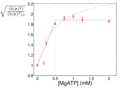
Figure 10: Real space RBC height fluctuations, $\sqrt{\langle h(\mathbf{r})^{2}\rangle}$, as a function of ATP concentration (normalized by the zero ATP values, $\sqrt{\langle h(\mathbf{r})^{2}\rangle}_{0}$). The circles with error bars are the experimental data Tuvia et al. (1998). The solid line is a theoretical fit assuming $\sigma_{h}$ in Eq. (31), corresponding to the case of $\tau_{m}\ll\tau_{cd}$ (slow spectrin kinetics). The dashed line is a theoretical fit assuming $\sigma_{h}$ in Eq. (30), corresponding to the case of $\tau_{cd}\ll\tau_{m}$ (fast spectrin kinetics).

Experimental data for RBC fluctuations as a function of ATP concentration is available only in terms of real space height amplitudes, $h(\mathbf{r})$ Tuvia et al. (1998) (see fig. 10). Following Eqs. (12) and (19) (and for simplicity assuming $L_{x}=L_{y}=L$),

$$\langle h(\mathbf{r})^{2}\rangle=\sum_{\mathbf{k}}\frac{k_{B}T}{L^{2}(\kappa k^{4}+\sigma k^{2})},$$ (35)

where the interval between adjacent $k_{x}$ or $k_{y}$ is $2\pi/L$. In the limit of large $L$, the sum $\sum_{\mathbf{k}}$ can be approximated by the integral $L^{2}/(2\pi)^{2}\int d\mathbf{k}$, and we have

$$\langle h(\mathbf{r})^{2}\rangle=\frac{k_{B}T}{4\pi\sigma}\ln(1+\frac{\sigma L^{2}}{\pi^{2}\kappa}).$$ (36)

The limiting expressions and simulations of the preceding section provide a route toward estimation of $\sigma(p)$ under various rates of spectrin association/dissociation. Eq. 34 enables us to translate these results into tensions as a function of ATP concentration. The resulting tensions may be used in eq. 36 to calculate the real space membrane fluctuation amplitudes as a function of ATP concentration. RBC’s have a diameter of 7 microns and we use $L=7\mathrm{\mu m}$ Lodish et al. (1995) in our comparison to experiment. It is also important to note that experimental observations of RBC fluctuations were carried out on cells that were allowed to “firmly adhere to [a] glass substratum” Tuvia et al. (1998) under the influence of their natural (presumably of electrostatic origin) affinity for such surfaces. The adhesion of the bilayer to an underlying supporting matrix will be assumed to contribute a bare surface tension, $\sigma_{bare}$ to the membrane of the RBC Brochard et al. (1976); Lin et al. (2006). That is, we assume $\sigma=\sigma_{bare}+\sigma(p)$.

We take $n_{c}$ and $\sigma_{bare}$ as two fitting parameters to reproduce the experimental data. The resulting fits, assuming the two extreme cases of fast spectrin kinetics (eq. 30 assumed) and slow spectrin kinetics (eq. 31 assumed) are displayed in fig. 10. The values adopted by the fitting parameters in these two cases are $\sigma_{bare}=0.2\mu=150\mathrm{k_{B}T/\mu m^{2}}$ (both cases), and $n_{c}=0.22$ mM for the fast kinetics case and $n_{c}=0.5$ mM for the slow kinetics case. It turns out that the limiting case of slow spectrin kinetics provides the most satisfactory fit of the data, not only in comparison to the fast kinetics case, but also with respect to intermediate kinetic regimes; the sharp onset of tensionless fluctuations at $n_{c}$ naturally leads to the observed plateau in the experimental data.

The slowest possible time-scale associated with RBC membrane fluctuations in our model ($\tau_{m}$) is on the order of a couple of seconds. This assumes a tension-free membrane and $L=7\mu$m. Our data analysis suggests that spectrin breaking/reformation dynamics are substantially slower than this, since the quenched-disorder (percolation theory) results provide the best fit to the experimental data. This finding would appear to be consistent with the experimental observation Birchmeier and Singer (1977) that establishment of steady-state levels of spectrin phosphorylation occurs on the time scale of minutes to tens of minutes with changes in MgATP concentration. Previous theoretical work exploring the consequences of spectrin dissociation on membrane fluctuations Gov and Safran (2005) has assumed the time-scale for spectrin kinetics to be on the order of milliseconds. Within the context of the present model, rates this fast seem unlikely.

Experimentally, it is observed that RBC fluctuation amplitudes depend not only upon MgATP concentration, but also upon the viscosity of the solvent surrounding the membrane Tuvia et al. (1997); increasing viscosity above that of aqueous buffer solution leads to decreases in observed fluctuations. Membrane fluctuations at thermal equilibrium should yield identical statistics regardless of solvent viscosity (although the dynamics will certainly differ), so these experiments provide additional proof of the non-thermal character of RBC fluctuations.

Within the present model, Eq. (32) clearly displays the linear relationship between inverse viscosity and the relaxation timescales for individual membrane modes. In the preceding section, it was argued that the ratio between membrane relaxation rates and spectrin kinetic rates determines the magnitude of effective tension that must be used if one desires to fit membrane fluctuations to the functional form of eq. 19. At a given connectivity, $p$, fluctuation amplitudes decrease ($\sigma_{eff}$ increases) as the spectrin kinetic cycle increases in speed. Alternatively, since it is the ratio of kinetics to membrane relaxation that is relevant, we expect fluctuation amplitudes to decrease as viscosity is raised assuming all other system parameters are held fixed. Qualitatively, this trend is in agreement with the experimental results.

To obtain quantitative comparison with the variable viscosity data it is necessary to evaluate $\langle h(\mathbf{r})^{2}\rangle$ explicitly from direct simulation, without assuming a single effective tension as in eq. 35. Within our model, fluctuation amplitudes are affected by viscosity changes only by shifting the timescale for membrane dynamics relative to spectrin kinetics. A relative shift in timescale (at constant $p$) corresponds to a vertical motion between the limiting regimes plotted in fig. 9. In order for viscosity changes to yield any effect, the timescales for spectrin kinetics and membrane relaxation must be comparable. (e.g. if spectrin dissociation takes an hour, increasing viscosity by a factor of 10 will not remove you from the limiting “slow kinetics regime”. Similarly, if dissociation took a nanosecond, no reasonable viscosity change could promote the system out of the “fast kinetics regime”.) And, if these timescales are comparable, differences in the individual relaxation rates at each wavelength will lead to different effective tensions as a function of wavelength. In practice, it is not feasible to run simulations for a full $7\mu m\times 7\mu m$ patch with sufficient sampling to obtain reliable results. It is possible to run a $1\mu m\times 7\mu m$ patch. The effective tensions as a function of wavevector were extracted from this rectangular geometry and were used in a generalized version of eq. 35 with $\sigma\rightarrow\sigma(k)$ to obtain $\langle h(\mathbf{r})^{2}\rangle$ for the full $7\mu m\times 7\mu m$ system.

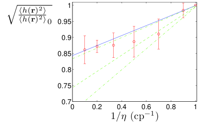
Figure 11: Normalized height fluctuations, $\sqrt{\langle h(\mathbf{r})^{2}\rangle}$, as a function of inverse viscosity of the solvent. The circles with error bars are the simulation results assuming $L=7$ $\mu$m, $\sigma_{bare}=150\mathrm{k_{B}T/\mu m^{2}}$, $n_{c}=0.5$ mM, $n=1.2$ mM and $\tau_{cd}=5\times 10^{5}\mu$s. The solid line is a fit to our simulation data. The dashed line and the two dashdotted lines are the experimental fitting line and the range of experimental errors taken from Fig. 2 of Ref. Tuvia et al. (1997).

To simultaneously find agreement with the ATP concentration data (fig. 10) and the variable viscosity data it is necessary to assume spectrin rates that are slow relative to membrane relaxation when the solvent is pure buffer solution (as in the conditions of ref. Tuvia et al. (1998) and fig. 10), but are poised to move out of this limiting regime with small viscosity increases. By trial and error, it was found that $\tau_{cd}=5\times 10^{5}\mu$s for $n=1.2$ mM (the ATP concentration conditions of ref. Tuvia et al. (1997)) satisfies this condition and yields the best fit to both data sets. Other model parameters were taken identical to the “slow spectrin kinetics” fit to the data of fig. 10. In particular, $L=7\mathrm{\mu m}$, $n_{c}=0.5$ mM and $\sigma_{bare}=150\mathrm{k_{B}T/\mu m^{2}}$. In fig. 11 we plot real space membrane fluctuations as a function of $\eta^{-1}$ for viscosity values spanning an order of magnitude. We observe a reduction in fluctuation amplitudes of about 20% over the entire range of viscosities studied, which falls just outside the errors of the experimental data Tuvia et al. (1997). It is important to stress that figs. 10 and 11 simultaneously fit two very different experiments to a single set of physical parameters. Our results agree with both experiments quite well.

VII Discussion

From a mathematical standpoint, the results of the preceding section could be viewed as a success; we fit the available experimental data with our theoretical model. However, the physical implications of the derived fit parameters are troubling. Most worrisome is the critical concentration of ATP for onset of the percolation limit, $n_{c}=0.5$ mM. This implies that at physiological conditions ($n\sim 2$ mM), the spectrin network is 89% dissociated. A similar degree of dissociation (83 %) is predicted for the $n=1.2$ mM conditions of the variable viscosity experiments described above. As presented, it is clear that our model should not be taken seriously in the limit of slow spectrin kinetics and $n\geq n_{c}$, since we do not allow the connectivity of the network to evolve away from its starting point (i.e. a given spectrin tetramer is assumed to always link the same two vertices or be disassociated). In a severely compromised network, how could a given filament ever be expected to find its assigned association point following a dissociation event?

As mentioned previously, there does not appear to be definitive experimental data relating ATP consumption to spectrin network dissociation. Rather, this is a plausible hypothesis advocated in reference Gov and Safran (2005), based upon the limited biochemical data that is available for the various constituents of the RBC cytoskeleton. We can not reconcile this picture with the simulations carried out in this work, primarily for the reason outlined in the previous paragraph. It is possible that ATP consumption could lead to a significant change in the elastic properties of individual spectrin filaments without completely dissociating the filament from the network. In such a picture, the two forms of spectrin introduced above, $S_{d}$ and $S_{a}$, would correspond to filaments with weak and strong effective spring constants, respectively (or different natural lengths, etc.). In this context, the analysis we present is sensible since network connectivity is always maintained, but the elastic properties of individual links are changing. The percolation limit in this picture corresponds to the point at which it is impossible to follow a path across the spectrin network without stepping on at least one weak $S_{d}$ link. Although such a picture is completely hypothetical, we note that it is theoretically possible to alter the effective elastic properties of spectrin filaments while maintaining lateral integrity of the network Gov (2007); Zhu and Asaro (2008).

The underlying physical picture pursued in this work was motivated by and is similar in spirit to the work of Safran and Gov Gov and Safran (2005) (i.e. a dynamically breaking and reforming spectrin network). However, the simulation model implemented to study this system is more similar to the work of Dubus and Fournier Dubus and Fournier (2006) (with the additional possibility of dynamically breaking bonds). We have interpreted our simulation results within the context of a simple percolation theory. While this picture shares some similarity with the analysis of ref. Gov and Safran (2005) in the context of global effects associated with variable ATP concentration, we find differences between the present model and ref. Gov and Safran (2005) in the description of local fluctuation dynamics. For example, we find no evidence in our simulations for localized forces of the sort discussed in ref. Gov and Safran (2005). Instead, the increased amplitudes of fluctuation at high ATP concentration are attributable to global properties of the spectrin network within our model. We also find that the rates associated with spectrin kinetics must be orders of magnitude slower than assumed in ref. Gov and Safran (2005) in order to reconcile our simulation model with the experiments of refs. Tuvia et al. (1998, 1997). However, it should be pointed out that the particular rates assumed in ref. Gov and Safran (2005) were only rough estimates and are not essential to the qualitative predictions of that work nir .

The starting point for all of our simulations, eq. LABEL:eq:H, assumes a central-force network for the cytoskeletal matrix and a phantom entropic spring description for the spectrin filaments. In addition, we do not allow for the possible formation of 5-fold or 7-fold defects Seung and Nelson (1988); Gov and Safran (2005) in our network. Inclusion of direct interactions between spectrin and the bilayer surface, generalizing the description of the network to deviate from the central-force picture, and/or allowing for defects in network connectivity could all potentially alter the quantitative findings of this work. The present simulation model was adopted for ease of numerical implementation and to facilitate comparison to the existing work of Dubus and Fournier Dubus and Fournier (2006). This study provides a detailed analysis of the behavior of a specific model for a composite membrane system (lipid bilayer plus actively labile cytoskeletal network). This model is motivated by our (incomplete) picture for the structure and kinetics of the RBC membrane surface and may prove useful in the development of more refined models in the future. In particular, it should be noted that more refined descriptions of the spectrin network have been developed that allow for interactions between the bilayer surface and the filaments and a more complete description of polymer elasticity beyond the simple Gaussian-chain model Boal (1994); Li et al. (2007); Zhu et al. (2007). Future modeling, incorporating some of these approaches for the behavior of the cytoskeleton, would be highly desirable and is currently under investigation.

We note in closing that a very recent study by Evans et. al. Evans et al. (2008) directly contradicts the experimental results in refs. Tuvia et al. (1998, 1997). This recent series of experiments finds no correlation between ATP concentration and RBC membrane fluctuations. Given the severe disagreement between experimental results on the RBC system, one has almost complete freedom in interpretation of our simulation results. The picture outlined above suggests that we can obtain quite good agreement between simulation and experiments that do measure ATP dependence of the RBC fluctuations. Within this picture, it seems necessary to assume that our “broken” spectrin links actually correspond to intact links with diminished spring constant and/or a non-zero natural length. Another, equally valid, interpretation of our results is that it is impossible to reconcile an actively breaking cytoskeletal meshwork picture with available experimental data due to the high degree of network dissociation predicted under physiological conditions within such a picture. Given the uncertain experimental landscape, it seems impossible to make a definitive statement in favor of either viewpoint.

Appendix

The calculation of an effective tension in the limit of quenched disorder within the spectrin network is closely related to the 2D bond percolation problem Stauffer and Aharony (1994). A mean field treatment for the percolation problem was first developed in the context of electric conductivity Kirkpatrick (1973) and was later extended to calculate the elastic moduli of networks of Hookean springs with finite Feng et al. (1985); Feng and Sen (1984) and zero natural lengths Tang and Thorpe (1987, 1988). The below discussion summarizes the arguments of Ref. Feng et al. (1985) for the readers’ convenience.

Let us consider a randomly connected meshwork with only a fraction ($p$) of the links intact. Each intact link is a spring with spring constant $\mu$ and a natural extension of zero. In the spirit of mean field theory, we assume that the global elastic properties of this imperfect meshwork are well approximated by a complete meshwork comprised of springs with spring constant $\mu_{m}$ at every link (see Fig. 12) even though individual links will be either completely intact or fully broken. Our problem is to determine an expression for $\mu_{m}$. For this purpose, let us consider an arbitrary link $AB$ in the meshwork. The real spring constant, $\mu_{AB}$, associated with this link is either $\mu$ if the link is connected, or 0 if it is not. If we apply a force $f_{m}$ across this link (see Fig. 12), the extension $x_{AB}$ is given by

$$x_{AB}=\frac{f_{m}}{\mu_{AB}+\mu_{eff}},$$ (37)

where $\mu_{eff}$ is an effective spring constant reflecting the contribution of all network components except the link $AB$. It can be shown that Feng et al. (1985)

$$\mu_{eff}=(z/2-1)\mu_{m},$$ (38)

where $z$ is the connectivity of the meshwork, for example, $z=4$ for the square meshwork and $z=6$ for the hexagonal meshwork considered in this work.

On the other hand, if we assume the mean spring constant $\mu_{m}$ for link $AB$, we predict a mean extension,

$$x_{m}=\frac{f_{m}}{\mu_{m}+\mu_{eff}}.$$ (39)

To achieve consistency within the mean field approximation, we must have

$$\langle x_{AB}\rangle = x_{m}$$ (40)

$$\frac{pf_{m}}{\mu+\mu_{eff}}+\frac{(1-p)f_{m}}{\mu_{eff}} = \frac{f_{m}}{\mu_{m}+\mu_{eff}}$$

where the second equality is simply a more explicit version of the first. This equation is readily solved to yield

$$\mu_{m}=\frac{p-p_{c}}{1-p_{c}}\mu,$$ (41)

where

$$p_{c}=2/z.$$ (42)

To calculate $\sigma(p)$, we simply replace $\mu$ in eq. 29 by $\mu_{m}$ from eq. 41, since the latter is now the average spring constant of the equivalent complete meshwork. Taking $z=4$ and $z=6$ for the square and hexagonal meshwork respectively, we arrive at eq. 31.

One should note that eqs. 31 and 42 are only results of a mean field approximation. In the vicinity of $p_{c}$, it is well known that the correlation effects are strong and that mean field theory breaks down. However, the mean field results are adequate to describe the behavior of $\sigma$ outside the immediate vicinity of $p_{c}$ as evidenced by figs. 8 and 9, which is sufficient for the purposes of this work.

Table 1: Physical parameters in simulations

Parameter	Description	Value	Reference
$\kappa$	bending modulus	4.8 kBT	Brochard and Lennon (1975)
$\eta$	cytoplasm viscosity	1.5 kBT s $\mu$m-3	Brochard and Lennon (1975)
$D$	diffusion constant of nodes	0.53 $\mu$m2 s-1	Tomishige et al. (1998)
$A$	the average distance between two nearest nodes (see Fig. 4)	0.112 $\mu$m	Boal (2002)
$\ell_{c}$	contour length of the spectrin tetramer	0.2 $\mu$m	Boal (2002)
$\ell_{k}$	Kuhn length of the spectrin tetramer	0.02 $\mu$m	Boal (2002)
$\mu$	spring constant of the spectrin tetramer	750 kBT $\mu$m-2

Figure 1: A schematic rendering of the RBC membrane. (a): Top View: Looking down on the cell with the lipid bilayer invisible for clarity. The nodes of the cytoskeletal network are protein complexes embedded in the lipid bilayer. The links are spectrin tetramers, with approximate lateral end-to-end distance of $100nm$ between the nodes. (b): Side View: The protein anchors are confined to the lipid bilayer, but may diffuse laterally. The coils underneath the bilayer are spectrin tetramers. The contour length of the tetramers is approximately $200nm$, so there is considerable extra length coiled up below the membrane surface. (c): One end of a link is disconnected from the node, possibly with the help of ATP.

Figure 3: A schematic illustration of a randomly broken spectrin meshwork. The solid lines are connected links while the dotted lines represent disconnected ones. The percentage of intact links (equivalently, the probability for any single link to be intact) will be denoted “$p$”. All lines together (solid and dotted) correspond to a complete hexagonal meshwork. (a): Above the percolation threshold, $p>p_{c}$, the connected links have global connectivity, i.e., they form a cluster extending across the entire cell. The corresponding effective surface tension will always be finite. (b): Below the percolation threshold, $p<p_{c}$, there is no global connectivity in the meshwork, i.e. connected links form finite islands of connectivity that do not span the cell. The corresponding effective surface tension becomes zero if the links are breaking and reforming slowly. (c): Even at instantaneous connectivities below the percolation threshold, there can be a finite surface tension if spectrin breaking/formation kinetics are sufficiently fast. In this limit, each link can be thought of as a spring with a reduced restoring force since out of plane membrane undulations evolve more slowly than the lifetime of the link.

Figure 4: A schematic illustration of the connectivity of the nodes of the meshwork. (a): the hexagonal meshwork. The dotted lines are a guide of eyes for the rectangular sample used. (b): the square meshwork.

Figure 12: (a) A randomly broken network of springs is approximated by a complete meshwork of springs with diminished spring constant $\mu_{m}$. Here we imagine an attempt to extend the link $AB$ using a force of $f_{m}$. (b) The force $f_{m}$ is resisted both directly by link $AB$ and the rest of the meshwork. The latter can be considered as a single spring with effective spring constant $\mu_{eff}$, which acts in parallel with $AB$. (Adapted from ref. Feng et al. (1985))

References

- Alberts et al. (2002) B. Alberts, A. Johnson, J. Lewis, M. Raff, K. Roberts, and P. Walter, Molecular Biology of the Cell (Galland, New York, 2002).
- Safran (2003) S. A. Safran, Statistical Thermodynamics of Surfaces, Interfaces, and Memebranes (Westview Press, Boulder, CO, 2003).
- Gre (1995) Structure and Dynamics of Membranes, edited by R. Lipowsky and E. Sackmann (Elsevier Science, Amsterdam, 1995).
- Liu et al. (1987) S. Liu, L. Derick, and J. Palek, J. Cell. Biol. 104, 527 (1987).
- Brochard and Lennon (1975) F. Brochard and J. F. Lennon, J. Phys. (Paris) 36, 1035 (1975).
- Peterson (1992) M. A. Peterson, Phys. Rev. A 45, 4116 (1992).
- Gov et al. (2003) N. Gov, A. G. Zilman, and S. Safran, Phys. Rev. Lett. 90, 228101 (2003).
- Lim et al. (2002) G. H. W. Lim, M. Wortis, and R. Mukhopadhyay, Proc. Nat. Acad. Sci. USA 99, 16766 (2002).
- Fournier et al. (2004) J.-B. Fournier, D. Lacoste, and E. Raphael, Phys. Rev. Lett. 92, 018102 (2004).
- Rochal and Lorman (2006) S. B. Rochal and V. L. Lorman, Phys. Rev. Lett. 96, 248102 (2006).
- Zilker et al. (1987) A. Zilker, H. Engelhardt, and E. Sackmann, J. Phys. (Fr.) 48, 2139 (1987).
- Discher et al. (1994) D. Discher, N. Mohandas, and E. A. Evans, Science 266, 1032 (1994).
- Heinrich et al. (2001) V. Heinrich, K. Ritchie, N. Mohandas, and E. Evans, Biophys. J. 81, 1452 (2001).
- Engelhardt et al. (1984) H. Engelhardt, H. Gaub, and E. Sackmann, Nature (London) 307, 378 (1984).
- Birchmeier and Singer (1977) W. Birchmeier and S. J. Singer, J. Cell Biol. 73, 647 (1977).
- Bennett (1989) V. Bennett, Biochim. Biophys. Acta 988, 107 (1989).
- Levin and Korenstein (1991) S. Levin and R. Korenstein, Biophys. J. 60, 733 (1991).
- Tuvia et al. (1998) S. Tuvia, S. Levin, A. Bitler, and R. Korenstein, J. Cell Biol. 141, 1551 (1998).
- Gov and Safran (2005) N. Gov and S. A. Safran, Biophys. J. 88, 1859 (2005).
- Tuvia et al. (1997) S. Tuvia, A. Almagor, A. Bitler, S. Levin, R. Korenstein, and S. Yedgar, Proc. Natl. Acad. Sci. USA 94, 5045 (1997).
- Dubus and Fournier (2006) C. Dubus and J.-B. Fournier, Europhys. Lett. 75, 181 (2006).
- Helfrich (1973) W. Helfrich, Z. Naturforsch. pp. 693–703 (1973).
- Nelson and Peliti (1987) D. R. Nelson and L. Peliti, J. Phys. (Paris) 48, 1085 (1987).
- Purcell (1977) E. M. Purcell, American Journal of Physics 45, 3 (1977).
- Granek (1997) R. Granek, J. Phys. II (Paris) 7, 1761 (1997).
- Lin and Brown (2005) L. C.-L. Lin and F. L. H. Brown, Phys. Rev. E 72, 011910 (2005).
- Brown (2008) F. L. H. Brown, Annual Review of Physical Chemistry 59, 685 (2008).
- Doi and Edwards (1986) M. Doi and S. Edwards, The Theory of Polymer Dynamics (Clarendon, Oxford, 1986).
- Reister and Seifert (2005) E. Reister and U. Seifert, Europhys. Lett. 71, 859 (2005).
- Naji and Brown (2007) A. Naji and F. L. H. Brown, J. Chem. Phys. 126, 235103 (2007).
- Boal (2002) D. H. Boal, Mechanics of the cell (Cambridge University Press, Cambridge, UK, 2002).
- Gouliaev and Nagle (1998a) N. Gouliaev and J. F. Nagle, Phys. Rev. E. 58, 881 (1998a).
- Gouliaev and Nagle (1998b) N. Gouliaev and J. F. Nagle, Phys. Rev. Lett 81, 2610 (1998b).
- Lin and Brown (2004a) L. C.-L. Lin and F. L. H. Brown, Biophys. J. 86, 764 (2004a).
- Lin and Brown (2004b) L. C.-L. Lin and F. L. H. Brown, Phys. Rev. Lett. 93, 256001 (2004b).
- Frenkel and Smit (2002) D. Frenkel and B. Smit, Understanding Molecular Simulation (Academic Press, San Diego, 2002), 2nd ed., pp. 525-532.
- Bouzida et al. (1992) D. Bouzida, S. Kumar, and R. H. Swendsen, Phys. Rev. A 45, 8894 (1992).
- Lin and Brown (2006) L. C.-L. Lin and F. L. H. Brown, J. Chem. Theory Comp. 2, 472 (2006).
- Gillespie (1976) D. T. Gillespie, J. Comput. Phys. 22, 403 (1976).
- van Kampen (1992) N. G. van Kampen, Stochastic Processes in Physics and Chemistry (North-Holland, Amsterdam, 1992), pp. 63,83,220-221.
- Press et al. (1994) W. H. Press, S. A. Teukolsky, W. T. Vetterling, and B. P. Flannery, Numerical Recipes in C (Cambridge University Press, Cambridge, 1994).
- Kirkpatrick (1973) S. Kirkpatrick, Rev. of Mod. Phys. 45, 574 (1973), and references therein.
- Sheetz and Singer (1977) M. P. Sheetz and S. J. Singer, J. Cell Biol. 73, 638 (1977).
- Patel and Fairbanks (1981) V. P. Patel and G. Fairbanks, J. Cell. Biol. 88, 430 (1981).
- Bordin et al. (1995) L. Bordin, G. Clari, I. Moro, F. D. Vecchia, and V. Moret, Biochem. Biophys. Res. Comm. 213, 249 (1995).
- Lodish et al. (1995) H. Lodish, D. Baltimore, A. Berk, S. L. Zipursky, P. Matsudaira, and J. Darnell, Molecular Cell Biology (Scientific American Books, New York, 1995), 3rd ed.
- Brochard et al. (1976) F. Brochard, P. G. DeGennes, and P. Pfeuty, J. Phys. (Paris) 37, 1099 (1976).
- Lin et al. (2006) L. C.-L. Lin, J. T. Groves, and F. L. H. Brown, Biophys. J. 91, 3600 (2006).
- Gov (2007) N. S. Gov, New Journal of Physics 9, 429 (2007).
- Zhu and Asaro (2008) Q. Zhu and R. J. Asaro, Biophys. J. 94, 2529 (2008).
- (51) N. S. Gov, personal communication.
- Seung and Nelson (1988) H. S. Seung and D. R. Nelson, Phys. Rev. A 38, 1005 (1988).
- Boal (1994) D. H. Boal, Biophys. J. 67, 521 (1994).
- Li et al. (2007) J. Li, G. Lykotrafitis, M. Dao, and S. Suresh, Proc. Nat. Acad. Sci. USA 104, 4937 (2007).
- Zhu et al. (2007) Q. Zhu, C. Vera, R. J. Asaro, P. Sche, and L. A. Sung, Biophys. J. 93, 386 (2007).
- Evans et al. (2008) J. Evans, W. Gratzer, N. Mohandas, K. Parker, and J. Sleep, Biophys. J (2008), in press.
- Stauffer and Aharony (1994) D. Stauffer and A. Aharony (1994).
- Feng et al. (1985) S. Feng, M. F. Thorpe, and E. Garboczi, Phys. Rev. B 31, 276 (1985).
- Feng and Sen (1984) S. Feng and P. N. Sen, Phys. Rev. Lett. 52, 216 (1984).
- Tang and Thorpe (1987) W. Tang and M. F. Thorpe, Phys. Rev. B 36, 3798 (1987).
- Tang and Thorpe (1988) W. Tang and M. F. Thorpe, Phys. Rev. B 37, 5539 (1988).
- Tomishige et al. (1998) M. Tomishige, Y. Sako, and A. Kusumi, J. Cell Biol. 142, 989 (1998).