3-D Model of Broadband Emission from Supernova Remnants Undergoing Non-linear Diffusive Shock Acceleration

Abstract

We present a 3-dimensional model of supernova remnants (SNRs) where the hydrodynamical evolution of the remnant is modeled consistently with nonlinear diffusive shock acceleration occuring at the outer blast wave. The model includes particle escape and diffusion outside of the forward shock, and particle interactions with arbitrary distributions of external ambient material, such as molecular clouds. We include synchrotron emission and cooling, bremsstrahlung radiation, neutral pion production, inverse-Compton (IC), and Coulomb energy-loss. Boardband spectra have been calculated for typical parameters including dense regions of gas external to a $1000$ year old SNR. In this paper, we describe the details of our model but do not attempt a detailed fit to any specific remnant. We also do not include magnetic field amplification (MFA), even though this effect may be important in some young remnants. In this first presentation of the model we don’t attempt a detailed fit to any specific remnant. Our aim is to develop a flexible platform, which can be generalized to include effects such as MFA, and which can be easily adapted to various SNR environments, including Type Ia SNRs, which explode in a constant density medium, and Type II SNRs, which explode in a pre-supernova wind. When applied to a specific SNR, our model will predict cosmic-ray spectra and multi-wavelength morphology in projected images for instruments with varying spatial and spectral resolutions. We show examples of these spectra and images and emphasize the importance of measurements in the hard X-ray, GeV, and TeV gamma-ray bands for investigating key ingredients in the acceleration mechanism, and for deducing whether or not TeV emission is produced by IC from electrons or pion-decay from protons.

1. Introduction

Supernovae (SNe) are the only known sources capable of providing the energy needed to power the bulk of the galactic cosmic rays (CRs) with energies below the spectral feature called the “knee” around $3\times 10^{15}$ eV (e.g., Drury, 1983). If SNe are the main sources of Galactic CRs, the acceleration mechanism must be efficient so that $\gtrsim 10$% of the total SN explosion energy in our Galaxy ends up in cosmic rays (e.g., Hillas, 2005). Observational evidence that the outer blast wave shock accelerates electrons to ultra-relativistic energies in some young SNRs (e.g., Koyama et al., 1995), and the existence of a well-developed model of particle acceleration at shocks, i.e., diffusive shock acceleration (DSA) (e.g., Drury, 1983; Blandford & Eichler, 1987; Jones & Ellison, 1991) support the above contention.

When confronting observations with theoretical models, however, there remain a number of important ambiguities and uncertainties from both the observational and theoretical perspectives. Resolution of these ambiguities and uncertainties by new telescopes will be essential to claim evidence for the pion-decay feature in the GeV-TeV emission from SNRs. The Gamma-ray Large Area Space Telescope (GLAST), to be launched in 2008, will probe this crucial energy range with unprecedented sensitivity and resolution.

Fundamental questions for CR origin also concern the spectral shape and maximum ion energy a given SNR can produce. Electron energy spectra inferred from young SNRs vary and can be substantially harder than CR electron spectra observed at Earth, even after correction for propagation in the galaxy (e.g., Berezhko & Völk, 2006). The maximum CR ion energy SNRs actually produce will remain uncertain until a firm identification of pion-decay emission is obtained and gamma-ray emission is detected past a few 100 TeV, the maximum possible electron energy in SNRs.

There remain other basic questions concerning the DSA mechanism. For instance, is DSA efficient enough for nonlinear effects, such as shock smoothing and magnetic field amplification, to become important in young SNRs? How does particle injection occur and how does injection and acceleration vary between electrons and protons? While the galactic CR electron-to-proton ratio, $(e/p)_{\mathrm{rel}}$, of $0.01$–$0.0025$ observed at Earth at relativistic energies is often used to constrain the ratio in SNRs, this ratio has not been observed outside of the heliosphere. The $(e/p)_{\mathrm{rel}}$ ratio is crucial in deciding whether the $\gamma$-ray emission from different SNRs, or observed in different parts of an individual SNR, is of hadronic or leptonic origin.

The recent discovery of spatially thin, hard X-ray filaments in some young SNRs (e.g., Bamba et al., 2003; Uchiyama et al., 2007) supports previous suggestions (e.g., Cowsik & Sarkar, 1980; Bell & Lucek, 2001; Reynolds & Ellison, 1992) that the particle acceleration process can amplify the ambient magnetic field by large factors. If magnetic field amplification in DSA is as large as now appears to be the case (e.g., Berezhko et al., 2003), it will have far-reaching consequences not only for understanding the origin of Galactic CRs, but for interpreting synchrotron emission from shocks throughout the universe. Since shocks and related superthermal particle populations exist in diverse environments, the knowledge gained from studying SNRs will have wide applicability.

The advent of new space- and ground-based telescopes will result in observations of SNRs at many different wavelengths with greatly improved sensitivity and resolution. It is even conceivable that features in the CR spectrum observed at Earth might be associated with nearby SNRs with future observations (e.g., Erlykin & Wolfendale, 1999; Kobayashi et al., 2001).

In order to take full advantage of current and future observations, and to improve our understanding of the DSA mechanism, the data must be analyzed with consistent, broadband photon emission models including nonlinear effects. This has prompted us to develop a three-dimensional model of young SNRs where the evolution of the remnant is coupled to nonlinear diffusive shock acceleration (NL-DSA) (e.g., Ellison et al., 2004; Ellison & Cassam-Chenaï, 2005), in an environment with an arbitrary mass distribution. We focus on radiation from CR electrons and protons and leave the modeling of heavier ions for future work. In this preliminary study, we also ignore other possible acceleration processes, most notably second-order stochastic acceleration, and do not include magnetic field amplification.

We believe our work is a significant advance over previous work for several reasons. Of particular importance is that we include “escaping” particles self-consistently. In NL-DSA, a sizeable fraction of the SN explosion energy can be put into very energetic CRs that escape the forward shock and stream into the surrounding ISM. These particles will produce detectable radiation if they interact with dense, external material. Another advantage is that we have a “coherent” model, easily expandable to include more complex effects, where the various environmental and theoretical parameters can be straightforwardly varied and the resulting radiation can be compared directly with observations. This is important because all SNe and SNRs are different and complex with many poorly constrained parameters. It is essential that the underlying theory consistently model broad-band emission from radio to TeV $\gamma$-rays taking into account individual characteristics of the remnants and their environments.

In Sections 2 and 3 we give a brief general description of nonlinear diffusive shock acceleration and describe the environmental and model parameters required for a hydrodynamical solution. We place a time-dependent, spherically symmetric, hydrodynamic calculation of a SNR, including NL-DSA, in a three-dimensional box consisting of $51\times 51\times 51$ cells. The energetic particles produced by the outer blast wave shock propagate through the simulation box where they interact with an arbitrary distribution of matter placed external to the outer shock. The energetic particles in the box, including those within the SNR, suffer energy losses and produce broad-band continuum emission spectra by interacting with the magnetic field, photon field, and matter density of each cell. In Section 4 we show some examples including line-of-sight projections of the emitted radiation which are suitable for comparison with observations.

There are a number of young SNRs under active investigation, including SNR RX J1713 (e.g., Aharonian et al., 2006; Uchiyama et al., 2007), Vela Jr. (e.g., Aharonian et al., 2005), RCW 86 (Hoppe et al., 2007; Ueno et al., 2007; Rho et al., 2002), IC 443 (Albert et al., 2007; VERITAS Collaboration: T. B. Humensky, 2007) and W 28 (Aharonian et al., 2008). However, here we concentrate on a general study using various parameters typical of young, shell Type Ia SNRs and leave detailed modeling of individual remnants for future work.

2. Diffusive Shock Acceleration in SNRs

2.1. The Diffusive Shock Acceleration Theory

In the test-particle approximation, diffusive shock acceleration produces superthermal particles with a power law distribution where the power-law index depends only on the shock compression ratio, i.e., $f(p)\propto p^{-\sigma}$, where $\sigma=3r_{\mathrm{TP}}/(r_{\mathrm{TP}}-1)$, $r_{\mathrm{TP}}$ is the test-particle shock compression ratio, $p$ is the particle momentum, and $f(p)$ is the phase-space distribution function (see Drury, 1983; Blandford & Eichler, 1987, and references therein). This test-particle result holds as long as the pressure exerted by the accelerated particles (i.e., cosmic rays), $P_{\mathrm{cr}}$, is small compared to the far upstream momentum flux, $\rho_{0}u_{0}^{2}$ ($\rho_{0}$ is the unshocked density and $u_{0}$ is the unmodified shock speed). There is considerable observational evidence, however, that DSA is intrinsically efficient and shocks with high sonic Mach numbers $M_{S}\gtrsim 10$ are expected to accelerate particles efficiently enough that $P_{\mathrm{cr}}\sim\rho_{0}u_{0}^{2}$. In this case, the pressure in accelerated particles feeds back on the shock structure in a strongly nonlinear fashion (e.g., Jones & Ellison, 1991).

In NL-DSA, the following effects become important: (i) a precursor is formed upstream of the viscous subshock with a length scale comparable to the diffusion length of the highest momentum particles the shock produces. In the shock reference frame, the incoming plasma is decelerated and heated in the precursor before it reaches the subshock; (ii) the production of relativistic particles, and the escape of some fraction of the highest energy particles from the precursor, soften the equation of state of the plasma, making the plasma more compressible and allowing the overall shock compression ratio to increase, i.e., $r_{\mathrm{tot}}>r_{\mathrm{TP}}$; (iii) the simple power law of the test-particle approximation is replaced by a concave spectrum at superthermal energies. The spectrum is softer than the test-particle power law for low momentum particles and harder for high momentum particles; and (iv) the weak subshock has a compression ratio $r_{\mathrm{sub}}<r_{\mathrm{TP}}$ so that the shocked plasma has a lower temperature than would be the case in the test-particle approximation (see Berezhko & Ellison, 1999, and references therein for detailed discussions of these effects).

The modification of the equation-of-state by the production of relativistic particles and the escaping energy flux in NL-DSA, influences the evolution of the SNR and numerical approaches have been developed to describe this process (e.g., Berezhko, Elshin, & Ksenofontov, 1996; Ellison, Decourchelle, & Ballet, 2004). Here we generalize the basic NL-SNR model by including CR propagation within the remnant and, most importantly, in surrounding material using a three-dimensional simulation. The escaping particle flux is expected to dominate interactions outside of the SNR blast wave.

2.2. CR-Hydro Simulation

We calculate the hydrodynamic evolution of a SNR with a spherically symmetric model described in detail in Ellison et al. (2007) and references therein (see Fig. 1). The model couples efficient DSA to the hydrodynamics using the semi-analytic model of Blasi, Gabici, & Vannoni (2005) (see also Amato & Blasi, 2005, 2006). Given an injection parameter, $\chi_{\mathrm{inj}}$ (this is $\xi$ in equation (25) in Blasi et al., 2005), the semi-analytic model calculates the full proton distribution function $f_{p}(p)$ at each time-step of the hydro simulation, along with the overall shock compression ratio, $r_{\mathrm{tot}}$, and the subshock compression ratio, $r_{\mathrm{sub}}$. The hydro provides the required input for the semi-analytic calculation, i.e., the shock speed, shock radius, ambient density and temperature, and the ambient magnetic field, and $f_{p}(p)$ reflects the nonlinear effects from efficient acceleration. The coupling between the hydro and NL-DSA is accomplished by using $f_{p}(p)$, and the escaping particle flux, to calculate an effective ratio of specific heats which is then used in the hydrodynamic equations. The electron spectrum, $f_{e}(p)$, is determined from $f_{p}(p)$ with two additional parameters, the electron-to-proton ratio at relativistic energies, $(e/p)_{\mathrm{rel}}$, and the temperature ratio immediately behind the shock, $(T_{e}/T_{p})$ (see Ellison et al., 2004, for a full discussion).

In this paper, we only consider Type Ia supernovae with no pre-SN wind. We also ignore any CR production that might occur at the reverse shock. Both of these restrictions are for clarity and our model can be applied to Type II SNe with winds and can calculate particle heating and acceleration at reverse shocks. The parameters controlling our results fall into two catagories: Environmental parameters and model parameters. These are listed in the following sections with either default values or the range of values used for our examples.

2.2.1 Environment Parameters

The environmental parameters include: (i) the SN explosion energy, $E_{\mathrm{SN}}=10^{51}$ erg, (ii) the ejecta mass, $M_{\mathrm{ej}}=1.4\,\mathrm{M}_{\odot}$, (iii) the distance to the SNR, $D_{\mathrm{SNR}}=1$ kpc, (iv) the age of the SNR, $t_{\mathrm{SNR}}=1000$ yr, (v) the ISM proton number density, $n_{p}=0.1,1,$ or $10$ cm^-3, (vi) the proton number density in the molecular cloud if present $n_{\mathrm{MC}}=10^{3}$ cm^-3, (vii) the ambient, i.e., unshocked, magnetic field, $B_{\mathrm{ISM}}=3$ $\mu$G, and (viii) the ambient proton temperature, $T_{p}=10^{4}$ K. The quantities $n_{p}$, $B_{\mathrm{ISM}}$, and $T_{p}$ are assumed to be constant in the region outside of the forward shock.

2.2.2 Model Parameters

The model parameters used in this simulation are: (i) an exponential ejecta density profile applicable to Type Ia SNe, (ii) the acceleration efficiency for DSA, $\epsilon_{\mathrm{acc}}=E_{\mathrm{CR}}/E_{\mathrm{SN}}$, where we consider two possibilities: the test-particle case where 1% of the total SN explosion energy is put into CR energy, $E_{\mathrm{CR}}$, during the 1000 yr evolution of the SNR, and nonlinear DSA, where 75% of the SN explosion energy is put into CRs during 1000 yr, (iii) the electron to proton ratio at relativistic energies, $(e/p)_{\mathrm{rel}}=0.01$, (iv) the electron to proton temperature ratio immediately behind the forward shock, $(T_{e}/T_{p})=1$, (v) the cutoff index for the shape of particle spectra near $E_{\mathrm{max}}$, $\alpha_{\mathrm{cut}}=1$, (vi) the number of gyroradii in a mean free path, $\eta_{\mathrm{mfp}}=1$, (vii) the fraction of the forward shock radius, $f_{\mathrm{sk}}=0.05$, used to truncate DSA, (viii) the number of shells between the forward shock and the contact discontinuity at the end of the simulation, $N_{\mathrm{shell}}=20$, and (ix) the diffusive time step interval, $t_{\mathrm{step}}=10$ yr. All of these parameters, except $n_{\mathrm{MC}}$ and $t_{\mathrm{step}}$, are described in detail in Ellison & Cassam-Chenaï (2005) and Ellison et al. (2007).

The geometry of the magnetic field that is used as input to the DSA calculation and to calculate the synchrotron emission is not described explicitly in the CR-hydro simulation. Instead, it is assumed that the field immediately upstream from the FS, $B_{0}=B_{\mathrm{ISM}}$, is turbulent and, as in Völk et al. (2002), we set the immediate downstream compressed field to $B_{2}=B_{0}\sqrt{1/3+2r_{\mathrm{tot}}^{2}/3}$, where $r_{\mathrm{tot}}$ is the overall shock compression ratio. The magnitude of the shocked field evolves as the density of the plasma changes, as described in Ellison & Cassam-Chenaï (2005), and the magnetic pressure is included in the hydrodynamics, although it is insignificant for the results we show here. An important limitation of our current model is that we do not include self-generated magnetic turbulence or magnetic field amplification. Magnetic field amplification is only now being studied in nonlinear calculations (e.g., Amato & Blasi, 2006; Vladimirov et al., 2006) and we leave implementation of this important aspect of DSA for future work. We also neglect other wave-particle effects, such as wave-damping (e.g., Pohl et al., 2005), and simply assume that the shocked field is turbulent enough for Bohm diffusion to occur with a background field that is compressed at the shock and evolves adiabatically behind the shock.

2.3. Model Geometry and Simulation Method

We treat the SNR hydrodynamics in 1-D by assuming a spherically symmetric structure for the region of the remnant between the forward shock (FS) and the contact discontinuity (CD). The main generalization we have made to the CR-hydro model of Ellison et al. (2007) is to imbed the SNR in a fully 3-D astrophysical environment where CRs accelerated by the remnant propagate and interact with ambient material. A cross-section of the 3-D simulation box is shown in Fig. 1. Spatially dependent environmental aspects, like matter density in a molecular cloud, magnetic field strengths, and the magnetic turbulence spectrum are all defined and stored in 3-D simulation cells.

Figure 1.— Cross-section of the 3-D boxel simulation (not to scale). For the results shown in this paper, the box is divided into $51\times 51\times 51$ cells. Only a few representative SNR shells are shown in this sketch. The actual number of spherically symmetric shells between the forward shock (FS) and contact discontinuity(CD) increases with time and equals 20 at the end of the simulation. We show the ‘molecular cloud’ discussed in Section 4.4. The ‘molecular cloud’ shell discussed in Section 4.3.2 is not shown for clarity.

The various interactions and photon emission processes are computed throughout the simulation box so that mult-wavelength spectra and projected morphology are obtained.

The temporal sequence of the evolving SNR is as follows: For a SNR of a given age, $t_{\mathrm{SNR}}$, we divide its life span into $N_{\mathrm{shell}}$ epochs. During each epoch, the forward shock propagates into the ambient medium and new CRs (and shock-heated ISM plasma) are produced. A new spherical shell containing the shocked thermal plasma and new CRs is created. In every subsequent epoch, this spherical shell of material evolves while another new shell is produced. In this way, an “onion skin” structure is formed of shells containing CRs of various ages (see Fig. 1). The evolution of the shells includes the hydrodynamics (i.e., adiabatic effects), changes in the assumed frozen-in magnetic field, and losses from radiation and Coulomb processes for electrons. Spatial diffusion of CRs, magnetic field evolution in the shells, and fast synchrotron losses for electrons are treated using a finer timescale through further dividing each epoch into a number of time steps $t_{\mathrm{step}}=10$ yr. As the local magnetic field evolves in the shocked material, the local diffusion coefficient is modified accordingly.

As mentioned in footnote 5, the maximum CR energy in our examples is determined by the finite shock size. Particles that reach this energy escape and, for efficient DSA, carry away a sizable fraction of the total energy flux.

For each epoch, the CR-hydro simulation determines the escaping flux and maximum CR energy, $E_{\mathrm{max}}$, for electrons and protons in the outermost shell immediately behind the FS where CR acceleration is taking place. These particles are added to the simulation box in a spherical shell immediately in front of the FS. While the precise energy distribution of the escaped particles is still largely unknown (the shape is not determined by the CR-hydro model), we assume the escaped CRs have a Gaussian distribution in momentum-space centered at $E_{\mathrm{max}}$ and normalized to the total escaped flux ($E_{\mathrm{max}}$ and the total escaped flux are determined by the CR-hydro code) (Zirakashvili & Ptuskin, 2008). The width of the Gaussian is determined by fitting the high-energy spectral cut-off around $E_{\mathrm{max}}$ of the newly accelerated CRs. The width of this cut-off depends on our model parameter, $\alpha_{\mathrm{cut}}$.

As time progresses, the energetic electrons and protons diffuse in both the SNR shells and in the external material with momentum-dependent diffusion coefficients described in the next section. As the CRs diffuse, they interact with the astrophysical environment, such as the cosmic microwave background (CMB) radiation or a molecular cloud, and the photon emissivity is recorded as a 3-D map for later analysis.

3. Diffusion and Interaction Processes

3.1. Diffusion

In the simulation, particles spatially diffuse in two distinct regions; the volume inside the shocked SNR shells and the ambient ISM outside of the FS. For the shocked material, we assume Bohm diffusion while for the unshocked ISM we assume much weaker diffusion. For this study, we assume Kolmogorov turbulence dominates outside of the SNR but other forms could be used instead. Inside and outside of the SNR, we assume the turbulence is strong enough to ensure isotropic diffusion over length scales $<1$ pc.

If $\lambda$ is the scattering mean free path, the diffusion coefficient can be written as:

$$D=\frac{1}{3}\lambda v\ ,$$ (1)

or, if we assume $\lambda$ is proportional to some power of the gyroradius,

$$D=D_{0}\beta\left(r_{g}/r_{g0}\right)^{s}\ ,$$ (2)

where $v$ is the particle speed, $\beta=v/c$, $r_{g}=pc/(eB)$ is the gyroradius in cgs units, $r_{g0}$ is some constant reference length, $D_{0}=\eta_{\mathrm{mfp}}r_{g0}c/3$ is a normalization constant, and $s$ depends on the magnetic turbulence spectrum.

For Bohm diffusion, $\eta_{\mathrm{mfp}}=s=1$ and

$$D_{B}=\frac{v}{3}\left(\frac{pc}{eB(\mathbf{r},t)}\right)\ .$$ (3)

Bohm diffusion is assumed throughout the shocked gas and the magnetic field in a particular shell, $B(\mathbf{r},t)$, depends on the location of the shell and its age. We assume $B(\mathbf{r},t)$ is ‘frozen-in’ and the details of the field evolution are given in Ellison & Cassam-Chenaï (2005).

For the volume outside of the FS, Kolmogorov turbulence is assumed ($s=1/3$) and the normalization of the diffusion coefficient $D_{\mathrm{Kol}}$ is taken from Ptuskin et al. (2006), a value determined to reproduce the observed CR spectra at Earth, i.e.,

$$D_{\mathrm{Kol}}=0.25\beta\left(\frac{R}{10\mathrm{GV}}\right)^{1/3}\frac{\mathrm{kpc}^{2}}{\mathrm{Myr}}\ ,$$ (4)

where $R=pc/(Ze)$ is the magnetic rigidity. The diffusion coefficients are shown in Fig. 2 and, as expected, $D_{B}\ll D_{\mathrm{Kol}}$ since the self-generated turbulence in the shocked material is far stronger than turbulence in the relatively undisturbed ISM.

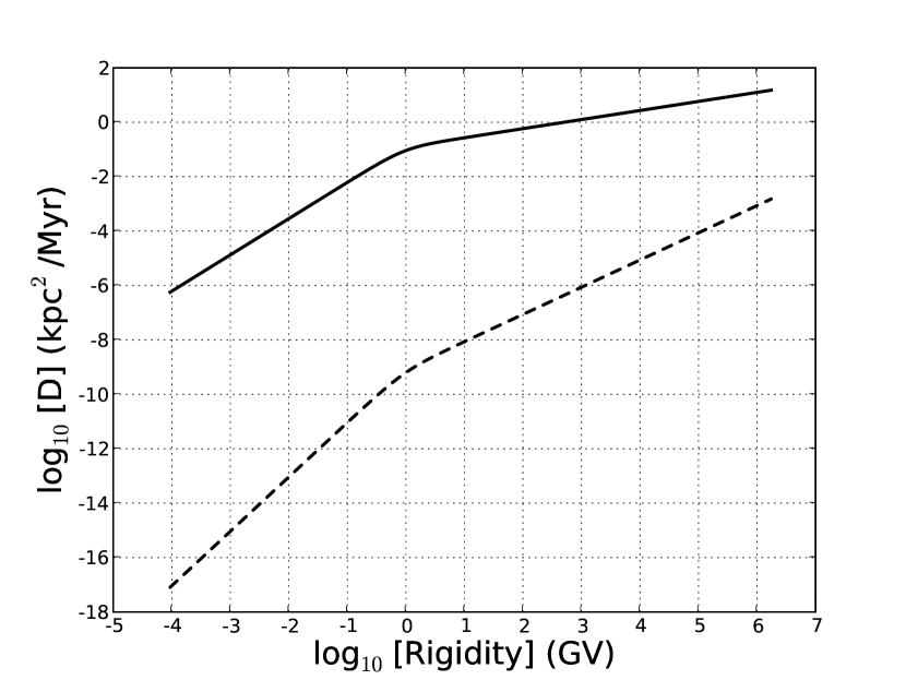
Figure 2.— Momentum-dependence of spatial diffusion coefficients for CR protons. Bohm diffusion (dashed curve) is implemented for the space inside the SNR shells ($D_{B}$); The Kolmogorov spectrum (solid curve) is employed for the space outside the shells for CR diffusion in the ISM ($D_{\mathrm{Kol}}$). A field $B=128$ $\mu$G is used for the $D_{B}$ plot. The normalization of $D_{\mathrm{Kol}}$ is taken from the calculation for the Galactic ridge by Ptuskin et al. (2006).

Simple diffusion of CR particles is incorporated in the simulation in a discretized manner. In each time step and each spatial grid in the 3-D simulation box, particles are exchanged between the adjacent boxels according to the particle momentum, location, and density gradient. The particle’s location determines which diffusion coefficient is used, and the simulation resolution is mainly determined by the boxel size and time step, $t_{\mathrm{step}}$, which are user-tunable.

3.2. Interaction Processes

The CR interaction processes considered include synchrotron radiation, bremsstrahlung, inverse-Compton scattering, and neutral pion decay. Energy changes from adiabatic effects and radiation, as well as Coulomb energy losses, are also included. All of these processes are treated in a fully space- and time-dependent fashion where the evolution of relevant parameters, such as the magnetic field and shell densities, are taken into account in each time step and boxel.

The details of the radiation processes can be found in Sturner et al. (1997) and Baring et al. (1999) but we note that, for IC emission, we only consider CR electrons colliding with a monoenergetic and isotropic photon field with an average energy density equal to that of the CMB field.

For hadronic interactions we employ the latest parametric proton-proton (p-p) model developed by Kamae et al. (2006). In this model, the total inclusive inelastic p-p cross-section includes the non-diffractive (with Feymann scaling violation) and diffractive components, plus the $\Delta(1232)$ and $Res(1600)$ resonance-excitation contributions important in the 10 MeV to 1 GeV range. This model alone can account for $\sim 20\%$ of the GeV $\gamma$ ray excess between the EGRET Galactic diffuse spectrum and previous model prediction using proton data in the solar system (Hunter et al., 1997).

3.2.1 Coulomb Losses

Coulomb losses for superthermal electrons are included in our model using equation (10) from Sturner et al. (1997), i.e.,

$$\dot{E}_{\mathrm{coul}}=-\left(\frac{4\pi e^{4}}{m_{e}c}\right)\left[\frac{\lambda(t)n_{\mathrm{SNR}}\eta^{e}_{\mathrm{He}}}{\beta_{e}}\right][\psi(t)-\psi^{\prime}(t)]\ ,$$ (5)

where $n_{\mathrm{SNR}}$ is the proton number density in a shocked shell, $\beta_{e}=v_{e}/c$ is the electron $\beta$, and $t$ is the time. The definitions of the other terms are in Sturner et al. (1997) but are not important for our discussion here. Equation (5) shows that Coulomb losses increase for large ambient densities and low electron speeds. As a shell of shocked material ages, Coulomb losses cause the low energy part of the superthermal electron distribution to become depleted, as indicated in Fig. 3. In all cases, Coulomb losses are insignifcant for protons.

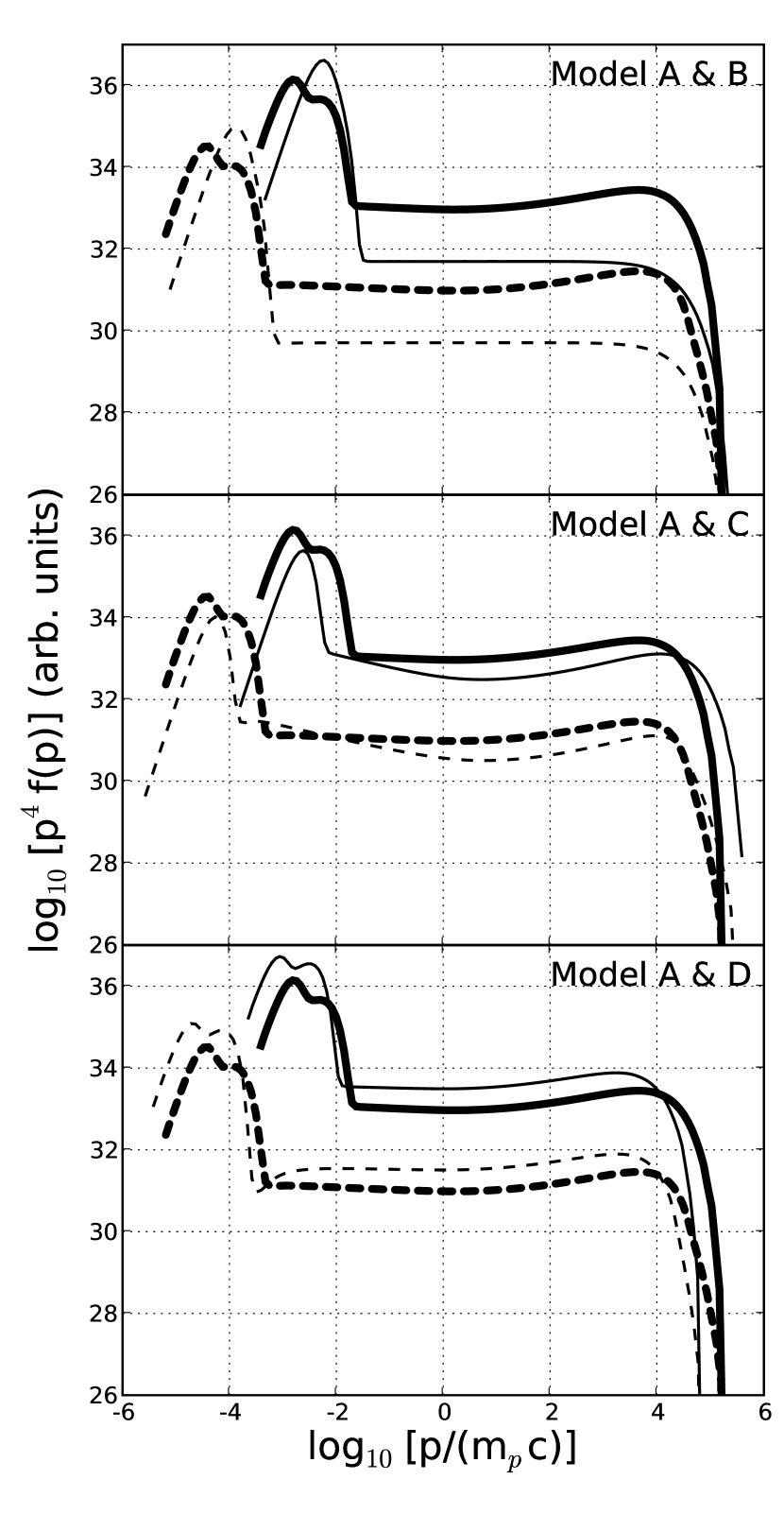
Figure 3.— CR spectra integrated over the whole SNR FS-CD region at 1000 yr, plotted as $p^{4}f(p)$, where f(p) is the phase space distribution function. In all panels, solid curves are protons and dashed curves are electrons. Also in all panels, the heavy curves are from Model A and these are compared to thin curves for Model B (top panel), Model C (middle panel), and Model D (bottom panel). Parameters for the various models are given in Table 1

4. Results

In this initial presentation of our 3-D simulation, we show results for a set of generic Type Ia SNR models where we vary the acceleration efficiency for DSA, $\epsilon_{\mathrm{acc}}=E_{\mathrm{CR}}/E_{\mathrm{SN}}$, and the ambient proton number density, $n_{p}$ (we assume the ISM is made of hydrogen). All of the other environmental and model parameters are kept constant with the values given in Sections 2.2.1 and 2.2.2.

Table 1SNR Model Parameters & Results

Model	$\epsilon_{\mathrm{acc}}$	$\chi_{\mathrm{inj}}$	$n_{p}$	$R_{\mathrm{FS}}$	$r_{\mathrm{tot}}$	$p_{\mathrm{max}}$	$\epsilon_{\mathrm{esc}}$	$F_{\mathrm{keV/TeV}}$	$F_{\mathrm{keV/TeV,MC}}$
			(cm-3)	(pc)		($10^{4}m_{p}c$)
A	0.75	3.70	1.0	4.67	10.66	1.37	0.27	1.24	0.97
B	0.01	4.27	1.0	5.14	4.04	1.77	0.0015	74.0	68.5
C	0.75	3.43	0.1	6.73	10.35	3.29	0.25	5.66	4.59
D	0.75	3.77	10.0	3.06	11.89	0.53	0.28	0.19	0.16

The values of $\epsilon_{\mathrm{acc}}$ and $n_{p}$ for the four models we compute are given in Table 1. We have included the injection efficiency, $\chi_{\mathrm{inj}}$, in Table 1 where $\chi_{\mathrm{inj}}$ determines $E_{\mathrm{CR}}/E_{\mathrm{SN}}$ and in practice we vary $\chi_{\mathrm{inj}}$ until we obtain the desired acceleration efficiency. We also show the fraction of $E_{\mathrm{SN}}$ that is in escaping particles, $\epsilon_{\mathrm{esc}}$. Model A is used as a reference for the other three and, for all of the models, the duration of each epoch is 50 yr so we have 20 shells in the SNR when it is 1000 yr old.

4.1. Electron and Proton Spectra

In Fig. 3 we show electron and proton phase-space distributions for the four models listed in Table 1. We plot $p^{4}f(p)$ to emphasize the spectral curvature at relativistic energies and the spectra are integrated over the entire shocked region between the FS and CD at the end of the simulation.

In the top panel, we compare Models A (efficient NL-DSA; bold lines) and B (inefficient DSA or TP acceleration; thin lines). The test-particle model shows flat electron and proton spectra at relativistic energies [$f(p)\propto p^{-4}$] with considerably lower fluxes at relativistic energies than Model A. The ‘thermal’ portions of the spectra show that the TP shock produces higher temperatures than in Model A, a characteristic feature of NL-DSA. The structure seen in the ‘thermal’ portions of the spectra comes about because these spectra are summed over the various shells and the ones produced early on have less efficient DSA and have a higher temperature than later shells.

In the middle and lower panels of Fig. 3 we keep $\epsilon_{\mathrm{acc}}=0.75$ but vary $n_{p}$; $n_{p}=0.1$ cm^-3 in the middle panel and $n_{p}=10$ cm^-3 in the lower panel. The important points for this comparison are: (i) the CR flux at relativistic energies scales approximately as $n_{p}$, as expected, (ii) the maximum proton momentum scales inversely as $n_{p}$ (see, for example, Baring et al., 1999), (iii) the electron cutoff energy also scales inversely as $n_{p}$ but is influenced by radiation losses and the dependence is weaker than for protons, and (iv) the shocked temperature scales inversely as $n_{p}$, although this is not immediately clear from the figures since the ‘thermal’ portions of the distributions are made up of contributions from a range of temperatures and densities.

Of course, other aspects of the hydrodynamics depend strongly on $n_{p}$. The radius of the SNR at $t_{\mathrm{SNR}}=1000$ yr is considerably greater for $n_{p}=0.1$ cm^-3 ($R_{\mathrm{FS}}=6.7$ pc) than for $n_{p}=10$ cm^-3 ($R_{\mathrm{FS}}=3.1$ pc). It is also expected that the FS will weaken faster with time for a denser upstream medium. However the strength, in terms of the efficiency of NL-DSA, also depends on the magnetic field and for the parameters used here, Model D has a larger compression ratio at $t_{\mathrm{SNR}}=1000$ yr ($r_{\mathrm{tot}}=11.9$) than Model A ($r_{\mathrm{tot}}=10.7$).

Coulomb losses also increase as $n_{p}$ increases and the dip which appears just above the thermal peak in the Model D electron spectrum (light dashed curve in lower panel) reflects Coulomb losses experienced by the superthermal electrons as they collide with the shocked thermal gas. Coulomb losses can be expected to be more pronounced in NL models because the larger compression ratio results in a larger post-shock density.

4.2. Spatial Variation and Escaping Flux

At any given time, the spatial variation of the CR spectrum can be calculated. Fig. 4 shows CR spectra of Model A at three different locations: (i) just behind the forward shock (solid lines); (ii) mid-way between the forward shock and the contact discontinuity (dashed lines); and (iii) at a distance of $d=9$ pc from the center of the SNR which is approximately $2-6$ pc beyond the FS, depending on the model (dotted lines). The heavy-weight curves are protons and the light-weight curves are electrons.

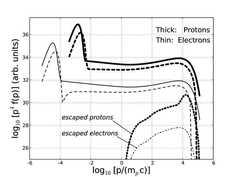
Figure 4.— Spatial variation of CR momentum distribution for Model A at t = 1000yr. The distribution is plotted at three locations: (i) just behind the FS (solid); (ii) mid-way between the FS and the CD (dashed); and (iii) at a distance of 9pc away from the SNR center (dash-dot). Thick lines are for protons and thin lines are for electrons.

Compared with the freshly accelerated electrons at location (i), many of the highest energy electrons are lost in the mid-point location (ii) mainly due to synchrotron losses with a small contribution from adiabatic losses. The protons show a smaller change which is due to adiabatic losses only.

At location (iii), only those CRs that escaped from the shock are present and their spectra lack a low energy component since low energy CRs remain trapped in the remnant. The hardness of the spectra at 9 pc from the center of the SNR reflects the strong momentum dependence of the escape probability and the spatial diffusion coefficients. The escape probability from the SNR increases with energy and high-energy CRs diffuse faster in the ISM.

4.3. Boardband Photon Spectrum

Once the particle spectra are determined, the photon emission can be calculated throughout the simulation box for arbitrary 3-dimensional distributions of matter and ambient photon fields.

We consider two simple matter distributions (i.e., ‘molecular clouds’) outside of the FS. The first is a spherical shell, concentric with the SNR where the inner and outer radii are equal to 9 and 10 pc, respectively. The second is a hemisphere centered at one side of the simulation box with radius = 3.2 pc (see Fig. 1). In both cases, the proton number density in the ‘molecular cloud’ is $n_{\mathrm{MC}}=10^{3}$ cm^-3 and the magnetic field is $B_{\mathrm{ISM}}=3$ $\mu$G, the same field as in the ISM. The entire simulation box is 20 pc on a side and is divided into $51\times 51\times 51$ boxels. The density in the ISM between the molecular clouds and the FS is $n_{p}$ and the photon field throughout the simulation box is the uniform CMB field for all models.

4.3.1 Emission from the SNR Shells

Fig. 5 shows the broadband photon emission for Models A to D integrated over the shocked SNR shells between the FS and CD. The bottom panel shows the total spectra while the upper three panels show the individual components from $\pi^{0}$-decay (solid), IC (dashed), synchrotron (dash-dotted), and bremsstrahlung (dotted) compared with Model A. Emission from CRs outside of the SNR is not shown.

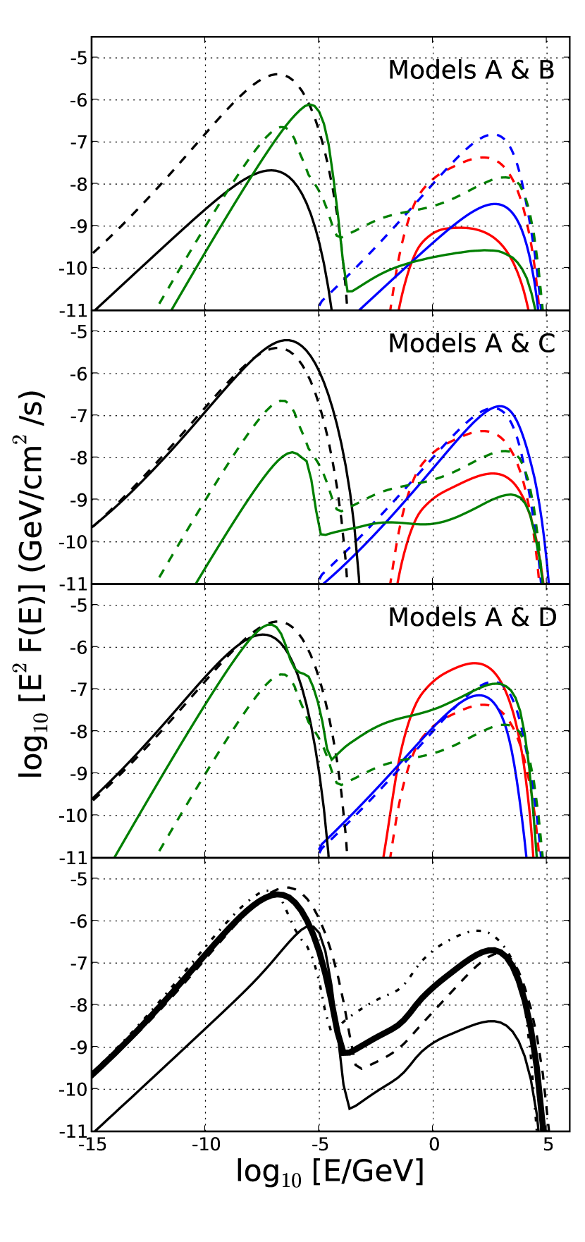
Figure 5.— Photon spectra of all four models integrated over the region from the CD to the FS. Upper three panels: Models B to D are compared to Model A and are split into individual components for different emission mechanisms: $\pi^{0}$-decay (red), IC (blue), bremsstrahlung (green) and synchrotron radiation (black). Solid lines represent spectra for Model B, C and D in each panel while Model A is shown as dashed lines. Bottom panel: The contributions from all mechanisms are summed for each model: Model A (thick solid), Model B (thin solid), Model C (dash) and Model D (dash-dot).

In Model A, the photon flux in the radio to X-ray energy range is dominated by synchrotron emission up to $\sim 100$ keV. The second largest contribution is from thermal bremsstrahlung which dominates between $\sim 100$ keV and $\sim 50$ MeV. Between $\sim 50$ MeV and $\sim 10$ GeV, pion-decay and IC compete. Beyond $\sim 10$ GeV, the emission is dominated by IC.

As seen in the A vs. B comparison panel, thermal bremsstrahlung plays an important role in the TP Model B and dominates synchrotron emission in the entire X-ray energy band. Thermal bremsstrahlung is strong in the TP model because the shocked temperatures are considerably higher than those in efficient DSA. The emission from synchrotron, IC, and pion-decay are all weak in the TP case as expected.

In the three NL Models A, C, and D, the acceleration efficiency is set at $\epsilon_{\mathrm{acc}}=0.75$, but the ambient density is varied with $n_{p}=1$, $0.1$ and $10$ cm^-3 respectively. In the X-ray band, the thermal bremsstrahlung scales approximately as $n_{p}^{2}$ and dominates synchrotron in Model D, where $n_{p}=10$ cm^-3.

Above $\sim 100$ MeV, the competition is mainly between IC and pion-decay but bremsstrahlung is also important for $n_{p}=10$ cm^-3. For Model C ($n_{p}=0.1$ cm^-3), both pion-decay and bremsstrahlung are suppressed relative to IC. For Model D, pion-decay dominates until near the maximum energies where bremsstrahlung becomes comparable.

4.3.2 Emission from a Shell ‘Molecular Cloud’

We first consider the shell of external material centered with the SNR. Protons and electrons which have sufficiently high energy and, therefore, long diffusion lengths can escape from the FS and enter the ISM. These CRs also interact with the ambient ISM material of density $n_{p}$ and the CMB radiation.

In Fig. 6 we show the photon spectra from the molecular cloud shell for Models A–D in the same representation as Fig. 5 but now integrated over the molecular cloudvolume, all calculated at $t_{\mathrm{SNR}}=1000$ yr. As expected, these spectra are considerably harder than their counterparts inside the remnant. The escape of CRs from the forward shock during acceleration depends on the diffusion coefficient and the strong momentum dependence of the Bohm diffusion coefficient, $D_{B}$, favors the escape of the highest energy particles. Once in the ISM, the relativistic CRs diffuse with a diffusion coefficient $D_{\mathrm{Kol}}\propto p^{1/3}$, hardening the spectrum even more, as shown in Fig. 4. The photon spectra reflect the hard particle spectra.

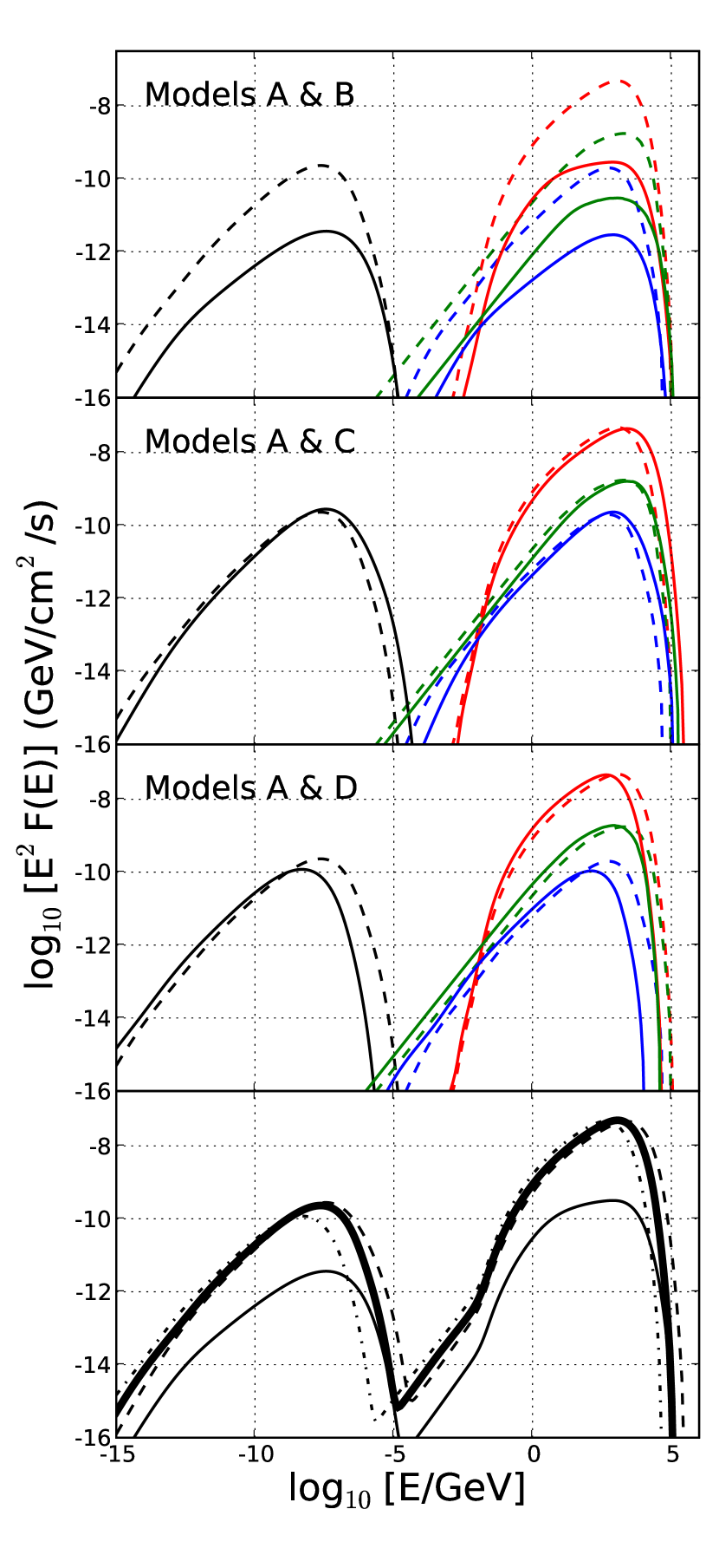
Figure 6.— Same as Fig. 5 but the photon spectra are now integrated over the shell molecular cloud volume. The strong momentum dependent diffusion results in hard spectra and a change in the relative dominance between the emission mechanisms, compared to spectra integrated over the SNR.

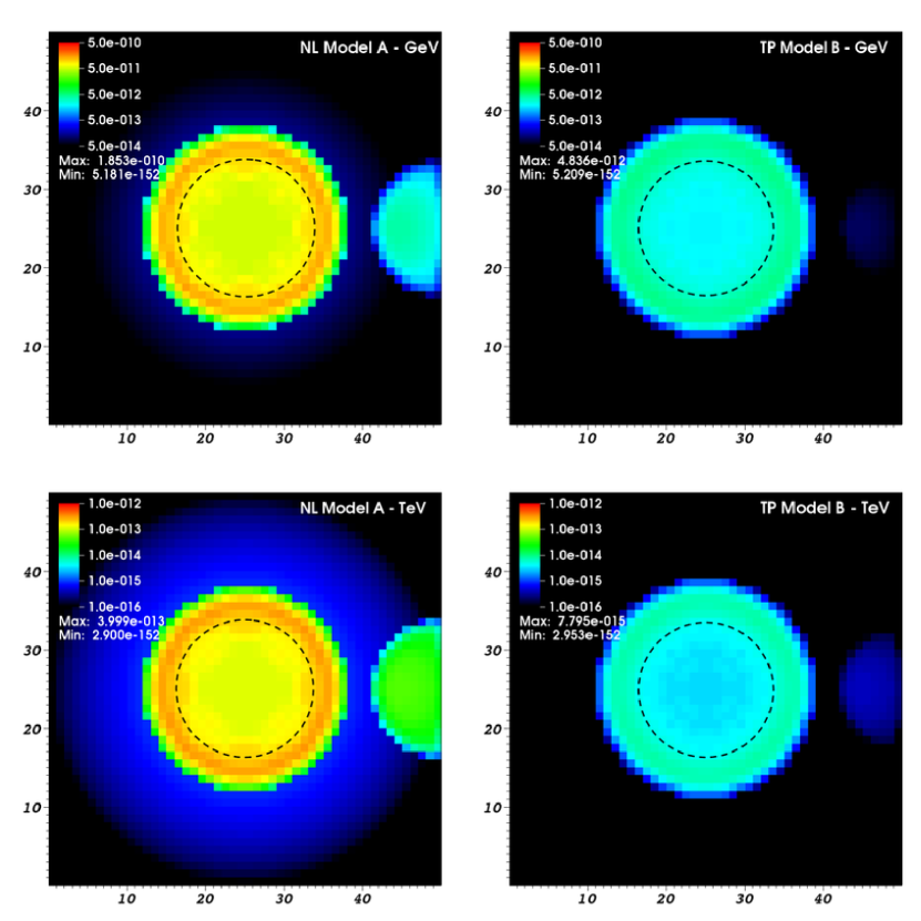
Figure 7.— Photon flux maps projected along the line-of-sight for Model A (left panels) and Model B (right panels), with a hemisphere molecular cloud centered at pixel coordinate (50,25,25) with a radius of 3.2 pc. The horizontal and virtical scales are in pixels where the pixel size is 0.38 pc $\times$ 0.38 pc. The upper panels are integrated over the energy range $1-300$ GeV, while the bottom panels are integrated over energies $E_{\gamma}\geq 1$ TeV. The color scale is logarithmic in $\log(N_{\gamma}/\mathrm{cm}^{2}/\mathrm{s})$. The dashed circle in each panel indicates the position of the contact discontinuity.

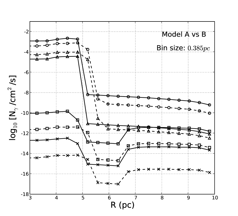
Figure 8.— Line-of-sight emission profiles in the radial direction from the SNR center at $R=0$ to the hemispheric ‘molecular cloud’ centered at $R=10$ pc. Results for Model A (solid curves) and Model B (dashed curves) are displayed. Markers represent the centers of the cubic spatial bins which are $0.385$ pc on a side. Four wavebands are considered - (i) Soft X-rays from 1 to 5 keV (circle); (ii) Hard X-rays from 5 to 10 keV (triangle); (iii) 1 to 300 GeV $\gamma$-rays (square) and (iv) $\gamma$-rays with energy above 1 TeV (cross). The vertical axis shows the photon flux in log($N_{\gamma}$/cm²/s) for each pixel bin.

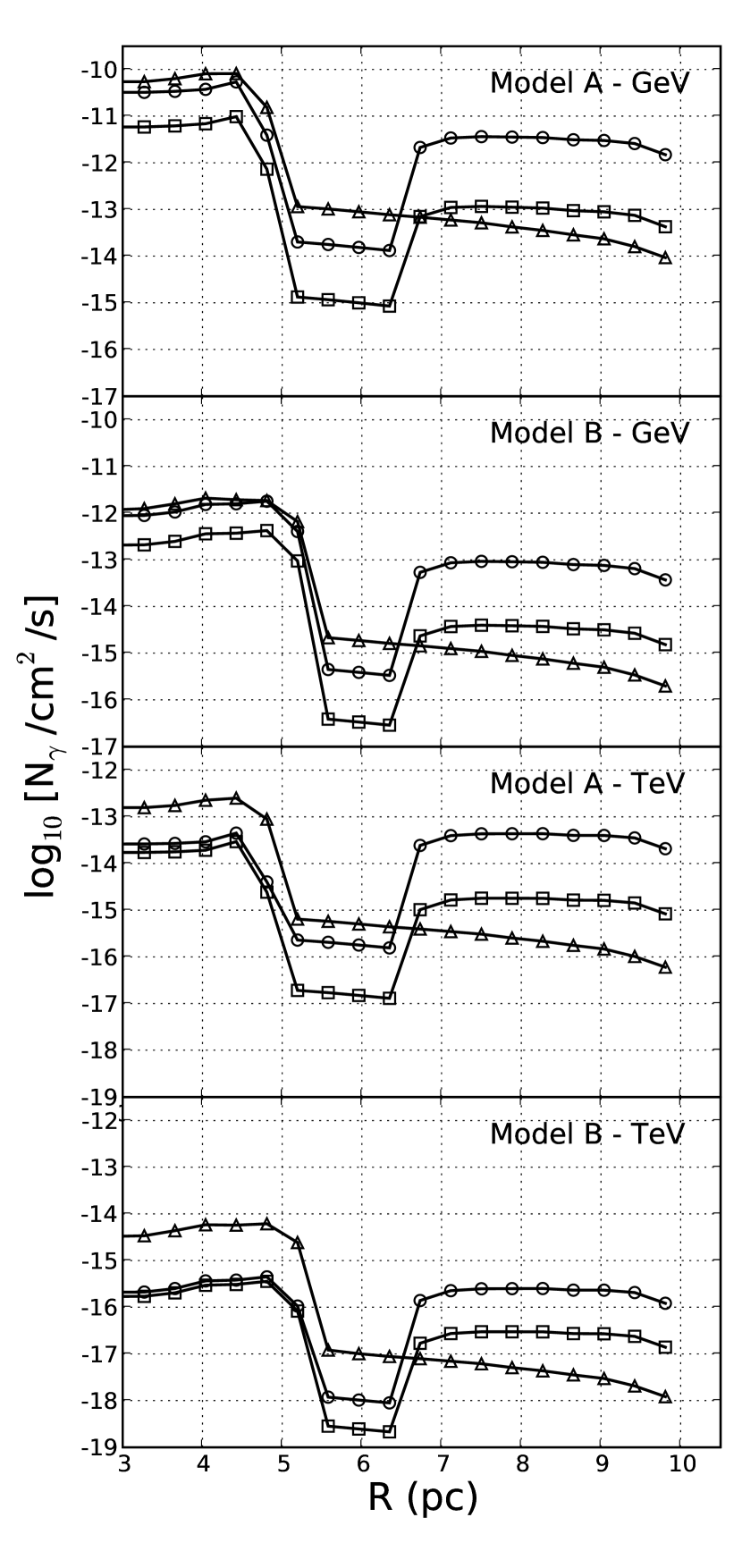
Figure 9.— Same as Fig. 8 with individual emission processes shown, i.e., pion-decay (circles), IC (triangles), and bremsstrahlung (squares). Synchrotron emission has a negligible flux in the $\gamma$-ray energy band.

With a number density of $n_{\mathrm{MC}}=10^{3}$ cm^-3, and a column density of $n_{\mathrm{Col}}\sim 10^{21-22}$  cm^-2 in the ‘molecular cloud,’ $\pi^{0}$-decay is the main $\gamma$-ray source for all models, followed by relativistic bremsstrahlung and then IC emission, as shown in Fig. 6. For Models A, B, C and D, the separation between the FS and the inner edge of the MC is found to be around $4.3$, $3.8$, $2.3$ and $5.9$ pc respectively at $t=1000$ yr.

For the environmental parameters studied here, the emission at all wavebands from the molecular cloud is weaker than that from the SNR shell, but the difference depends on the photon energy. With the assumption $B_{\mathrm{MC}}=3$ $\mu$G, the X-ray synchrotron flux from the molecular cloud stays at the ISM level and will be difficult to detect. The GeV $\gamma$-ray flux is more model-dependent and the flux stays around a factor of 10–100 smaller than the flux from the SNR. For the TeV flux, which is detected by atmospheric Cherenkov telescopes, the molecular cloud emission is about $1-10\%$ of that from the SNR.

4.4. Boardband Images and Projected Emission Profiles

Multi-wavelength projection maps are useful for studying the energy-dependent morphology of SNRs. We use our hemispherical ‘molecular cloud’ example (Fig. 1) to calculate 2-D projection maps in various energy bands at $t_{\mathrm{SNR}}=1000$ yr for Models A and B. After the photon emissivity is calculated in each boxel in the 3-D simulation box, we perform a line-of-sight projection through the box. We choose four energy bands: (i) soft X-rays with $E_{\gamma}=1-5$ keV; (ii) hard X-rays with $E_{\gamma}=5-10$ keV; (iii) $E_{\gamma}=1-300$ GeV; and (iv) $E_{\gamma}>1$ TeV. The parameters we use result in a column density of $\sim 10^{21}$ cm^-2 for the cloud, which is small enough to ignore in the present context.

Fig. 7 shows the $\gamma$-ray projected flux maps in $\log(N_{\gamma}/\mathrm{cm}^{2}/\mathrm{s})$ at a source distance of $D_{\mathrm{SNR}}=1$ kpc for Models A (NL) and B (TP) in the GeV and TeV bands [i.e., bands (iii) and (iv)]. The color scales are different for the GeV and TeV images, but the spatial resolution is the same. The difference between the example with efficient DSA (left panels) and the test-particle case (right panels) is mainly one of intensity if only GeV-TeV emission is concerned. In both cases, the brightest regions of the SNR are considerably brighter than the cloud and for the test-particle case (Model B), the cloud is almost invisible on these scales. For the SNR in both the NL and TP cases, the region between the CD and FS clearly shows up in the maps even with the projection through the remnant. There is also a clear limb darkening effect from projection seen at the edge of both remnants and at the edge of the cloud in the NL case. At the molecular cloud, however, there is no noticable drop in intensity towards the center of the cloud as occurs for the SNR.

These details, of course, depend on the particular parameters we have chosen but some general statements can be made. Unless there is a source of soft photons associated with the external material, the brightness of the external material (MC) compared to the SNR, the $I_{\mathrm{MC}}/I_{\mathrm{SNR}}$ ratio, will be independent of the density ratio $n_{\mathrm{MC}}/n_{p}$ if IC dominates the GeV-TeV emission. If pion-decay or bremsstrahlung dominate, the $I_{\mathrm{MC}}/I_{\mathrm{SNR}}$ ratio will scale approximately as the first power of the density ratio, $n_{\mathrm{MC}}/n_{p}$. In all cases, $I_{\mathrm{MC}}/I_{\mathrm{SNR}}$ will decrease with the distance the external material is from the FS. Another important result, which is implicit in Fig. 7 and important for comparing pion-decay and IC emission, is that emission from the SNR and the external material must be considered together. To first order, an increase in acceleration efficiency or ambient matter density not solely associated with the cloud, $n_{p}$, will leave $I_{\mathrm{MC}}/I_{\mathrm{SNR}}$ unchanged.

In Fig. 8 we show emission calculated along a horizontal line from the center of the remnant at $R=0$ across the molecular cloud for all four energy bands. These fluxes are determined, as are the 2-D maps, by summing the emission from each boxel along a line-of-sight. The plateaus on the left hand side of the plot within $R\lesssim 5$ pc show emission from the SNR. The subtle increase of the projected flux with $R$ in this region is the result of projection through the shell of material between the CD and the FS. Beyond $R\sim 5$ pc, the fluxes drop abruptly to the ISM level. Here, escaping CRs stream through the ISM with a large diffusion coefficient $D_{\mathrm{Kol}}$. At $R\sim 6.8$ pc, the CRs impact the hemisphere ‘molecular cloud’ with $n_{\mathrm{MC}}=10^{3}$ cm^-3 and the fluxes for energy bins (iii) and (iv) increase by almost 2 orders of magnitude from the ISM level. These photons are mainly from pion-decay. There is no increase at the edge of the cloud for energy bins (i) and (ii) since this emission is totally from synchrotron and we have assumed the field in the molecular cloud equals the ISM field, $B_{\mathrm{MC}}=B_{\mathrm{ISM}}$.

Fig. 9 shows the emission profiles in bands (iii) and (iv) for Models A and B separated into individual emission mechanisms. While the total fluxes at these energies depend strongly on acceleration efficiency, the $I_{\mathrm{MC}}/I_{\mathrm{SNR}}$ ratio is much less sensitive to $\epsilon_{\mathrm{acc}}$, as mentioned above. There is no increase in IC emission at the edge of the cloud near $R\sim 6.9$ pc since we only consider electron scattering off the CMB. Unless there is an additional source of photons associated with the external material, IC will be strongly suppressed relative to pion-decay in external material.

5. Summary and Conclusions

We have introduced a 3-D simulation of an evolving SNR where the nonlinear acceleration of CRs is coupled to the SNR evolution. The model follows the diffusion and interaction of CRs within the spherically symmetric remnant, as well as high-energy CRs that escape from the forward shock and diffuse into the surrounding medium. For any set of model and environmental parameters, and for arbitrary distributions of matter surrounding the remnant, we can calculate broadband photon spectra and obtain line-of-sight projections and morphologies that will allow for efficient comparisons with observations in various energy bands.

We have illustrated the capabilities of this simulation with several models that differ from each other in the CR acceleration efficiency, $\epsilon_{\mathrm{acc}}$, the ambient ISM proton density, $n_{p}$, and the matter distribution of a ‘molecular cloud’ external to the SNR. Of course, all of the results discussed here assume particular values for parameters, such as a shocked electron to proton temperature ratio $T_{e}/T_{p}=1$ and an electron/proton ratio at relativistic energies $(e/p)_{\mathrm{rel}}=0.01$. These parameters are critical for understanding DSA and applying the mechanism to astrophysical sources yet they are poorly constrained by both observations and theory. For instance, the value of $T_{e}/T_{p}$ determines the importance of bremsstrahlung compared to synchrotron in the X-ray range and also strongly influences the thermal X-ray line spectra (Ellison et al., 2007). The $(e/p)_{\mathrm{rel}}$ ratio is the most important factor after the ambient density determining the relative intensity of IC and pion-decay emission at GeV-TeV energies. The confirmation of CR ion production in SNRs depends on this parameter.

Other important parameters of DSA that remain uncertain are the injection and acceleration efficiencies, the amount of magnetic compression and amplification that occurs, and the diffusion coefficient of escaping particles as they leave the shock, which must differ substantially from Bohm diffusion (e.g., Blasi et al., 2007; Ellison & Vladimirov, 2008). Due to the still limited dynamic range of particle-in-cell simulations, and the lack of strong, nonlinear shocks producing relativistic particles in the heliosphere, we believe young SNRs are the best ‘laboratory’ for studying NL-DSA. Broadband observations matched against self-consistent nonlinear models currently provide the best constraints on these important parameters.

There are three important aspects of our 3-D simulation that are new and extend the large body of existing work on DSA in SNRs. One is that the simulation consistently models high-energy CRs that escape from the forward shock of the SNR with the evolution of the SNR itself. In NL-DSA, the fraction of total explosion energy that ends up in escaping particles can be large (see Table 1) and we believe this is the first work to include these particles in a coherent emission model. Second, the 3-D simulation box allows for the modeling of CR interactions in arbitrary mass distributions outside of the SNR. This feature is essential for producing 2-D projection maps that can be compared with current and future observations. These maps, tuned to match the instrument response of telescopes, will serve to help determine the importance of pre-SN shells and/or nearby molecular clouds in producing $\gamma$-ray emission. Third, the simulation platform is extremely flexible making it straightforward to add important effects not present in this preliminary model. These generalizations include shock acceleration and heating at the reverse shock as well as the forward shock, pre-SN winds for Type II SNe, various forms for particle diffusion in the ISM, production and interaction of heavy CR ions, and a parameterized representation of magnetic field amplification.

Another physical effect that may importantly influence the photon spectrum is anisotropy from angular-dependent interactions. These include an angular-dependent neutral pion production cross-section (Karlsson & Kamae, 2007) and anisotropic IC scattering with photon fields other than the CMB (Moskalenko & Strong, 2000). Preliminary results show that anisotropies can change the spectral shape and flux of the observed photons drastically. When anisotropic interactions are implemented, the projection maps we calculate will show how the observed flux depends on the orientation of the FS and molecular cloud with respect to the line-of-sight. We leave this issue to future studies.

Finally, in addition to modeling the photon emission from SNRs, our model can also determine the total contribution of CR ions and electrons injected into the Galaxy from an individual SNe over its lifetime. This can serve as input to Galaxy-scale propagation models (for example, GALPROP, Strong et al., 2007) and also add to our knowledge on the Galactic $\gamma$-ray diffuse emission.

References

- Aharonian et al. (2005) Aharonian F., Akhperjanian A.G., Bazer-Bachi A.R., et al., Jul. 2005, A&A, 437, L7
- Aharonian et al. (2006) Aharonian F., Akhperjanian A.G., Bazer-Bachi A.R., et al., Apr. 2006, A&A, 449, 223
- Aharonian et al. (2008) Aharonian F., Akhperjanian A.G., Bazer-Bachi A.R., et al., Apr. 2008, A&A, 481, 401
- Albert et al. (2007) Albert J., Aliu E., Anderhub H., et al., Aug. 2007, ApJ, 664, L87
- Amato & Blasi (2005) Amato E., Blasi P., Nov. 2005, MNRAS, 364, L76
- Amato & Blasi (2006) Amato E., Blasi P., Sep. 2006, MNRAS, 371, 1251
- Bamba et al. (2003) Bamba A., Yamazaki R., Ueno M., Koyama K., Jun. 2003, ApJ, 589, 827
- Baring et al. (1999) Baring M.G., Ellison D.C., Reynolds S.P., Grenier I.A., Goret P., 1999, ApJ, 513, 311
- Bell & Lucek (2001) Bell A.R., Lucek S.G., 2001, MNRAS, 321, 433
- Berezhko & Ellison (1999) Berezhko E.G., Ellison D.C., 1999, ApJ, 526, 385
- Berezhko & Völk (2006) Berezhko E.G., Völk H.J., Jun. 2006, A&A, 451, 981
- Berezhko et al. (1996) Berezhko E.G., Elshin V.K., Ksenofontov L.T., Jan. 1996, Journal of Experimental and Theoretical Physics, 82, 1
- Berezhko et al. (2003) Berezhko E.G., Ksenofontov L.T., Völk H.J., Dec. 2003, A&A, 412, L11
- Blandford & Eichler (1987) Blandford R., Eichler D., Oct. 1987, Physics Reports, 154, 1
- Blasi et al. (2005) Blasi P., Gabici S., Vannoni G., Aug. 2005, MNRAS, 361, 907
- Blasi et al. (2007) Blasi P., Amato E., Caprioli D., Mar. 2007, MNRAS, 375, 1471
- Chevalier et al. (1978) Chevalier, R. A., Oegerle, W. R. & Scott, J. S., 1978, ApJ, 222, 527-536
- Cowsik & Sarkar (1980) Cowsik R., Sarkar S., Jun. 1980, MNRAS, 191, 855
- Drury (1983) Drury L.O., Aug. 1983, Reports of Progress in Physics, 46, 973
- Ellison & Cassam-Chenaï (2005) Ellison D.C., Cassam-Chenaï G., Oct. 2005, ApJ, 632, 920
- Ellison & Vladimirov (2008) Ellison D.C., Vladimirov A., Jan. 2008, ApJ, 673, L47
- Ellison et al. (2004) Ellison D.C., Decourchelle A., Ballet J., 2004, A&A, 413, 189
- Ellison et al. (2007) Ellison D.C., Patnaude D.J., Slane P., Blasi P., Gabici S., Jun. 2007, ApJ, 661, 879
- Erlykin & Wolfendale (1999) Erlykin A.D., Wolfendale A.W., Oct. 1999, A&A, 350, L1
- Gabici & Aharonian (2007) Gabici S., Aharonian F.A., Aug. 2007, ApJ, 665, L131
- Hillas (2005) Hillas A.M., May 2005, Journal of Physics G Nuclear Physics, 31, 95
- Hoppe et al. (2007) Hoppe S., Lemoine-Goumard M., for the H. E. S. S. Collaboration, Sep. 2007, ArXiv e-prints, 709
- Hunter et al. (1997) Hunter S.D., Bertsch D.L., Catelli J.R., et al., May 1997, ApJ, 481, 205
- Jones & Ellison (1991) Jones F.C., Ellison D.C., 1991, Space Science Reviews, 58, 259
- Kamae et al. (2006) Kamae T., Karlsson N., Mizuno T., Abe T., Koi T., Aug. 2006, ApJ, 647, 692
- Karlsson & Kamae (2007) Karlsson N., Kamae T., Sep. 2007, ArXiv e-prints, 709
- Kobayashi et al. (2001) Kobayashi T., Nishimura J., Komori Y., Yoshida K., 2001, Advances in Space Research, 27, 653
- Koyama et al. (1995) Koyama K., Petre R., Gotthelf E.V., et al., Nov. 1995, Nature, 378, 255
- Moskalenko & Strong (2000) Moskalenko I.V., Strong A.W., Jan. 2000, ApJ, 528, 357
- Pohl et al. (2005) Pohl M., Yan H., Lazarian A., Jun. 2005, ApJ, 626, L101
- Ptuskin et al. (2006) Ptuskin V.S., Moskalenko I.V., Jones F.C., Strong A.W., Zirakashvili V.N., May 2006, ApJ, 642, 902
- Reynolds & Ellison (1992) Reynolds S.P., Ellison D.C., Nov. 1992, ApJ, 399, L75
- Rho et al. (2002) Rho J., Dyer K.K., Borkowski K.J., Reynolds S.P., Dec. 2002, ApJ, 581, 1116
- Strong et al. (2007) Strong A.W., Moskalenko I.V., Ptuskin V.S., Nov. 2007, Annual Review of Nuclear and Particle Science, 57, 285
- Sturner et al. (1997) Sturner S.J., Skibo J.G., Dermer C.D., Mattox J.R., Dec. 1997, ApJ, 490, 619
- Torres et al. (2008) Torres, D. F., Rodriguez Marrero, A. Y., & de Cea del Pozo, E., 2008, MNRAS, preprint
- Uchiyama et al. (2007) Uchiyama Y., Aharonian F.A., Tanaka T., Takahashi T., Maeda Y., Oct. 2007, Nature, 449, 576
- Ueno et al. (2007) Ueno M., Sato R., Kataoka J., et al., Jan. 2007, PASJ, 59, 171
- Völk et al. (2002) Völk H.J., Berezhko E.G., Ksenofontov L.T., Rowell G.P., Dec. 2002, A&A, 396, 649
- VERITAS Collaboration: T. B. Humensky (2007) VERITAS Collaboration: T. B. Humensky, Sep. 2007, ArXiv e-prints, 709
- Vladimirov et al. (2006) Vladimirov A., Ellison D.C., Bykov A., Dec. 2006, ApJ, 652, 1246
- Zirakashvili & Ptuskin (2008) Zirakashvili V.N., Ptuskin V.S., Jan. 2008, ArXiv e-prints, 801