Cluster-based density-functional approach to quantum transport
through molecular and atomic contacts

Abstract

We present a cluster-based density-functional approach to model charge transport through molecular and atomic contacts. The electronic structure of the contacts is determined in the framework of density functional theory, and the parameters needed to describe transport are extracted from finite clusters. A similar procedure, restricted to nearest-neighbor interactions in the electrodes, has been presented by Damle et al. [Chem. Phys. 281, 171 (2002)]. Here, we show how to systematically improve the description of the electrodes by extracting bulk parameters from sufficiently large metal clusters. In this way we avoid problems arising from the use of nonorthogonal basis functions. For demonstration we apply our method to electron transport through Au contacts with various atomic-chain configurations and to a single-atom contact of Al.

I Introduction

Advances in the experimental techniques for manipulating and contacting atomic-sized objects have turned the vision of molecular-scale electronic circuits into a realistic goal.Nazin et al. (2003); Nitzan and Ratner (2003); Tao (2006); Lindsay and Ratner (2007); Akkerman and de Boer (2008) This has intensified the interdisciplinary efforts to study charge transport in nanostructures. Ideally, the circuits would be constructed in a bottom-up approach with functional units and all the wiring on the molecular scale. To approach the goal, present-day experiments in the area of molecular electronics concentrate on measuring the current-voltage response of single molecules in contact to metallic electrodes. In these studies, also purely metallic atomic contacts and wires serve as important reference systems.Agraït et al. (2003)

In order to support the experiments and to stimulate further technological advance, theoretical modeling of atomic-scale charge transport is needed. Here one faces the challenge to describe infinitely extended, low-symmetry quantum systems that may, in addition, be far from equilibrium and involve strong electronic correlations. While a complete theoretical understanding is still lacking, sophisticated ab-initio methods have been developed for approximate but parameter-free numerical simulations. In order to study the prototypical metal-molecule-metal systems or metallic atomic contacts, many groups use density functional theory (DFT) combined with nonequilibrium Green’s function (NEGF) techniques.Taylor et al. (2001); Xue et al. (2001); Damle et al. (2001); Brandbyge et al. (2002); Palacios et al. (2002); Heurich et al. (2002); Fujimoto and Hirose (2003); Wortmann et al. (2002); Jelínek et al. (2003); Havu et al. (2004); Tada et al. (2004); Evers et al. (2004); Khomyakov and Brocks (2004); Calzolari et al. (2004); Thygesen and Jacobsen (2005); Rocha et al. (2006) Some shortcomings related to the use of DFT in this context have been pointed out, and solutions are being sought.Ferretti et al. (2005); Toher et al. (2005); Darancet et al. (2007); Thygesen and Rubio (2008) On the other hand, from a practical point of view DFT presently appears to be one of the most useful ab-initio electronic structure methods, since studies of quantum transport require dealing with a large number of atoms. Furthermore the metal-molecule-metal contacts are hybrid systems, where the central regions frequently behave rather insulator-like, while the electrodes are metallic. For more complete discussions we refer to Refs. Cuevas et al., 2003; Pecchia and Di Carlo, 2004; Koentopp et al., 2008.

The DFT approaches can mainly be divided into two types. In the first one, atomic-sized contacts are modelled by periodically repeated supercells, and computer codes developed for solid-state calculations are employed.Brandbyge et al. (2002); Thygesen and Jacobsen (2005); Rocha et al. (2006) The use of periodic boundary conditions facilitates the electrode description. However, the conductance is determined for an array of parallel junctions and may be affected by artifical interactions between them. The second type is based on finite clusters and originates more from the chemistry community.Damle et al. (2001); Xue et al. (2001); Palacios et al. (2002); Heurich et al. (2002); Tada et al. (2004) It has the advantage that genuinely single-atom or single-molecule contacts are described, and it makes possible investigations of molecules of large transverse extent. The drawback is typically the description of the electrode, since it is difficult to treat bulk properties based on finite clusters. Furthermore the coupling between the device region and the electrode can be complicated by finite-size and surface mismatch effects.

To arrive at an ab-initio DFT description it is necessary to treat the whole system consistently by using the same basis set and exchange-correlation functional everywhere. The problem of the cluster-based approaches regarding the electrodes is apparent, for example, from the work of Refs. Xue et al., 2001; Palacios et al., 2002; Heurich et al., 2002, where the authors resort to a separate tight-binding parameterization obtained from the literature.Papaconstantopoulos (1986) Damle et al. proposed to resolve this issue by extracting electrode parameters from finite clusters computed within DFT.Damle et al. (2001, 2002) However, their treatment of the electrodes should be seen as a first approximation, since only couplings between nearest neighbor atoms were considered. Furthermore, they finally use energy-independent self-energies, which is well-justified only for electrode materials with a constant density of states (DOS) near the Fermi energy.

In this work we present a cluster-based DFT approach for the atomistic description of quantum transport. We follow the ideas of Ref. Damle et al., 2002, but place special emphasis on the treatment of the electrodes. In particular, we show that extracting electrode parameters from small metal clusters can lead to an unphysical behavior of the overlap of the nonorthogonal basis functions in $k$-space. The description of the electrodes can be improved systematically by employing metal clusters of increasing size. Our implemenation is based on the quantum-chemistry package TURBOMOLE, which allows us to treat clusters of several hundred atoms. In this way we obtain an ab-initio formulation of quantum transport in atomic-sized contacts, where the whole system is treated on an equal footing. It has the advantage that we can employ high-quality quantum-chemical Gaussian basis sets, which are well-tested for isolated systems.

The theoretical framework of our approach is presented in Sec. II. Several technical details, related to the use of nonorthogonal basis functions and the electrode treatment can be found in Apps. A and B. To demonstrate the power of our methods we study in Sec. III the transport properties of atomic contacts of Au and Al. The choice of these materials is motivated by the fact that Au exhibits a rather energy-independent DOS near the Fermi energy, while Al does not. Furthermore, for these systems we can compare our results to the literature. We find good agreement, and demonstrate the robustness of our results. Further applications have been presented in Refs. Wohlthat et al., 2007; Viljas et al., 2007; Wohlthat et al., 2008; Pauly et al., 2008, . We summarize our results in Sec. IV.

II Theoretical approach

II.1 Electronic structure

Our ab-initio calculations are based on the implementation of DFT in TURBOMOLE 5.9.Ahlrichs et al. (1989) By ab-initio we mean that the simulations require no system-specific parameters. Self-consistent DFT calculations of large systems are generally very time-consuming. TURBOMOLE, however, is specialized in handling such systems, and offers several possibilities to reduce the computational effort. Thus, one can exploit point group symmetries, including non-Abelian ones. In this way, the calculations speed up by a factor given by the order of the point group. Further options are the “resolution of the identity in $J$” (RI-$J$)Eichkorn et al. (1995, 1997) and the “multipole-accelerated resolution of the identity $J$” (MARI-$J$),Sierka et al. (2003) which are both implemented in the ridft module of TURBOMOLE. The approximations help to reduce the effort to compute the Coulomb integrals $J$, which are particularly expensive to evaluate. With the help of the RI-$J$ approximation, known also under the name “density fitting”, the four-center-two-electron integrals can be expressed as three-center-two-electron ones.Koch and Holthausen (2001) Calculations are faster by a factor of 10-100 as compared to standard DFT, but equally accurate. The MARI-$J$ technique concerns the Coulomb interactions between distant atoms. They are divided into a near-field and a far-field part, where the near field is treated with RI-$J$ and the far field by a multipole approximation. Compared to RI-$J$, it can accelerate the calculations by another factor of 2-7.Sierka et al. (2003) DFT requires the choice of an exchange-correlation functional.Fiolhais et al. (2003) We select the generalized-gradient functional BP86,Becke (1988); Perdew (1986) which is known to yield good results for large metal clusters.Ahlrichs and Elliott (1999); Furche et al. (2002); Köhn et al. (2001); Nava et al. (2003) To express the orbital wave functions, Gaussian basis sets of split-valence-plus-polarization (SVP) quality are used,Schäfer et al. (1992); Eichkorn et al. (1995, 1997) which are the TURBOMOLE standard. Within the closed-shell formalism of DFT, total energies of all our clusters are converged to a precision better than $10^{-6}$ a.u. In order to obtain ground-state structures, the total energy needs to be minimized with respect to the nuclear coordinates. We perform such geometry optimizations or “relaxations” until the maximum norm of the Cartesian gradient has fallen below $10^{-4}$ a.u.

II.2 Transport formalism

We compute transport properties of atomic-sized contacts using the Landauer-Büttiker theory and Green’s functions expressed in a local, nonorthogonal basis.Xue et al. (2002); Viljas et al. (2005) The local atomic basis allows us to partition the basis states $\left|i,\alpha\right\rangle$ into left ($L$), central ($C$), and right ($R$) ones, according to a division of the contact geometry. In the basis states, $\alpha$ refers to the type of orbital at the position of atom $i$. For reasons of brevity we will frequently suppress the orbital index. The Hamiltonian (or Kohn-Sham) matrix $H_{i\alpha,j\beta}=\left\langle i,\alpha\right|H\left|j,\beta\right\rangle$, and analogously the overlap matrix $S_{i\alpha,j\beta}=\left\langle i,\alpha\right.\left|j,\beta\right\rangle$, can thus be written in block form,

$$H=\left(\begin{array}[]{ccc}H_{LL}&H_{LC}&0\\ H_{CL}&H_{CC}&H_{CR}\\ 0&H_{RC}&H_{RR}\end{array}\right).$$ (1)

Both $S$ and $H$ are real-valued and are hence symmetric. In addition, we assume the $C$ region to be large enough to have $S_{LR}=H_{LR}=0$. Within the Landauer-Büttiker theory,Datta (2005) the linear conductance can be expressed as

$$G=\frac{2e^{2}}{h}\int dE\left[-\frac{\partial}{\partial E}f(E,T)\right]\tau(E),$$ (2)

where $f(E,T)=\left\{\exp\left[\left(E-\mu\right)/\left(k_{B}T\right)\right]+1\right\}^{-1}$ is the Fermi function, and the chemical potential $\mu$ is approximately equal to the Fermi energy $E_{F}$, $\mu\approx E_{F}$. Using the standard NEGF technique, the transmission function is given by

$$\tau(E)=\mathrm{Tr}\left[\Gamma_{L}(E)G_{CC}^{r}(E)\Gamma_{R}(E)G_{CC}^{a}(E)\right]=\mathrm{Tr}\left[t^{\dagger}(E)t(E)\right]$$ (3)

with the transmission matrix

$$t(E)=\sqrt{\Gamma_{R}(E)}G_{CC}^{a}(E)\sqrt{\Gamma_{L}(E)}.$$ (4)

Here we define the Green’s functions

$$G_{CC}^{r}(E)=\left[ES_{CC}-H_{CC}-\Sigma_{L}^{r}(E)-\Sigma_{R}^{r}(E)\right]^{-1}$$ (5)

and $G_{CC}^{a}=\left[G_{CC}^{r}\right]^{\dagger}$, the self-energies

$$\Sigma_{X}^{r}(E)=\left(H_{CX}-ES_{CX}\right)g_{XX}^{r}(E)\left(H_{XC}-ES_{XC}\right),$$ (6)

and the scattering-rate matrices

$$\Gamma_{X}(E)=-2\mathrm{Im}\left[\Sigma_{X}^{r}(E)\right],$$ (7)

where $g_{XX}^{r}$ is the electrode Green’s function for lead $X=L$,$R$. At low temperatures, the expression for the conductance simplifies to

$$G=\frac{2e^{2}}{h}\tau(E_{F})=G_{0}\sum_{n}\tau_{n}(E_{F}),$$ (8)

with $G_{0}=2e^{2}/h$ the quantum of conductance and $\tau_{n}$ the eigenvalues of $t^{\dagger}t$. The latter are the transmission probabilities of the transmission channels $n$. Also other observables, such as the thermopower or the photoconductance, can be studied based on the knowledge of $\tau(E)$.Viljas and Cuevas (2007); Viljas et al. (2007); Pauly et al. ; Viljas et al. (2008)

Information on the energetics of a system may help to identify conduction mechanisms. Such information can be extracted from the spectral densityEconomou (2006)

$$\rho(E)=\frac{i}{2\pi}\left[G^{r}(E)-G^{a}(E)\right]=-\frac{1}{\pi}\mathrm{Im}\left[G^{r}(E)\right].$$ (9)

Using this, we define the local density of states (LDOS) at atom $i$ and its decomposition into orbitals $\alpha$ via

$$\mathrm{LDOS}_{i}(E) = \sum_{\alpha}\mathrm{LDOS}_{i\alpha}(E)$$ (10)

$$\mathrm{LDOS}_{i\alpha}(E) = \left(S_{CC}^{1/2}\varrho_{CC}(E)S_{CC}^{1/2}\right)_{i\alpha,i\alpha}$$ (11)

In App. A we discuss the approximations involved in this definition. There we also consider further the issues related to the use of nonorthogonal basis sets to evaluate the single-particle Green’s functions and the electric current.

II.3 Implementation of the transport method

II.3.1 Central system

In order to determine the transmission function $\tau(E)$ we need a practical scheme to obtain the necessary information on the electronic structure. In Fig. 1 we present our procedure.

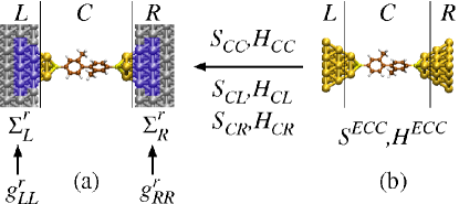
Figure 1: Quantum transport scheme. The conduction properties of an atomic-sized contact (a) shall be studied. For this purpose it is divided into a $C$ region and two semi-infinite $L$ and $R$ electrodes. Using a similar division as for the contact, information on the electronic structure of the $C$ region ($S_{CC}$, $H_{CC}$) as well as the $CL$ and $CR$ couplings ($S_{CL}$, $H_{CL}$ and $S_{CR}$, $H_{CR}$) is extracted from the ECC (b). In order to obtain the self-energies $\Sigma_{L}^{r}$ and $\Sigma_{R}^{r}$ (a), the remaining task is to determine the electrode surface Green’s functions $g_{LL}^{r}$ and $g_{RR}^{r}$. This procedure is described further below in the text.

The goal is to describe the whole atomic-sized contact [Fig. 1(a)] consistently, by treating the $L$, $C$, and $R$ regions with the same basis set and exchange-correlation functional. We obtain the parameters $S_{CC}$ and $H_{CC}$ as well as the couplings to the electrodes $S_{CX}$ and $H_{CX}$ with $X=L,R$ from the extended central system (ECC) [Fig. 1(b)], in which we include large parts of the tips of the metallic electrodes. The division of the ECC into the $L$, $C$, and $R$ regions is performed so that the $C$ region is identical to that in Fig. 1(a). The atoms in the $L$ and $R$ parts of the ECC [blue-shaded regions in Fig. 1(a)] correspond to that part of the electrodes that is assumed to couple to $C$. The partitioning or division of the ECC is commonly made somewhere in the middle of the metal tips, and we will also refer to it as ”cut”. The electrodes [$L$ and $R$ regions in Fig. 1(a)] are modeled as surfaces of semi-infinite crystals, described by the surface Green’s functions $g_{XX}^{r}$. They are constructed from bulk parameters, extracted from large metal clusters. Further below we discuss in detail, how this is accomplished.

In our approach, we assume the metal tips included in the ECC to be large enough to satisfy basically two criteria. First, all the charge transfer between the $L$ and $R$ electrodes and the $C$ part of the contact should be accounted for. This ensures the proper alignment of the electronic levels in $C$ with $E_{F}$. Second, most of the metal tips, especially the $L$ and $R$ parts of the ECC, should resemble bulk as closely as possible. In this way, we can evaluate the surface Green’s functions by using bulk parameters of an infinitely extended crystal. Owing to surface effects caused by the finite size of the ECC, this can be satisfied only approximately. The mismatch between the parameters in the $L$ and $R$ regions of the contact and the ECC will thus lead to spurious scattering at the $LC$ and $CR$ interfaces. In principle this resistance can be eliminated systematically by including more atoms in the metal tips of the ECC. On the other hand, if the resistance in the $C$ region is much larger than the spurious $LC$ and $CR$ interface resistances, they will have little influence on the results.

II.3.2 Electrodes

We extract bulk parameters describing perfect crystals from large metal clusters. The complete procedure, which aims at determining the surface Green’s functions $g_{XX}^{r}$ with $X=L,R$ is summarized in Fig. 2. In this work we study exclusively electrode materials with an fcc structure, of which Au and Al are examples.

In a first step [Fig. 2(a)] we construct spherical metal clusters, henceforth called “spheres”. They are made up of atoms at positions $\{\vec{R}_{j}|\vec{R}_{j}=\sum_{n=1}^{3}j_{n}\vec{a}_{n}\wedge|\vec{R}_{j}|\leq R^{sphere}\}$ with the standard fcc primitive lattice vectors $\vec{a}_{n}$ and the sphere radius $R^{sphere}$. Here, we will use the vector of integer indices $j=\left(j_{1},j_{2},j_{3}\right)$ to characterize the atomic position $\vec{R}_{j}$. We do not relax the spheres, but set the lattice constant $a_{0}$ to its experimental literature value.Ashcroft and Mermin (1976) Increasing the radius $R^{sphere}$ should make the electronic structure in the center resemble that of a crystal. From the clusters we extract the overlap and Hamiltonian between the central atom at position $0$ and the neighboring ones at position $j$ (including $j=0$). This yields the matrix elements $S_{j\alpha,0\beta}^{sphere}$ and $H_{j\alpha,0\beta}^{sphere}$, where $\alpha$ and $\beta$ stand for the basis functions of the atoms at $j$ and $0$. For reasons of brevity, we will often suppress the orbital indices. $S_{j0}^{sphere}$ and $H_{j0}^{sphere}$ are then matrices with appropriate dimensions.

The bulk parameters $S_{j0}$, $H_{j0}$ need to satisfy the symmetries of the fcc space-group [Fig. 2(b)]. While $S_{j0}^{sphere}$ depends only on the relative position of atoms, surface effects due to the finite size of the fcc clusters lead to deviations from the translational symmetry for $H_{j0}^{sphere}$. A rotation may still be necessary to arrive at parameters $S_{j0}^{\left(X\right)}$, $H_{j0}^{\left(X\right)}$, which are adapted to the orientation of the electrode $X=L,R$ [Fig. 2(c)]. Details on the symmetrization procedure and the transformation of crystal parameters under rotations are presented in App. B. The parameters $S_{j0}^{\left(X\right)}$, $H_{j0}^{\left(X\right)}$ are finally employed to construct the semi-infinite crystals and to obtain the surface Green’s function $g_{XX}^{r}$ [Fig. 2(d)]. Due to the finite range of the couplings $S_{CX}$, $H_{CX}$, we need to determine $g_{XX}^{r}$ for the first few surface layers only [blue-shaded regions in Fig. 1(a)]. We compute these with the help of the decimation technique of Ref. Guinea et al., 1983, which we have generalized to deal with the nonorthogonal basis sets.Pauly (2007) The parameters $S_{j0}$, $H_{j0}$ can be computed once for a given metal and can then be used in transport calculations with electrodes of various spatial orientations.

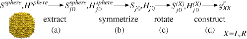
Figure 2: In order to obtain the electrode Green’s functions $g_{XX}^{r}$ for lead $X=L,R$, we determine bulk parameters from large metal clusters. In a first step (a) we extract overlap and hopping elements, $S_{j0}^{sphere}$, $H_{j0}^{sphere}$, from the cluster’s central atom to all its neighbors. They are (b) symmetrized by imposing the space-group of the electrode lattice. After (c) a rotation to adapt them to the orientation of the respective electrode, (d) $g_{XX}^{r}$ is constructed with the help of a decimation procedure.

For Au ($a_{0}=4.08$ Å) we have analyzed spheres ranging between 13 and 429 atoms, while for Al ($a_{0}=4.05$ Å) they vary between 13 and 555 atoms. Since we want to describe bulk, the parameters extracted from the largest clusters will obviously provide the best description. There is, however, an additional criterion, which necessitates the use of large metal clusters for a reliable description of the electrodes. As discussed in App. B.1, it is based on the positive-semidefiniteness of the bulk overlap matrix. We find a strong violation of this criterion, if the extraction of parameters is performed such that only the couplings of the cental atom to its nearest neighbors are considered. As a further demonstration of the quality of our description, we show in App. B.2 the convergence of the DOS with respect to $R^{sphere}$.

For the transport calculations we need a value for the Fermi energy. The biggest Au and Al spheres computed, Au₄₂₉ and Al₅₅₅, respectively, are very metallic. They exhibit differences between the highest occupied molecular orbital (HOMO) and the lowest unoccupied molecular orbital (LUMO) of less than $0.06$ eV. Therefore we set $E_{F}$ midway between these energies. In this way we obtain $E_{F}=-5.0$ eV for Au and $E_{F}=-4.3$ eV for Al. The values will be used in all the results below. Notice that the negative values of $E_{F}$ agree well with experimental work functions of $5.31$ to $5.47$ eV for Au and $4.06$ to $4.26$ eV for Al.Lide (1998)

III Metallic atomic contacts

In this chapter we explore the conduction properties of metallic atomic contacts of Au and Al. These systems, in particular atomic-sized Au contacts, have been studied in detail both experimentally and theoretically, and can therefore be used to test our method. We start by discussing the transport properties of the Au contacts, consisting of a four-atom chain, a three-atom chain, and a two-atom chain or “dimer”. Since Al does not form such chains, we consider only a single-atom contact. For all systems we analyze the transmission, its channel decomposition, and, in order to obtain knowledge about the conduction mechanism, the LDOS for atoms in the narrowest part of the contact. Moreover, we demonstrate the robustness of our transmission curves with respect to different partitionings of the large ECCs.

III.1 Gold contacts

Let us first discuss the electronic structure of Au, where we display the DOS in Fig. 3.

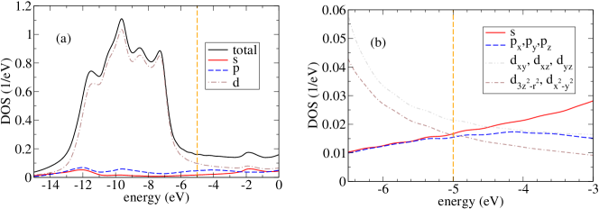
Figure 3: DOS for Au. (a) DOS resolved into $s$, $p$, and $d$ contributions and (b) DOS resolved into all individual orbital components. The dashed vertical line indicates $E_{F}=-5.0$ eV.

The Fermi energy at $E_{F}=-5.0$ eV is located in a fairly structureless, flat region somewhat above the $d$ band. Based on the electronic configuration [Xe].$4f^{14}.5d^{10}.6s^{1}$ of the atom, one might have expected a strong contribution only from the $s$ orbitals at $E_{F}$. But, as is visible from Fig. 3(b), $s$, $p$, and $d$ states all yield comparable contributions. This signifies that valence orbitals hybridize strongly in the metal.

When an atomic contact of Au is in a dimer or atomic chain configuration, a conductance of around $1G_{0}$ is expected from experimental measurementsScheer et al. (1998); Ludoph and van Ruitenbeek (2000); Yanson (2001); Yanson et al. (2005); Thijssen et al. (2006) as well as from theoretical studies.Cuevas et al. (1998); Brandbyge et al. (2002); Mozos et al. (2002); Lee et al. (2004); Dreher et al. (2005) The analysis shows that this value of the conductance is due to a single, almost fully transparent transmission channel. It arises dominantly from the $s$ orbitals of the noble metal Au, since the electronic structure in the narrowest part of the contact resembles more the electronic configuration of the atom.Scheer et al. (1998); Cuevas et al. (1998)

III.1.1 Determination of contact geometries

Despite the consensus that the conductance of atomic chains of Au is around $1G_{0}$, the precise atomic positions play an important role.Yanson et al. (1998); Dreher et al. (2005) Therefore it is necessary to construct reference geometries that have been studied with a well-established transport method. We choose to compare to results obtained with TRANSIESTA.Brandbyge et al. (2002) The ECCs investigated are shown in Fig. 4.

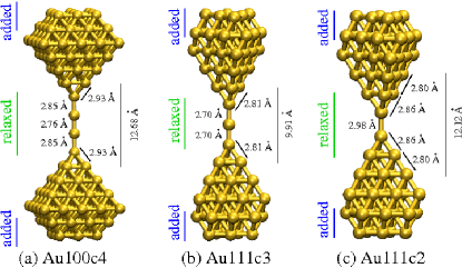
Figure 4: ECCs for Au. (a) Au100c4 is a four-atom Au chain, (b) Au111c3 is a three-atom Au chain, and (c) Au111c2 is a two-atom Au chain or dimer contact. For (a) electrodes are oriented in the [$100$] direction, while for (b) and (c) this is the [$111$] direction. The main crystallographic direction is assumed to be parallel to the $z$ axis. Indicated are also the most important bond distances together with information on the construction of the ECCs.

The four-atom Au chain with electrodes oriented in the [$100$] direction, called Au100c4, corresponds to a contact geometry examined in Ref. Frederiksen et al., 2004 [see Fig. 1(b) therein]. The three-atom Au chain, Au111c3, is similar to a configuration in Fig. 9(d) of Ref. Brandbyge et al., 2002. In addition, we study a Au dimer contact, Au111c2, where a two-atom chain is forming the narrowest part. In contrast to Au100c4, for the latter two contacts the electrodes are along the [$111$] direction.

Let us briefly explain, how we determine these geometries (Fig. 4). For Au100c4 we construct two ideal, atomically sharp Au [$100$] pyramids, with two atoms in between. The pyramids end with the layer consisting of 25 atoms. The distance between the layers containing four atoms is set to $12.68$ Å [Fig. 4(a)], as in Ref. Frederiksen et al., 2004. Next we relax the four chain atoms without imposing symmetries, keeping all other atoms fixed. After geometry optimization, we find that the configuration agrees well with symmetry $D_{4h}$. We add two more Au layers with 16 and 9 atoms on each side, where the ECC now consists of 162 atoms, and perform a final DFT calculation, exploiting the symmetry $D_{4h}$. As compared to Ref. Frederiksen et al., 2004, all bond distances indicated in Fig. 4(a) agree to within $0.01$ Å, except for the distance between the central chain atoms, where our distance is shorter by $0.07$ Å. For Au111c3 we proceed similarly to Au100c4 [Fig. 4(b)]. We start with two perfect Au [$111$] pyramids, set the distance between the Au layers with 3 atoms to $9.91$ Å,Brandbyge et al. (2002) and cut the pyramid off at the layers containing $10$ atoms. Then we add one atom in the middle, relax the three chain atoms, add two layers on each side with 12 and 6 atoms, and perform a calculation in symmetry $D_{3d}$. Au111c3 consists of 77 atoms in total. Our bond distances agree with those in Fig. 9(d) of Ref. Brandbyge et al., 2002 to within $0.02$ Å. For Au111c2 we include also the first Au layer in the geometry optimization process. The distance between the fixed layers with 6 atoms is $12.12$ Å. Otherwise the steps are the same as for Au111c3. The ECC is computed in symmetry $D_{3d}$ and consists of 76 atoms. In the parts excluded from the geometry optimization, atoms are all positioned on the bulk fcc lattice, where we set the lattice constant to the experimental value of $4.08$ Å, which corresponds to a nearest-neighbor distance of $2.88$ Å. In each ECC the main crystallographic direction is aligned with the $z$ axis, which is the transport direction.

III.1.2 Four-atom gold chain

Let us now study the conduction properties for the contact Au100c4 [Fig. 5(a)].

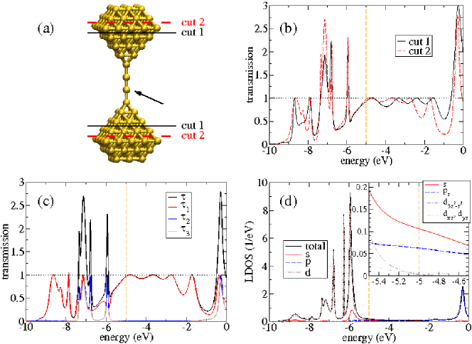
Figure 5: Au100c4. (a) ECC with two different partitionings into $L$, $C$, and $R$ regions, cuts 1 and 2, and (b) the transmission as a function of the energy for these cuts. For cut 2 (c) transmission resolved into its transmission channels and (d) LDOS of the chain atom indicated in (a).

There are different possibilities to partition the ECC into the $L$, $C$, and $R$ regions. The cuts should be done so that $L$ and $R$ are unconnected ($S_{LR}=0$ and $H_{LR}=0$, see Sec. II.2). Hence the $C$ region must be long enough. In order to describe well the coupling to the electrode surface (Fig. 1), it is furthermore necessary to have sufficiently many layers in the $L$ and $R$ regions. We observe that at least two layers are needed to obtain reasonable transmission curves. For the two different cuts of Fig. 5(a) $\tau(E)$ is plotted in Fig. 5(b). In both cases it is found to be almost identical, indicating a sufficient robustness of our method. The transmissions at the Fermi energy are $\tau(E_{F})=0.93$ and $0.98$ for cuts 1 and 2, respectively. These values correspond well to the result $\tau(E_{F})=0.99$ of Ref. Frederiksen et al., 2004.

For cut 2 it is visible in Fig. 5(c) that the transmission at $E_{F}$ is dominated by a single channel, in good agreement with experimental observationsScheer et al. (1998) and previous theoretical studies.Brandbyge et al. (2002); Mozos et al. (2002) In general, the electronic structure at the narrowest part should have the most decisive influence on the conductance of an atomic contact. Therefore we plot in Fig. 5(d) the LDOS of the atom indicated by the arrow in Fig. 5(a), resolved in its individual orbital contributions. Compared to the bulk DOS of Fig. 3, it is dominated by $s$ at $E_{F}$, where the contributions of all other orbitals than $s$ and $p_{z}$ are suppressed. These two orbitals will form the almost fully transparent transmission channel, which is radially symmetric with respect to the $z$ axis.

III.1.3 Three-atom gold chain

Exactly the same analysis will now be carried out for the contact Au111c3. In Fig. 6 the geometry of the ECC, the transmission for different partitionings, the transmission channels, and the LDOS of the central chain atom are shown.

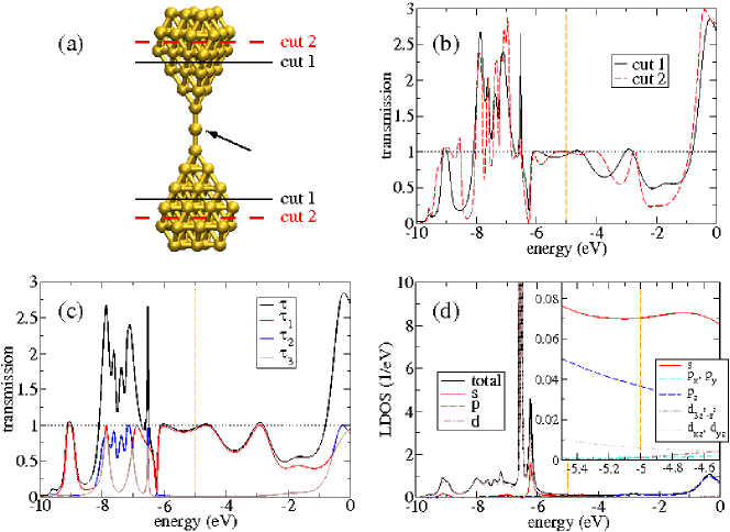
Figure 6: Au111c3. (a) ECC with two different partitionings into $L$, $C$, and $R$ regions, cuts 1 and 2, and (b) the transmission as a function of the energy for these cuts. For cut 1 (c) transmission resolved into its transmission channels and (d) LDOS of the central chain atom indicated in the ECC.

As for Au100c4, we observe that the different cuts yield very similar transmission curves [Fig. 6(b)]. Furthermore all the basic features in $\tau(E)$ are the same as in the TRANSIESTA calculation [see Fig. 11(d) of Ref. Brandbyge et al., 2002]. Above the $d$ band, which exhibits a very narrow and high final peak, there is a dip in $\tau(E)$ in both cases. The transmission recovers, however, and a flat region with a value of around one is visible. At the Fermi energy cuts 1 and 2 yield $\tau(E_{F})=0.96$ and $0.99$, respectively. This is in reasonable agreement with $\tau(E_{F})=0.94$ in Ref. Brandbyge et al., 2002, considering the differences in the electrode geometry, basis set, and exchange-correlation functional. We observe from Fig. 6(c) for cut 1 that the transmission at $E_{F}$ is dominated by a single transmission channel, and the LDOS indicates a dominant contribution of $s$ orbitals [Fig. 6(d)]. In addition, the peak structures in $\tau(E)$ for the $d$ states correspond well to peaks in the LDOS. This observation can also be made in Figs. 5(c) and 5(d) for Au100c4.

III.1.4 Two-atom gold chain

The transmission and LDOS resolved into transmission channels and orbital components, respectively, are shown in Fig. 7 for the dimer contact Au111c2.

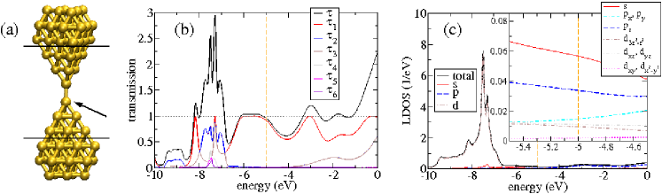
Figure 7: Au111c2. (a) ECC, and for the cut and atom indicated (b) the transmission resolved into its transmission channels and (c) the LDOS with its individual orbital contributions, respectively.

As for Au100c4 and Au111c3 we observe a single dominant channel at $E_{F}$, and $\tau(E_{F})=0.96$. The finding of such a dominant channel for chains of two or more atoms is in good agreement with our analysis of less symmetric contacts, which were based on a combination of a tight-binding model and classical molecular dynamics simulations.Dreher et al. (2005) However, that $\tau(E)$ increases partly even above one in the vicinity of $E_{F}$, signals that the influence of other channels is increased as compared to Au100c4 and Au111c3. Indeed, the LDOS of the atom in the narrowest part of the constriction [Figs. 7(a) and 7(c)] shows in particular increased $p_{x}$ and $p_{y}$ contributions. Also, the $d$ states exhibit a less pronounced peak structure than was visible in Figs. 5(d) and 6(d). This is due to the higher coordination number of the atom and the enhanced coupling to the electrodes.

III.2 Aluminum contacts

As is visible from the bulk DOS in Fig. 8, the electronic structure of Al differs substantially from that for Au.

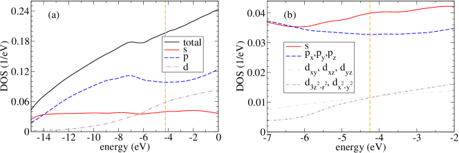
Figure 8: DOS for Al. (a) DOS resolved into $s$, $p$, and $d$ contributions and (b) DOS resolved into all individual orbital components. The dashed vertical line indicates $E_{F}=-4.3$ eV.

While the latter is a noble metal with an $s$ valence, the Al atom has the electronic configuration [Ne].$3s^{2}.3p^{1}$ with an open $p$ shell, and the metal is hence considered $sp$-valent. The strong contribution of $s$ and $p$ states is also observed in the DOS, where $d$ states play only a minor role. As compared to Au, the DOS exhibits a noticeable energy dependence around $E_{F}$.

For Al we study an ideal fcc [$111$] pyramid, consisting of 251 atoms [Fig. 9(a)], henceforth referred to as Al111c1. Ideal means that the atoms are positioned on an fcc lattice with the experimental lattice constant $a_{0}=4.05$ Å. We have already reported results for Al dimer contacts in Ref. Wohlthat et al., 2007.

III.2.1 Aluminum single-atom contact

In Fig. 9 the transmission is displayed for three different partitionings of the ECC Al111c1.

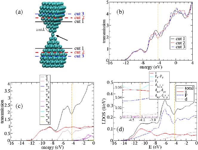
Figure 9: Al111c1. (a) ECC with three different partitionings into $L$, $C$, and $R$ regions, cuts 1, 2, and 3, and (b) the transmission as a function of the energy for these cuts. For cut 2 (c) the transmission resolved into its transmission channels and (d) the LDOS of the central atom, indicated by the arrow in (a). The nearest-neighbor distance shown in the ECC is identical for all atoms.

Also shown are the transmission channels and the LDOS of the atom in the narrowest part of the contact for a selected cut. For energies below $-6$ eV, there are practically no differences visible between the curves for the three different partitionings. Nevertheless, some deviations arise at $E_{F}$, and we obtain $\tau(E_{F})=2.36$ (cut 1), $1.88$ (cut 2), and $2.23$ (cut 3). Similar to Au, we attribute these 20% relative variations to spurious scattering at the $LC$ and $CR$ interfaces. Our values for $\tau(E_{F})$ of around two agrees nicely with those reported for single-atom contacts in Ref. Jelínek et al., 2003. Compared to Au, the transmission-channel structure has changed in an obvious way. There are three channels at $E_{F}$, which is in line with experimental observations of Refs. Scheer et al., 1997, 1998. Due to the $D_{3d}$ symmetry of the ECC, transmission-channel degeneracies arise, where in particular $\tau_{2}=\tau_{3}$. As is visible from the LDOS, these additional channel contributions mainly stem from the $p_{x}$ and $p_{y}$ orbitals, while $s$ and $p_{z}$ are forming the nondegenerate $\tau_{1}$.Scheer et al. (1998); Cuevas et al. (1998); Pauly et al. (2006)

IV Conclusions

We have developed a cluster-based method to study the charge transport properties of molecular and atomic contacts. We treat the electronic structure at the level of DFT, and describe transport in terms of the Landauer formalism expressed with standard Green’s function techniques. Special emphasis is placed on the modeling of the electrodes and the construction of the associated bulk parameters from spherical metal clusters. We showed that these clusters need to be sufficiently large to produce reliable bulk parameters, where a criterion for the extent of the spherical clusters is set by the overlap of the nonorthogonal basis functions. In our studies we crucially rely on the accurate and efficient quantum-chemical treatment of systems consisting of several hundred atoms, made possible by use of the quantum chemistry package TURBOMOLE. Compared to supercell approached, our method has the advantage that we genuinely describe single-atom or single-molecule contacts.

As an application of our method we analyzed Au and Al atomic contacts. Studying a four-, a three-, and a two-atom chain with varied electrode lattice orientations for Au, we found a conductance close to $1G_{0}$, carried by a single transmission channel. Next we investigated an ideal Al single-atom contact, and found three transmission channels to contribute significantly to the conductance of around $2G_{0}$. These results are in good agreement with previous experimental and theoretical investigations. Both for Au and Al we demonstrated the robustness of our transmission curves with respect to partitionings of the contact systems. The results illustrate the applicability of our method to various electrode materials.

Beside the metallic atomic contacts examined here, the presented method has been applied in the field of molecular electronics. Studies include the dc conduction properties of dithiolated-oligophenylene and diamino-alkane junctionsViljas et al. (2007); Pauly et al. (2008, ); Wohlthat et al. (2008) as well as oxygen adsorbates in Al contacts.Wohlthat et al. (2007) In addition, the thermopowerPauly et al. and photoconductanceViljas et al. (2007) of molecular junctions has been investigated in this way. Our studies demonstrate the value of parameter-free modeling for understanding transport at the molecular and atomic scale.

Appendix A Nonorthogonal basis sets

For practical reasons one often employs nonorthogonal basis sets in quantum-chemical calculations, consisting for example of a finite set of Gaussian functions. The electronic structure is described in the spirit of the linear combination of atomic orbitals (LCAO),Szabo and Ostlund (1996); Koch and Holthausen (2001); Atkins and Friedman (2005) and this is also how TURBOMOLE is implemented. While it is in principle always possible to transform to an orthogonal basis, it may be more convenient to work directly with the nonorthogonal states.

A concise mathematical description using nonorthogonal basis states can be formulated in terms of tensors. The formalism is presented in a fairly general form in Ref. Artacho and del Bosch, 1991, where also the modifications of second quantization are addressed. Below we discuss some of the subtleties related to the use of nonorthogonal basis functions that are important for our method.Pauly (2007) Since the basis functions are real-valued in our case, the full complexity of the tensor formalism is not needed.Iben (1999); Borisenko and Tarapov (1979) Furthermore we use a simplified notation, where all tensor indices appear as subscripts of matrices.

A.1 Current formula for nonorthogonal, local basis sets

The most important quantity for transport calculations is the electric current. In the NEGF formalism, its determination requires a separation of the contact into subsystems similar to Fig. 1(a).Caroli et al. (1971); Meir and Wingreen (1992); Datta (2005) However, due to the overlap of the basis functions in a nonorthogonal basis, the charges of the subsystems are not well defined. Different ways of determining them exist, e.g. the Mulliken or Löwdin population analysis.Szabo and Ostlund (1996) Despite these additional complications, the Landauer formula [Eq. (2)] can be derived in a similar fashion as for an orthogonal basis. Recent discussions of the derivation can be found in Refs. Viljas et al., 2005; Thygesen, 2006.

A.2 Single-particle Green’s functions

Consider the single-particle Hamiltonian $H$ describing the entire system. The retarded Green’s operator is defined as $G^{r}(E)=\left[\left(E+i0^{+}\right)\mathbbm{1}-H\right]^{-1}$. Now consider the local, nonorthogonal basis $|i\rangle$ with the (covariant) matrix elements of the overlap $S_{ij}=\left\langle i\right.\left|j\right\rangle$ and the Hamiltonian $H_{ij}=\left\langle i\right|H\left|j\right\rangle$.Iben (1999); Borisenko and Tarapov (1979) Compared to Sec. II.2 the index $i$, used throughout this appendix, is a collective index, denoting both the position at which the basis state is centered and its type. The components of the retarded Green’s function, defined by $G^{r}=\sum_{i,j}|i\rangle G_{ij}^{r}\langle j|$, satisfy the equationXue et al. (2002)

$$\sum_{k}\left[\left(E+i0^{+}\right)S_{jk}-H_{jk}\right]G_{kl}^{r}(E)=\delta_{jl}.$$ (12)

The Green’s function $G_{CC}^{r}$ is defined as $G_{ij}^{r}$ restricted to the central region $C$. It can be calculated according to Eq. (5). Due to the nonorthogonal basis, the perturbation that couples $C$ to the lead $X=L,R$ and enters the self-energy [Eq. (6)], is given by $H_{CX}-ES_{CX}$ and thus includes also an overlap contribution. It is interesting to observe that as $E\rightarrow\infty$ the self-energies and the Green’s function behave as

$$\Sigma_{X}^{r}(E) \underrightarrow{E\rightarrow\infty} ES_{CX}\left(S_{XX}\right)^{-1}S_{XC}$$ (13)

$$G_{CC} \underrightarrow{E\rightarrow\infty} E^{-1}\left(S^{-1}\right)_{CC}$$ (14)

with

$$\left(S^{-1}\right)_{CC}=\left[S_{CC}+\sum_{X=L,R}S_{CX}\left(S_{XX}\right)^{-1}S_{XC}\right]^{-1}.$$ (15)

Thus also the inverse overlap matrix of $C$ is “renormalized” due to the coupling to the leads.

A.3 Local density of states

Using a set of orthonormal energy eigenstates $\left|\mu\right\rangle$ that satisfy $H\left|\mu\right\rangle=\varepsilon_{\mu}\left|\mu\right\rangle$, we obtain the decomposition $\rho_{\mu\nu}(E)=\langle\mu|\rho(E)|\nu\rangle=\sum_{\mu}\delta(E-\varepsilon_{\mu})\delta_{\mu\nu}$ of the spectral density defined by Eq. (9). Clearly $\rho_{\mu\nu}(E)$ fulfills the normalization

$$\int_{-\infty}^{\infty}dE\rho_{\mu\nu}(E)=\delta_{\mu\nu}.$$ (16)

If, instead, we consider the components defined by $\rho_{ij}(E)=-\mathrm{Im}\left[G_{ij}^{r}(E)\right]/\pi$, where $G_{ij}^{r}(E)$ is given by Eq. (12), we find

$$\int_{-\infty}^{\infty}dE\rho_{ij}(E)=\left(S^{-1}\right)_{ij}.$$ (17)

The normalization of Eq. (16) can be recovered by performing a Löwdin orthogonalization of the basis

$$\int_{-\infty}^{\infty}dE(S^{1/2})_{ik}\rho_{kl}(E)(S^{1/2})_{lj}=\delta_{ij}$$ (18)

Let us analyze the LDOS of the central region $\rho_{CC}(E)=-\mathrm{Im}\left[G_{CC}^{r}(E)\right]/\pi$, which is $\rho_{ij}(E)$ restricted to $C$. Analogously to Eq. (18), we have defined the LDOS at atom $i$ and its decomposition into orbitals $\alpha$ in Eqs. (10) and (11). Since $\rho_{CC}(E)$ is a positive-semidefinite matrix, it is easy to show that $\mathrm{LDOS}_{i\alpha}(E)$ is positive for all $E$. However, the normalization $\int_{-\infty}^{\infty}dE\mathrm{LDOS}_{i\alpha}(E)=1$ is only approximately fulfilled. This could be corrected by multiplying in Eq. (11) with $\left(S^{-1}\right)_{CC}^{-1/2}$ [Eq. (15)] instead of $S_{CC}^{1/2}$. But since the self-energy contributions $\sum_{X=L,R}S_{CX}\left(S_{XX}\right)^{-1}S_{XC}$ constitute only a surface correction, their neglect may be justified for atoms in the middle of $C$.

Appendix B Description of electrodes

B.1 Size requirement for the cluster construction

How large do the spherical metal clusters, involved in the construction in Fig. 2, need to be for a convergence of the bulk parameters? Since the matrix elements of the Hamiltonian and the overlap decay similarly with increasing interatomic distance, we can concentrate on the overlap. For it a rather well-defined criterion can be found: The clusters should so large that the extracted bulk overlap matrix is positive-semidefinite.

We define states $\left|\vec{k},\alpha\right\rangle=\sum_{j}e^{i\vec{k}\cdot\vec{R}_{j}}\left|j,\alpha\right\rangle$ in $k$-space. Since $S_{i\alpha,j\beta}=\left\langle i,\alpha\right.\left|j,\beta\right\rangle$ is a positive-semidefinite matrix,Szabo and Ostlund (1996) the same is true for the overlap in $k$-space

$$S_{\alpha\beta}(\vec{k},\vec{k}^{\prime})=\left\langle\vec{k},\alpha\right.\left|\vec{k}^{\prime},\beta\right\rangle = \sum_{l,m}e^{-i\vec{k}\cdot\vec{R}_{l}}S_{l\alpha,m\beta}e^{i\vec{k}\cdot\vec{R}_{m}}$$

$$= N\delta_{\vec{k},\vec{k}^{\prime}}S_{\alpha\beta}(\vec{k}),$$

where we used that $S_{l\alpha,m\beta}=S_{\left(l-m\right)\alpha,0\beta}$. In the expression, $N$ is the number of atoms in the crystal and

$$S_{\alpha\beta}(\vec{k})=\sum_{j}e^{-i\vec{k}\cdot\vec{R}_{j}}S_{j\alpha,0\beta}.$$ (20)

In order to study the positive-semidefiniteness of $S_{\alpha\beta}(\vec{k},\vec{k}^{\prime})$ it is hence sufficient to investigate the behavior of $S_{\alpha\beta}(\vec{k})$. To do so for a complex quantum-chemistry basis set, we define the positive-definiteness measure

$$\xi(R^{sphere})=\min_{\vec{k}}(\mathcal{S}(\vec{k})).$$ (21)

In this expression $\mathcal{S}(\vec{k})$ is the smallest eigenvalue of the matrix $S_{\alpha\beta}(\vec{k})$, where $S_{\alpha\beta}(\vec{k})$ is constructed from the crystal parameters extracted from a cluster with radius $R^{sphere}$ [$S_{\alpha\beta}(\vec{k})=\sum_{\vec{R}_{j};|\vec{R_{j}}|\leq R^{sphere}}e^{-i\vec{k}\cdot\vec{R}_{j}}S_{j\alpha,0\beta}$]. In the discrete Fourier transformations we assume periodic boundary conditions with a finite periodicity length along the standard primitive lattice vectors.Ashcroft and Mermin (1976); Pauly (2007) $R^{sphere}$ must be chosen large enough for $\xi$ to be positive or, if $\xi$ remains negative, it must at least be sufficiently small in absolute value.

Let us first illustrate the behavior of $\xi$ at the example of an $s$-orbital model. Gaussian $s$ functions are described by

$$\phi_{s}(\vec{r})=\left(\frac{2\alpha}{\pi}\right)^{3/4}e^{-\alpha\left|\vec{r}\right|^{2}}$$ (22)

with an exponent $\alpha$, characterizing the radial decay. Hence, the overlap between two atoms

$$S_{js,0s}=\int d^{3}r\phi_{s}(\vec{r}-\vec{R}_{j})\phi_{s}(\vec{r})=e^{-\alpha R_{j}^{2}/2}$$ (23)

decays with their distance $R_{j}=|\vec{R}_{j}|$ like a Gaussian function. We consider an infinitely extended chain with atoms at equally spaced positions along the $x$-axis ($\vec{R}_{j}=j_{1}a_{0}\vec{e}_{x}$). The overlap from a selected atom to its neighbors drops off exponentially as shown in Fig. 10(a).

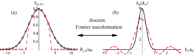
Figure 10: $s$-orbital-chain model. (a) The overlap $S_{js,0s}$ of an atom with its neighbors at positions $R_{j,x}=j_{1}a_{0}$ with $j_{1}=0,\pm 1,\ldots$. (b) Overlap $S_{ss}(k_{x})$ after a discrete Fourier transformation. In both cases the solid line is for a large and the dashed line for a small cluster.

The Fourier transformation will again result in a Gaussian with purely positive values $S_{ss}(k_{x})$ [Fig. 10(b)]. If, however, overlap matrix elements are taken into account only up to a certain maximum value $|\vec{R}_{j}|\leq R^{sphere}$, as in a finite cluster, a rough $\sin(k_{x})/k_{x}$-behavior results, where $S_{ss}(k_{x})$ becomes negative at certain $k$-values. Upon an increase of $R^{sphere}$, $S_{ss}(k_{x})$ will evolve into a Gaussian function and $\xi$ will thus approach zero from below. The negative tails of $S_{ss}(k_{x})$ are unphysical, and our observation implies that the clusters used to extract bulk parameters (Fig. 2) need to be of a sufficiently large radius $R^{sphere}$, in order to obtain a reliable description of a crystal. Obviously, the magnitude of $R^{sphere}$ depends on the basis set chosen.

Figure 11: The positive-definiteness measure $\xi$ for Au and Al as a function of $R^{sphere}$. Beside the SVP basis set, the behavior of $\xi$ is also shown for LANL2DZ, used in Refs. Damle et al., 2001, 2002. $S(\vec{k})$ [Eq. (20)] is evaluated at $32^{3}$ $k$-points. The radius $R^{sphere}$ has been scaled with the respective lattice constants ($a_{0}=4.08$ Å for Au and $a_{0}=4.05$ Å for Al).

In Fig. 11 we plot the behavior of $\xi$ as a function of $R^{sphere}$ for Au and Al. Beside the results for the SVP basis set, we display $\xi$ for Au also for the basis set LANL2DZ, used in Refs. Damle et al., 2001, 2002. It is visible that $\xi$ is positive for a single atom ($R^{sphere}=0$), but negative for small spheres. With increasing $R^{sphere}$, $\xi$ approaches $0$ from below similar to the $s$-orbital model. We find that the elimination of diffuse functions reduces the radius $R^{sphere}$ for $\xi$ to become positive or negligibly small. For practical reasons it may happen that $R^{sphere}$ cannot be chosen large enough to fulfill the positive-semidefiniteness criterion $\xi\geq 0$. In such a case negative eigenvalues of $S_{\alpha\beta}(\vec{k})$ can lead to negative eigenvalues of the scattering-rate matrices $\Gamma_{X}$ [Eq. (7)], since $\rho_{XX}=-\mathrm{Im}\left[g_{XX}^{r}\right]/\pi$ may no longer be positive-semidefinite (see also the discussion in Sec. A.3).

B.2 Bulk densities of states

The DOS can be used as another measure for the convergence to a solid-state description. With a $k$-space Hamiltonian in an orthogonal basis set $H^{orth}(\vec{k})$, it is given as

$$\mathrm{DOS}(E)=\sum_{\alpha}\mathrm{DOS}_{\alpha}(E)=-\frac{1}{\pi}\mathrm{Tr}_{\alpha}\left[\mathrm{Im}\left[G_{0\alpha,0\alpha}^{orth,r}(E)\right]\right],$$ (24)

where $\alpha$ runs over all basis functions on a bulk atom and $G_{00}^{orth,r}(E)=\int_{BZ}d^{3}kG^{orth,r}(\vec{k},E)/V_{BZ}$ with $G^{orth,r}(\vec{k},E)=\left[E\mathbbm{1}-H^{orth}(\vec{k})\right]^{-1}$ and with the volume $V_{BZ}$ of the first Brillouin zone $BZ$. The orthogonal Hamiltonian can be obtained in several ways. Two possible choices are (i) to Fourier transform $S_{j0}$ and $H_{j0}$ and perform a Löwdin orthogonalization in $k$-space $H^{orth}(\vec{k})=S^{-1/2}(\vec{k})H(\vec{k})S^{-1/2}(\vec{k})$ or (ii) to construct $H_{j0}^{orth}$, which involves the Löwdin transformation $H^{sphere,orth}=\left(S^{-1/2}\right)^{sphere}H^{sphere}\left(S^{-1/2}\right)^{sphere}$ in real space, extraction of $H_{j0}^{sphere,orth}$ and the imposing of the fcc space group, and to carry out the Fourier transformation only thereafter. For parameters extracted from large enough clusters we observe the equivalence of the DOS construction with respect to the two different orthogonal Hamiltonians $H^{orth}(\vec{k})$. If $\xi$ remains (slightly) negative due to a too small $R^{sphere}$, then the construction of the DOS from $H_{j0}^{orth}$ [procedure (ii)] is of a higher quality than that resulting from the Löwdin orthogonalization in $k$-space [procedure (i)].

In Fig. 12 we show the DOS as constructed via procedure (ii) with parameters extracted from different Au and Al spheres with 141 to 555 atoms.

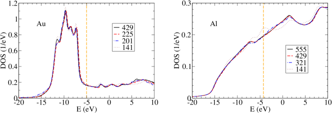
Figure 12: DOS of Au and Al constructed from parameters extracted from fcc spheres with atom numbers between 141 and 555. The vertical dashed line indicates the Fermi energy $E_{F}$.

We observe that the DOS seems well converged with respect to $R^{sphere}$ both for Au and Al for the largest spherical clusters Au₄₂₉ and Al₅₅₅.

B.3 Transformation of electrode parameters under rotations

We assume that two coordinate systems are connected by the rotation $\varrho$, where $\vec{r}^{\prime}=\varrho\vec{r}$. The transformation properties of the electrode parameters

$$Y_{j\alpha,0\beta}=\left\langle j,\alpha\right|Y\left|0,\beta\right\rangle=\int d^{3}r\phi_{\alpha}(\vec{r}-\vec{R}_{j})Y(\vec{r})\phi_{\beta}(\vec{r})$$

with $Y=S,H$ are determined by those of the basis functions $\left\langle\vec{r}\left.\right|j,\alpha\right\rangle=\phi_{\alpha}(\vec{r}-\vec{R}_{j})$. The Gaussian basis functions used by TURBOMOLE are characterized by the angular momentum $l$ and the multiplicity $\nu=1,\ldots,2l+1$, and $\alpha$ is a collective index for both. The rotated basis functions of angular momentum $l$ can be expressed asHamermesh (1989)

$$\left[\psi^{\prime}\right]_{\nu}^{l}(\vec{r})=\psi_{\nu}^{l}(\varrho^{-1}\vec{r})=\sum_{\mu=1}^{2l+1}\psi_{\mu}^{l}(\vec{r})D_{\mu\nu}^{l}(\varrho)$$

with the representation $D_{\mu\nu}^{l}(\varrho)$ of the rotation $\varrho$. Using $Y^{\prime}(\vec{r})=Y(\varrho^{-1}\vec{r})$, it can be shown that the electrode parameters of the two coordinate systems are related by

$$Y_{\vec{R}_{j}\alpha,\vec{0}\beta}=\sum_{\mu,\nu}\left[D^{T}(\varrho)\right]_{\alpha\mu}Y^{\prime}_{\varrho\vec{R}_{j}\mu,\vec{0}\nu}D(\varrho)_{\nu\beta},$$ (25)

where $D(\varrho)$ is the representation of $\varrho$ in the employed basis set. By knowledge of the $D_{\mu\nu}^{l}(\varrho)$, $D(\varrho)$ can be constructed by the process of the addition of representations.Hamermesh (1989) If there are $n_{l}$ basis functions of angular momentum $l$ in the basis set describing $Y_{j\alpha,0\beta}$, we have

$$D(\varrho)=\oplus_{l}n_{l}D^{l}(\varrho),$$ (26)

where $\oplus$ denotes a direct sum.

Let us now give the explicit formulas for the $D^{l}(\varrho)$. In this work only $s$, $p$, and $d$ basis functions are used, and hence we restrict ourselves to $l=0$, $1$, and $2$. Since $s$ functions just depend on the radius, $\psi^{0}(\vec{r})=\psi^{0}(r)$, we have

$$D^{0}(\varrho)=1.$$ (27)

For $l=1$ there are three $p$ functions, $p_{1}=p_{x}=f_{1}(r)x$, $p_{2}=p_{y}=f_{1}(r)y$, and $p_{3}=p_{z}=f_{1}(r)z$, with a certain radial dependence $f_{1}(r)$.Atkins and Friedman (2005) Exploiting $\varrho^{-1}=\varrho^{T}$, we obtain $p^{\prime}_{i}=\sum_{j=1}^{3}p_{j}\varrho_{ji}$. Thus the $3\times 3$ representation of the rotation $\varrho$ for the $p$ functions is

$$D^{1}(\varrho)=\varrho=\left(\begin{array}[]{ccc}\varrho_{xx}&\varrho_{xy}&\varrho_{xz}\\ \varrho_{yx}&\varrho_{yy}&\varrho_{yz}\\ \varrho_{zx}&\varrho_{zy}&\varrho_{zz}\end{array}\right).$$ (28)

For $l=2$ there are five $d$ functions, where $d_{1}=d_{3z^{2}-r^{2}}=f_{2}(r)\left(3z^{2}-r^{2}\right)/\left(2\sqrt{3}\right)$, $d_{2}=d_{xz}=f_{2}(r)xz$, $d_{3}=d_{yz}=f_{2}(r)yz$, $d_{4}=d_{xy}=f_{2}(r)xy$, and $d_{5}=d_{x^{2}-y^{2}}=f_{2}(r)\left(x^{2}-y^{2}\right)/2$ with some radial dependence $f_{2}(r)$. The transformed $d$ functions are given as $d_{i}^{\prime}=\sum_{j=1}^{3}d_{j}\left[D^{2}\left(\varrho\right)\right]_{ji}$ with the $5\times 5$ representation

$$D^{2}(\varrho)=\left(\begin{array}[]{ccccc}\left(3\varrho_{zz}^{2}-1\right)/2&\sqrt{3}\varrho_{zx}\varrho_{zz}&\sqrt{3}\varrho_{zy}\varrho_{zz}&\sqrt{3}\varrho_{zx}\varrho_{zy}&\sqrt{3}\left(\varrho_{zx}^{2}-\varrho_{zy}^{2}\right)/2\\ \sqrt{3}\varrho_{xz}\varrho_{zz}&\varrho_{xx}\varrho_{zz}+\varrho_{zx}\varrho_{xz}&\varrho_{xy}\varrho_{zz}+\varrho_{xz}\varrho_{zy}&\varrho_{xx}\varrho_{zy}+\varrho_{xy}\varrho_{zx}&\varrho_{xx}\varrho_{zx}-\varrho_{xy}\varrho_{zy}\\ \sqrt{3}\varrho_{yz}\varrho_{zz}&\varrho_{yx}\varrho_{zz}+\varrho_{zx}\varrho_{yz}&\varrho_{yy}\varrho_{zz}+\varrho_{yz}\varrho_{zy}&\varrho_{yx}\varrho_{zy}+\varrho_{yy}\varrho_{zx}&\varrho_{yx}\varrho_{zx}-\varrho_{yy}\varrho_{zy}\\ \sqrt{3}\varrho_{xz}\varrho_{yz}&\varrho_{xx}\varrho_{yz}+\varrho_{yx}\varrho_{xz}&\varrho_{xy}\varrho_{yz}+\varrho_{yy}\varrho_{xz}&\varrho_{xx}\varrho_{yy}+\varrho_{xy}\varrho_{yx}&\varrho_{xx}\varrho_{yx}-\varrho_{xy}\varrho_{yy}\\ \sqrt{3}\left(\varrho_{xz}^{2}-\varrho_{yz}^{2}\right)/2&\varrho_{xx}\varrho_{xz}-\varrho_{yx}\varrho_{yz}&\varrho_{xy}\varrho_{xz}-\varrho_{yy}\varrho_{yz}&\varrho_{xx}\varrho_{xy}-\varrho_{yx}\varrho_{yy}&\left(\varrho_{xx}^{2}+\varrho_{yy}^{2}-\varrho_{xy}^{2}-\varrho_{yx}^{2}\right)/2\end{array}\right).$$ (29)

B.4 Imposing the fcc space-group

In this section we consider how to impose the fcc space-group on the parameters $H_{j\alpha,0\beta}^{sphere}$, extracted from the finite spherical fcc clusters [Fig. 2]. Assuming basis functions to be real-valued, the matrix elements of a translationally invariant Hamiltonian $H^{trans}$ are symmetric and obey the relations

$$H_{i\alpha,j\beta}^{trans}=H_{\left(i-j\right)\alpha,0\beta}^{trans}=H_{0\alpha,-\left(i-j\right)\beta}^{trans}=H_{-\left(i-j\right)\beta,0\alpha}^{trans}.$$ (30)

Owing to surface effects, the translational symmetry is not fulfilled by the parameters $H_{j\alpha,0\beta}^{sphere}$, as illustrated in Fig. 13.

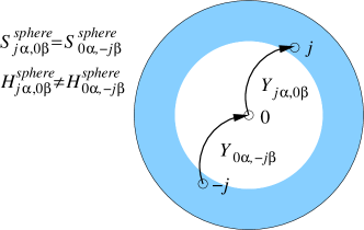
Figure 13: Necessity to impose the translational symmetry on the hopping elements $H_{j\alpha,0\beta}^{sphere}$. A finite spherical cluster is displayed. In blue-shaded areas surface effects are important. While the overlap elements $S_{j\alpha,0\beta}^{sphere}$ are translationally symmetric, this is not the case for $H_{j\alpha,0\beta}^{sphere}$. In particular $S_{j\alpha,0\beta}^{sphere}=S_{0\alpha,-j\beta}^{sphere}$, while $H_{j\alpha,0\beta}^{sphere}\neq H_{0\alpha,-j\beta}^{sphere}$ as illustrated in the plot, where $Y=S,H$.

Hence, although the deviations decrease with growing radius of the spheres, the translational symmetry needs to be enforced in order to describe a crystal. To avoid numerical errors, we impose at the same time the point-group symmetry $O_{h}$ although that symmetry is already present due to the shape of our clusters. Concerning the notation, we will call the parameters conforming to the $O_{h}$ point-group, the translational symmetry, and the fcc space-group $H_{j\alpha,0\beta}^{O_{h}}$, $H_{j\alpha,0\beta}^{trans}$, and $H_{j\alpha,0\beta}=H_{j\alpha,0\beta}^{fcc}$, respectively. We do not need to consider the overlap, since it depends only on the relative position of two atoms.

$O_{h}$ point-group symmetry

With Eq. (25) a Hamiltonian $H_{j\alpha,0\beta}^{O_{h}}$ conforming to the point-group symmetry can be constructed by averaging, for a given element of $H_{j\alpha,0\beta}^{O_{h}}$, over all $H_{j\alpha,0\beta}^{sphere}$ related to it by symmetry

$$H_{\vec{R}_{j}\alpha,\vec{0}\beta}^{O_{h}}=\frac{1}{N_{O_{h}}}\sum_{\varrho\in O_{h}}\sum_{\mu,\nu}\left[D^{T}(\varrho)\right]_{\alpha,\mu}H_{\varrho\vec{R_{j}}\mu,\vec{0}\nu}^{sphere}D(\varrho)_{\nu\beta}.$$ (31)

Here, $\varrho$ runs over all $N_{O_{h}}=48$ symmetry elements of the point group $O_{h}$.Hamermesh (1989); Corso (Springer, Berlin, 1996)

Translational symmetry

Using Eq. (30), the translational symmetry can be imposed by setting

$$H_{j\alpha,0\beta}^{trans}=\frac{1}{2}\left(H_{j\alpha,0\beta}^{sphere}+H_{-j\beta,0\alpha}^{sphere}\right).$$ (32)

Fcc space-group

The combined action of the $O_{h}$ point-group and the translational symmetry leads to the fcc space-group symmetry. With Eqs. (31) and (32) we obtain the fcc space-group symmetric parameters $H_{j\alpha,0\beta}=H_{j\alpha,0\beta}^{fcc}$ according to the prescription

$$H_{\vec{R_{j}}\alpha,\vec{0}\beta}^{fcc}=\frac{1}{2N_{O_{h}}}\sum_{\varrho\in O_{h}}\sum_{\mu,\nu}\left\{\left[D^{T}\left(\varrho\right)\right]_{\alpha\mu}H_{\varrho\vec{R_{j}}\mu,\vec{0}\nu}^{sphere}D\left(\varrho\right)_{\nu\beta}+\left[D^{T}\left(\varrho\right)\right]_{\beta\mu}H_{-\varrho\vec{R_{j}}\mu,\vec{0}\nu}^{sphere}D\left(\varrho\right)_{\nu\alpha}\right\}.$$ (33)

References

- Nitzan and Ratner (2003) A. Nitzan and M. A. Ratner, Science 300, 1384 (2003).
- Nazin et al. (2003) G. V. Nazin, X. H. Qiu, and W. Ho, Science 302, 77 (2003).
- Tao (2006) N. J. Tao, Nature Nanotechnology 1, 173 (2006).
- Lindsay and Ratner (2007) S. M. Lindsay and M. A. Ratner, Adv. Mater. 19, 23 (2007).
- Akkerman and de Boer (2008) H. B. Akkerman and B. de Boer, J. Phys.: Condens. Matter 20, 013001 (2008).
- Agraït et al. (2003) N. Agraït, A. L. Yeyati, and J. M. van Ruitenbeek, Phys. Rep. 377, 81 (2003).
- Brandbyge et al. (2002) M. Brandbyge, J.-L. Mozos, P. Ordejón, J. Taylor, and K. Stokbro, Phys. Rev. B 65, 165401 (2002).
- Palacios et al. (2002) J. J. Palacios, A. J. Pérez-Jiménez, E. Louis, E. San-Fabián, and J. A. Vergés, Phys. Rev. B 66, 035322 (2002).
- Xue et al. (2001) Y. Xue, S. Datta, and M. A. Ratner, J. Chem. Phys. 115, 4292 (2001).
- Taylor et al. (2001) J. Taylor, H. Guo, and J. Wang, Phys. Rev. B 63, 245407 (2001).
- Fujimoto and Hirose (2003) Y. Fujimoto and K. Hirose, Phys. Rev. B 67, 195315 (2003).
- Jelínek et al. (2003) P. Jelínek, R. Pérez, J. Ortega, and F. Flores, Phys. Rev. B 68, 085403 (2003).
- Havu et al. (2004) P. Havu, V. Havu, M. J. Puska, and R. M. Nieminen, Phys. Rev. B 69, 115325 (2004).
- Tada et al. (2004) T. Tada, M. Kondo, and K. Yoshizawa, J. Chem. Phys. 121, 8050 (2004).
- Thygesen and Jacobsen (2005) K. S. Thygesen and K. W. Jacobsen, Chem. Phys. 319, 111 (2005).
- Damle et al. (2001) P. S. Damle, A. W. Gosh, and S. Datta, Phys. Rev. B 64, 201403 (2001).
- Wortmann et al. (2002) D. Wortmann, H. Ishida, and S. Blügel, Phys. Rev. B 65, 165103 (2002).
- Evers et al. (2004) F. Evers, F. Weigend, and M. Koentopp, Phys. Rev. B 69, 235411 (2004).
- Khomyakov and Brocks (2004) P. A. Khomyakov and G. Brocks, Phys. Rev. B 70, 195402 (2004).
- Calzolari et al. (2004) A. Calzolari, N. Marzari, I. Souza, and M. Buongiorno Nardelli, Phys. Rev. B 69, 035108 (2004).
- Heurich et al. (2002) J. Heurich, J. C. Cuevas, W. Wenzel, and G. Schön, Phys. Rev. Lett. 88, 256803 (2002).
- Rocha et al. (2006) A. R. Rocha, V. M. García-Suárez, S. Bailey, C. Lambert, J. Ferrer, and S. Sanvito, Phys. Rev. B 73, 085414 (2006).
- Ferretti et al. (2005) A. Ferretti, A. Calzolari, R. Di Felice, F. Manghi, M. J. Caldas, M. Buongiorno Nardelli, and E. Molinari, Phys. Rev. Lett. 94, 116802 (2005).
- Toher et al. (2005) C. Toher, A. Filippetti, S. Sanvito, and K. Burke, Phys. Rev. Lett. 95, 146402 (2005).
- Darancet et al. (2007) P. Darancet, A. Ferretti, D. Mayou, and V. Olevano, Phys. Rev. B 75, 075102 (2007).
- Thygesen and Rubio (2008) K. S. Thygesen and A. Rubio, Phys. Rev. B 77, 115333 (2008).
- Cuevas et al. (2003) J. C. Cuevas, J. Heurich, F. Pauly, W. Wenzel, and G. Schön, Nanotechnology 14, R29 (2003).
- Pecchia and Di Carlo (2004) A. Pecchia and A. Di Carlo, Rep. Prog. Phys. 67, 1497 (2004).
- Koentopp et al. (2008) M. Koentopp, C. Chang, K. Burke, and R. Car, J. Phys.: Condens. Matter 20, 083203 (2008).
- Papaconstantopoulos (1986) D. A. Papaconstantopoulos, Handbook of the Band Structure of Elemental Solids (Plenum Press, New York, 1986).
- Damle et al. (2002) P. Damle, A. W. Gosh, and S. Datta, Chem. Phys. 281, 171 (2002).
- (32) F. Pauly, J. Viljas, and J. Cuevas, arXiv:0709.3588.
- Viljas et al. (2007) J. K. Viljas, F. Pauly, and J. C. Cuevas, Phys. Rev. B 76, 033403 (2007).
- Wohlthat et al. (2007) S. Wohlthat, F. Pauly, J. K. Viljas, J. C. Cuevas, and G. Schön, Phys. Rev. B 76, 075413 (2007).
- Pauly et al. (2008) F. Pauly, J. K. Viljas, J. C. Cuevas, and G. Schön, Phys. Rev. B 77, 155312 (2008).
- Wohlthat et al. (2008) S. Wohlthat, F. Pauly, and J. R. Reimers, Chem. Phys. Lett. 454, 284 (2008).
- Ahlrichs et al. (1989) R. Ahlrichs, M. Bär, M. Häser, H. Horn, and C. Kölmel, Chem. Phys. Lett. 162, 165 (1989).
- Eichkorn et al. (1995) K. Eichkorn, O. Treutler, H. Öhm, M. Häser, and R. Ahlrichs, Chem. Phys. Lett. 242, 652 (1995).
- Eichkorn et al. (1997) K. Eichkorn, F. Weigend, O. Treutler, and R. Ahlrichs, Theor. Chem. Acc. 97, 119 (1997).
- Sierka et al. (2003) M. Sierka, A. Hogekamp, and R. Ahlrichs, J. Chem. Phys. 118, 9136 (2003).
- Koch and Holthausen (2001) W. Koch and M. C. Holthausen, A Chemist’s Guide to Density Functional Theory (WILEY-VCH, Weinheim, 2001).
- Fiolhais et al. (2003) C. Fiolhais, F. Nogueira, and M. Marques, eds., A Primer in Density Functional Theory (Springer, Berlin, 2003).
- Becke (1988) A. D. Becke, Phys. Rev. A 38, 3098 (1988).
- Perdew (1986) J. P. Perdew, Phys. Rev. B 33, 8822 (1986).
- Ahlrichs and Elliott (1999) R. Ahlrichs and S. D. Elliott, Phys. Chem. Chem. Phys. 1, 13 (1999).
- Furche et al. (2002) F. Furche, R. Ahlrichs, P. Weis, C. Jacob, S. Gilb, T. Bierweiler, and M. M. Kappes, J. Chem. Phys. 117, 6982 (2002).
- Köhn et al. (2001) A. Köhn, F. Weigend, and R. Ahlrichs, Phys. Chem. Chem. Phys. 3, 711 (2001).
- Nava et al. (2003) P. Nava, M. Sierka, and R. Ahlrichs, Phys. Chem. Chem. Phys. 5, 3372 (2003).
- Schäfer et al. (1992) A. Schäfer, H. Horn, and R. Ahlrichs, J. Chem. Phys. 97, 2571 (1992).
- Xue et al. (2002) Y. Xue, S. Datta, and M. A. Ratner, Chem. Phys. 281, 151 (2002).
- Viljas et al. (2005) J. K. Viljas, J. C. Cuevas, F. Pauly, and M. Häfner, Phys. Rev. B 72, 245415 (2005).
- Datta (2005) S. Datta, Electronic Transport in Mesoscopic Systems (Cambridge University Press, Cambridge, 2005).
- Viljas et al. (2008) J. K. Viljas, F. Pauly, and J. C. Cuevas, Phys. Rev. B 77, 155119 (2008).
- Viljas and Cuevas (2007) J. K. Viljas and J. C. Cuevas, Phys. Rev. B 75, 075406 (2007).
- Economou (2006) E. N. Economou, ed., Green’s Functions in Quantum Physics (Springer, Berlin, 2006).
- Ashcroft and Mermin (1976) N. W. Ashcroft and N. D. Mermin, Solid State Physics (Harcourt, Orlando, 1976).
- Guinea et al. (1983) F. Guinea, C. Tejedor, F. Flores, and E. Louis, Phys. Rev. B 28, 4397 (1983).
- Pauly (2007) F. Pauly, Ph.D. thesis, Universität Karlsruhe, Karlsruhe (2007).
- Lide (1998) D. R. Lide, CRC Handbook of Chemistry and Physics (CRC Press, Boca Raton, 1998).
- Ludoph and van Ruitenbeek (2000) B. Ludoph and J. M. van Ruitenbeek, Phys. Rev. B 61, 2273 (2000).
- Yanson (2001) A. I. Yanson, Ph.D. thesis, Universiteit Leiden, Leiden (2001).
- Yanson et al. (2005) I. K. Yanson, O. I. Shklyarevskii, S. Csonka, H. van Kempen, S. Speller, A. I. Yanson, and J. M. van Ruitenbeek, Phys. Rev. Lett. 95, 256806 (2005).
- Thijssen et al. (2006) W. H. A. Thijssen, D. Marjenburgh, R. H. Bremmer, and J. M. van Ruitenbeek, Phys. Rev. Lett. 96, 026806 (2006).
- Scheer et al. (1998) E. Scheer, N. Agraït, J. C. Cuevas, A. L. Yeyati, B. Ludoph, A. Martín-Rodero, G. R. Bollinger, J. M. van Ruitenbeek, and C. Urbina, Nature 394, 154 (1998).
- Cuevas et al. (1998) J. C. Cuevas, A. L. Yeyati, A. Martín-Rodero, G. R. Bollinger, C. Untiedt, and N. Agraït, Phys. Rev. Lett. 81, 2990 (1998).
- Mozos et al. (2002) J. L. Mozos, P. Ordejón, M. Brandbyge, J. Taylor, and K. Stokbro, Nanotechnology 13, 346 (2002).
- Lee et al. (2004) Y. J. Lee, M. Brandbyge, M. J. Puska, J. Taylor, K. Stokbro, and R. M. Nieminen, Phys. Rev. B 69, 125409 (2004).
- Dreher et al. (2005) M. Dreher, F. Pauly, J. Heurich, J. C. Cuevas, E. Scheer, and P. Nielaba, Phys. Rev. B 72, 075435 (2005).
- Yanson et al. (1998) A. I. Yanson, G. Rubio-Bolinger, H. E. van den Brom, N. Agraït, and J. M. van Ruitenbeek, Nature 395, 783 (1998).
- Frederiksen et al. (2004) T. Frederiksen, M. Brandbyge, N. Lorente, and A.-P. Jauho, Phys. Rev. Lett. 93, 256601 (2004).
- Scheer et al. (1997) E. Scheer, P. Joyez, D. Esteve, C. Urbina, and M. H. Devoret, Phys. Rev. Lett. 78, 3535 (1997).
- Pauly et al. (2006) F. Pauly, M. Dreher, J. K. Viljas, M. Häfner, J. C. Cuevas, and P. Nielaba, Phys. Rev. B 74, 235106 (2006).
- Szabo and Ostlund (1996) A. Szabo and N. S. Ostlund, Modern quantum chemistry: introduction to advanced electronic structure theory (Dover, New York, 1996).
- Atkins and Friedman (2005) P. Atkins and R. Friedman, Molecular Quantum Mechanics (Oxford University Press, Oxford, 2005).
- Artacho and del Bosch (1991) E. Artacho and L. M. del Bosch, Phys. Rev. A 43, 5770 (1991).
- Iben (1999) H. K. Iben, Tensorrechnung (Teubner, Stuttgart, 1999).
- Borisenko and Tarapov (1979) A. I. Borisenko and I. E. Tarapov, Vector and Tensor Analysis with Applications (Dover, New York, 1979).
- Caroli et al. (1971) C. Caroli, R. Combescot, P. Nozieres, and D. Saint-James, J. Phys. C: Solid St. Phys. 4, 916 (1971).
- Meir and Wingreen (1992) Y. Meir and N. S. Wingreen, Phys. Rev. Lett. 68, 2512 (1992).
- Thygesen (2006) K. S. Thygesen, Phys. Rev. B 73, 035309 (2006).
- Hamermesh (1989) M. Hamermesh, Group theory and its applications to physical problems (Dover, New York, 1989).
- Corso (Springer, Berlin, 1996) A. D. Corso, in Quantum mechanical ab initio calculation of the properties of crystalline materials, edited by C. Pisani, p. 77 (Springer, Berlin, 1996).
- Lohez and Lannoo (1983) D. Lohez and M. Lannoo, Phys. Rev. B 27, 5007 (1983).
- Sulston and Davison (2004) K. W. Sulston and S. G. Davison, Phys. Rev. B 67, 195326 (2004).