Localized Spanners for Wireless Networks

Abstract

We present a new efficient localized algorithm to construct, for any given quasi-unit disk graph $G=(V,E)$ and any $\varepsilon>0$, a $(1+\varepsilon)$-spanner for $G$ of maximum degree $O(1)$ and total weight $O(\omega(MST))$, where $\omega(MST)$ denotes the weight of a minimum spanning tree for $V$. We further show that similar localized techniques can be used to construct, for a given unit disk graph $G=(V,E)$, a planar $C_{del}(1+\varepsilon)(1+\frac{\pi}{2})$-spanner for $G$ of maximum degree $O(1)$ and total weight $O(\omega(MST))$. Here $C_{del}$ denotes the stretch factor of the unit Delaunay triangulation for $V$. Both constructions can be completed in $O(1)$ communication rounds, and require each node to know its own coordinates.

1 Introduction

For any fixed $\alpha$, $0<\alpha\leq 1$, a graph $G=(V,E)$ is an $\alpha$-quasi unit disk graph ($\alpha$-QUDG) if there is an embedding of $V$ in the Euclidean plane such that, for every vertex pair $u,v\in V$, $uv\in E$ if $|uv|\leq\alpha$, and $|uv|\not\in E$ if $|uv|>1$. The existence of edges with length in the range $(\alpha,1]$ is specified by an adversary. If $\alpha=1$, $G$ is called a unit disk graph (UDG). $\alpha$-QUDGs have been proposed as models for ad-hoc wireless networks composed of homogeneous wireless nodes that communicate over a wireless medium without the aid of a fixed infrastructure. Experimental studies show that the transmission range of a wireless node is not perfectly circular and exhibits a transitional region with highly unreliable links [34] (see for example Fig. 1a, in which the shaded region represents the actual transmission range). In addition, environmental conditions and physical obstructions adversely affect signal propagation and ultimately the transmission range of a wireless node. The parameter $\alpha$ in the $\alpha$-QUDG model attempts to take into account such imperfections.

Wireless nodes are often powered by batteries and have limited memory resources. These characteristics make it critical to compute and maintain, at each node, only a subset of neighbors that the node communicates with. This problem, referred to as topology control, seeks to adjust the transmission power at each node so as to maintain connectivity, reduce collisions and interference, and extend the battery lifetime and consequently the network lifetime.

Different topologies optimize different performance metrics. In this paper we focus on properties such as planarity, low weight, low degree, and the spanner property. Another important property is low interference [5, 15, 30], which we do not address in this paper. A graph is planar if no two edges cross each other (i.e, no two edges share a point other than an endpoint). Planarity is important to various memoryless routing algorithms [16, 4]. A graph is called low weight if its total edge length, defined as the sum of the lengths of all its edges, is within a constant factor of the total edge length of the Minimum Spanning Tree (MST). It was shown that the total energy consumed by sender nodes broadcasting along the edges of a MST is within a constant factor of the optimum [31]. Low degree (bounded above by a constant) at each node is also important for balancing out the communication overhead among the wireless nodes. If too many edges are eliminated from the original graph however, paths between pairs of nodes may become unacceptably long and offset the gain of a low degree. This renders necessary a stronger requirement, demanding that the reduced topology be a spanner. Intuitively, a structure is a spanner if it maintains short paths between pairs of nodes in support of fast message delivery and efficient routing. We define this formally below.

Let $G=(V,E)$ be a connected graph representing a wireless network. For any pair of nodes $u,v\in V$, let ${\tt sp}_{G}(u,v)$ denote a shortest path in $G$ from $u$ to $v$, and let $|{\tt sp}_{G}(u,v)|$ denote the length of this path. Let $H\subseteq G$ be a connected subgraph of $G$. For fixed $t\geq 1$, $H$ is called a $t$-spanner for $G$ if, for all pairs of vertices $u,v\in V$, $|{\tt sp}_{H}(u,v)|\leq t\cdot|{\tt sp}_{G}(u,v)|$. The value $t$ is called the stretch factor of $H$. If $t$ is constant, then $H$ is called a length spanner, or simply a spanner. A triangulation of $V$ is a Delaunay triangulation, denoted by Del($V$), if the circumcircle of each of its triangles is empty of nodes in $V$.

Due to the limited resources and high mobility of the wireless nodes, it is important to efficiently construct and maintain a spanner in a localized manner. A localized algorithm is a distributed algorithm in which each node $u$ selects all its incident edges based on the information from nodes within a constant number of hops from $u$. Our communication model is the standard synchronous message passing model, which ignores channel access and collision issues. In this communication model, time is divided into rounds. In a round, a node is able to receive all messages sent in the previous round, execute local computations, and send messages to neighbors. We measure the communication cost of our algorithms in terms of rounds of communication. The length of messages exchanged between nodes is logarithmic in the number of nodes.

Our Results.

In this paper we present the first localized method to construct, for any QUDG $G=(V,E)$ and any $\varepsilon>0$, a $(1+\varepsilon)$-spanner for $G$ of maximum degree $O(1)$ and total weight $O(\omega(MST))$, where $\omega(MST)$ denotes the weight of a minimum spanning tree for $V$. We further extend our method to construct, for any UDG $G=(V,E)$, a planar spanner for $G$ of maximum degree $O(1)$ and total weight $O(\omega(MST))$. The stretch factor of the spanner is bounded above by $C_{del}(1+\varepsilon)(1+\frac{\pi}{2})$, where $C_{del}$ is the stretch factor of the unit Delaunay triangulation for $V$ ($C_{del}\leq 2.42$ [20]). This second result resolves an open question posed by Li et al. in [22]. Both constructions can be completed in $O(1)$ communication rounds, and require each node to know its own coordinates.

1.1 Related Work

Several excellent surveys on spanners exist [27, 26, 14, 25]. In this section we restrict our attention to localized methods for constructing spanners for a given graph $G=(V,E)$. We proceed with a discussion on non-planar structures for UDGs first. Existing results are summarized in the first four rows of Table 1.

The Yao graph [33] with an integer parameter $k\geq 6$, denoted $YG_{k}$, is defined as follows. At each node $u\in V$, any $k$ equal-separated rays originated at $u$ define $k$ cones. In each cone, pick a shortest edge $uv$, if there is any, and add to $YG_{k}$ the directed edge $\overrightarrow{uv}$. Ties are broken arbitrarily or by smallest ID. The Yao graph is a spanner with stretch factor $\frac{1}{1-2\sin{\pi/k}}$, however its degree can be as high as $n-1$. To overcome this shortcoming, Li et al. [18] proposed another structure called YaoYao graph $YY_{k}$, which is constructed by applying a reverse Yao structure on $YG_{k}$: at each node $u$ in $YG_{k}$, discard all directed edges $\overrightarrow{vu}$ from each cone centered at $u$, except for a shortest one (again, ties can be broken arbitrarily or by smallest ID). $YY_{k}$ has maximum node degree $2k$, a constant. However, the tradeoff is unclear in that the question of whether $YY_{k}$ is a spanner or not remains open. Both $YG_{k}$ and $YY_{k}$ have total weight $O(n)\cdot\omega(MST)$ [6]. Li et al. [32] further proposed another sparse structure, called YaoSink $YS_{k}$, that satisfies both the spanner and the bounded degree properties. The sink technique replaces each directed star in the Yao graph consisting of all links directed into a node $u$, by a tree $T(u)$ with sink $u$ of bounded degree. However, neither of these structures has low weight.

Structure	Planar?	Spanner?	Degree	Weight Factor	Comm. Rounds
YGk, $k\geq 6$ [33]	N	Y	$O(n)$	$O(n)$	$O(1)$
YYk, $k\geq 6$ [18]	N	?	$O(1)$	$O(n)$	$O(1)$
YSk, $k\geq 6$ [32]	N	Y	$O(1)$	$O(n)$	$O(1)$
LOS [this paper]	N	Y	$O(1)$	$O(1)$	$O(1)$
RDG [13]	Y	Y	$O(n)$	$O(n)$	$O(1)$
${\tt LDel}^{k}$, $k\geq 2$ [20]	Y	Y	$O(n)$	$O(n)$	$O(1)$
PLDel [20, 1]	Y	Y	$O(n)$	$O(n)$	$O(1)$
YaoGG [18]	Y	N	O(n)	$O(n)$	$O(1)$
OrdYaoGG [28]	Y	N	O(1)	$O(n)$	$O(1)$
BPS [32, 23]	Y	Y	O(1)	$O(n)$	$O(n)$
RNG’ [19]	Y	N	O(1)	$O(1)$	$O(1)$
${\tt LMST}_{k},k\geq 2$ [22]	Y	N	O(1)	$O(1)$	$O(1)$
PLOS [this paper]	Y	Y	O(1)	$O(1)$	$O(1)$

Table 1: Results on localized methods for UDGs.

We now turn to discuss planar structures for UDGs. The relative neighborhood graph (RNG) [29] and the Gabriel graph (GG) [12] can both be constructed locally, however neither is a spanner [2]. On the other hand, the Delaunay triangulation Del($V$) is a planar $t$-spanner of the complete Euclidean graph with vertex set $V$. This result was first proved by Dobkin, Friedman and Supowit [11], for $t=\frac{1+\sqrt{5}}{2}\pi\approx 5.08$, and was further improved to $t=\frac{4\sqrt{3}}{9}\pi\approx 2.42$ by Keil and Gutwin [17]. Das and Joseph [7] generalize these results by identifying two properties of planar graphs, the good polygon and diamond properties, which imply that the stretch factor is bounded above by a constant.

For a given point set $V$, the unit Delaunay triangulation of $V$, denoted UDel($V$), is the graph obtained by removing all Delaunay edges from Del($V$) that are longer than one unit. It was shown that UDel($V$) is a $t$-spanner of the unit-disk graph UDG($V$), with $t=\frac{4\sqrt{3}}{9}\pi\approx 2.42$ [20].

Gao et al. [13] present a localized algorithm to build a planar spanner called restricted Delaunay graph (RDG), which is a supergraph of UDel($V$). Li et al. [20] introduce the notion of a $k$-localized Delaunay triangle: $\triangle abc$ is called $k$-localized Delaunay if the interior of its circumcircle does not contain any node in $V$ that is a $k$-neighbor of $a$, $b$ or $c$, and all edges of $\triangle abc$ are no longer than one unit. The authors describe a localized method to construct, for fixed $k\geq 1$, the $k$-localized Delaunay graph ${\tt LDel}^{k}(V)$, which contains all Gabriel edges and edges of all $k$-localized Delaunay triangles. They show that (i) ${\tt LDel}^{k}(V)$ is a supergraph of ${\tt UDel}(V)$ (and therefore a $\frac{4\sqrt{3}}{9}\pi$-spanner), (ii) ${\tt LDel}^{k}(V)$ is planar, for any $k\geq 2$, and (iii) ${\tt LDel}^{1}(V)$ may not be planar, but a planar subgraph ${\tt PLDel}(V)\subseteq{\tt LDel}^{1}(V)$ that retains the spanner property can be locally extracted from ${\tt LDel}^{1}(V)$. Their planar spanner constructions take 4 rounds of communication and a total of $O(n)$ messages ($O(n\log n)$ bits). Araújo and Rodrigues [1] improve upon the communication time for ${\tt PLDel}$ and devise a method to compute ${\tt PLDel}(V)$ in one single communication step. Both ${\tt PLDel}(V)$ and ${\tt LDel}^{k}(V)$, for $k\geq 1$, may have arbitrarily large degree and weight.

To bound the degree, several methods apply the ordered Yao structure on top of an unbounded-degree planar structure. This idea was first introduced by Bose et al. in [3], and later refined by Li and Wang in [32, 23]. Since the ordered Yao structure is relevant to our work in this paper as well, we pause to discuss the OrderedYao method for constructing this structure. The OrderedYao method is outlined in Table 2. The main idea is to define an ordering $\pi$ of the nodes such that each node $u$ has a limited number of neighbors (at most 5) who are predecessors in $\pi$; these predecessors are used to define a small number of open cones centered at $u$, each of which will contain at most one neighbor of $u$ in the final structure. To maintain the spanner property of the original graph, a short path connecting all neighbors of $u$ in each cone is used to replace the edges incident to $u$ that get discarded from the original graph.

Thm. 1.1 summarizes the important properties of the structure computed by the OrderedYao method.

Theorem 1.1

If $G$ is a planar graph, then the output $G^{\prime}$ obtained by executing OrderedYao$(G)$ is a planar $(1+\frac{\pi}{2})$-spanner for $G$ of maximum degree 25 [32].

Algorithm OrderedYao($G=(V,E)$) [32] {1. Find an order $\pi$ for $V$:} Initialize $i=1$ and $G_{i}=G$. Repeat for $i=1,2,\ldots,|V|$ Remove from $G_{i}$ the node $u$ of smallest degree (break ties by smallest ID.) Call the remaining graph $G_{i+1}$. Set $\pi_{u}=n-i+1$. {2. Construct a bounded-degree structure for $G$:} Mark all nodes in $V$ unprocessed. Initialize $E^{\prime}\leftarrow\emptyset$ and $G^{\prime}=(V,E^{\prime})$. Repeat $|V|$ times Let $u$ be the unprocessed node with the smallest order $\pi_{u}$. Let $v_{1},v_{2},\ldots,v_{h}$ be the be the processed neighbors of $u$ in $G$ ($h\leq 5$). Shoot rays from $u$ through each $v_{i}$, to define $h$ sectors centered at $u$. Divide each sector into fewest open cones of degree at most $\pi/3$. For each such open cone $C_{u}$ (refer to Fig. above) Let $s_{1},s_{2},\ldots,s_{m}$ be the geometrically ordered neighbors of $u$ in $C_{u}$. Add to $E^{\prime}$ the shortest $us_{i}$ edge. Add to $E^{\prime}$ all edges $s_{j}s_{j+1}$, for $j=1,2,\ldots,m-1$. Mark node $u$ processed. Output $G^{\prime}=(V,E^{\prime})$.

Table 2: The OrderedYao method.

Song et al. [28] apply the ordered Yao structure on top of the Gabriel graph GG($V$) to produce a planar bounded-degree structure OrdYaoGG. Their result improves upon the earlier localized structure YaoGG [18], which may not have bounded degree. Both YaoGG and OrdYaoGG are power spanners, however neither is a length spanner.

The first efficient localized method to construct a bounded-degree planar spanner was proposed by Li and Wang in [32, 23]. Their method applies the ordered Yao structure on top of ${\tt LDel}(V)$ to bound the node degree. The resulted structure, called ${\tt BPS}(V)$ (Bounded-Degree Planar Spanner), has degree bounded above by $19+\lceil\frac{2\pi}{\alpha}\rceil$, where $0<\alpha<\frac{\pi}{3}$ is an adjustable parameter. The total communication complexity for constructing ${\tt BPS}(V)$ is $O(n)$ messages, however it may take as many as $O(n)$ rounds of communication for a node to find its rank in the ordering of $V$ (a trivial example would be $n$ nodes lined up in increasing order by their ID). The BPS structure does not have low weight [19].

The first localized low-weight planar structure was proposed in [19]. This structure, called RNG’, is based on a modified relative neighborhood graph, and satisfies the planarity, bounded-degree and bounded-weight properties. A similar result has been obtained by Li, Wang and Song [22], who propose a family of structures, called Localized Minimum Spanning Trees ${\tt LMST}_{k}$, for $k\geq 1$. The authors show that ${\tt LMST}_{k}$ is planar, has maximum degree 6 and total weight within a constant factor of $\omega(MST)$, for $k\geq 2$. Their result extends an earlier result by Li, Hou and Sha [24], who propose a localized MST-based method to compute a local minimum spanning tree structure. However, neither of these low-weight structures satisfies the spanner property. Constructing low-weight, low-degree planar spanners in few rounds of communication is one of the open problems we resolve in this paper.

2 Our Work

We start with a few definitions and notation to be used through the rest of the paper. For any nodes $u$ and $v$, let $uv$ denote the edge with endpoints $u$ and $v$; $\overrightarrow{uv}$ is the edge directed from $u$ to $v$; and $|uv|$ denotes the Euclidean distance between $u$ and $v$. Let $C_{u}$ denote an arbitrary cone with apex $u$, and let $C_{u}(v)$ denote the cone with apex $u$ containing $v$. For any edge set $E$ and any cone $C_{u}$, let $E\cap C_{u}$ denote the subset of edges in $E$ incident to $u$ that lie in $C_{u}$.

We assume that each node $u$ has a unique identifier ID($u$) and knows its coordinates $(x_{u},y_{u})$. Define the identifier ${\tt ID}(\overrightarrow{uv})$ of a directed edge $\overrightarrow{uv}$ to be the triplet $(|uv|,{\tt ID}(u),{\tt ID}(v))$. For any pair of directed edges $\overrightarrow{uv}$ and $\overrightarrow{u^{\prime}v^{\prime}}$, we say that ${\tt ID}(\overrightarrow{uv})<{\tt ID}(\overrightarrow{u^{\prime}v^{\prime}})$ if and only if one of the following conditions holds: (1) $|uv|<|u^{\prime}v^{\prime}|$, or (2) $|uv|=|u^{\prime}v^{\prime}|$ and ${\tt ID}(u)<{\tt ID}(u^{\prime})$, or (3) $|uv|=|u^{\prime}v^{\prime}|$ and ${\tt ID}(u)={\tt ID}(u^{\prime})$ and ${\tt ID}(v)<{\tt ID}(v^{\prime})$. For an undirected edge $uv$, define ${\tt ID}(uv)=\min\{{\tt ID}(\overrightarrow{uv}),{\tt ID}(\overrightarrow{vu})\}$. Note that according to this definition, each edge has a unique identifier.

Let $H=(V,E_{H})$ be an arbitrary subgraph of $G=(V,E)$. A subset $L_{u}\subset V$ is an $r$-cluster in $H$ with center $u$ if, for any $v\in L_{u}$, $|{\tt sp}_{H}(u,v)|\leq r$. A set of disjoint $r$-clusters $\{L_{u_{1}},L_{u_{2}},\ldots\}$ form an $r$-cluster cover for $V$ in $H$ if they satisfy two properties: (i) for $i\neq j$, $|{\tt sp}_{H}(u_{i},u_{j})|>r$ (the $r$-packing property), and (ii) the union $\cup_{i}L_{u_{i}}$ covers $V$ (the $r$-covering property).

For any node subset $U\subseteq V$, let $G[U]$ denote the subgraph of $G$ induced by $U$. A set of node subsets $V_{1},V_{2},\ldots\subseteq V$ is a clique cover for $V$ if the subgraph of $G[V_{i}]$ is a clique for each $i$, and $\cup_{i=1}^{h}V_{i}=V$.

The aspect ratio of an edge set $E$ is the ratio of the length of a longest edge in $E$ to the length of a shortest edge in $E$. The aspect ratio of a graph is defined as the aspect ratio of its edge set.

2.1 The LOS Algorithm

In this section we describe an algorithm called LOS(Localized Optimal Spanner) that takes as input an $\alpha$-QUDG $G=(V,E)$, for fixed $0<\alpha\leq 1$, and a value $\varepsilon>0$, and computes a $(1+\varepsilon)$-spanner for $G$ of maximum degree $O(1)$ and total weight $O(\omega(MST))$. The main idea of our algorithm is to compute a particular clique cover $V_{1},V_{2},\ldots$ for $V$, construct a $(1+\varepsilon)$-spanner for each $G[V_{i}]$, then connect these smaller spanners into a $(1+\varepsilon)$-spanner for $G$ using selected Yao edges. In the following we discuss the details of our algorithm.

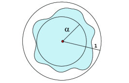
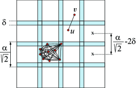
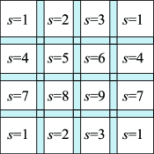
(a)	(b)	(c)

Figure 1: (a) The $\alpha$-QUDG model (b) Constructing a clique cover for $V$ (c) Clique ordering.

Let $0<\beta<\frac{\alpha}{\sqrt{2}}$ and $0<\delta<\beta/4$ be small constants to be fixed later. To compute a clique cover for $V$, we start by covering the plane with a grid of overlapping square cells of size $\beta\times\beta$, such that the distance between centers of adjacent cells is $\beta-2\delta$. Note that any two adjacent cells define a small band of width $\delta$ where they overlap. The reason for enforcing this overlap is to ensure that edges not entirely contained within a single grid cell are longer than $\delta$, i.e., they cannot be arbitrarily small. We identify each grid cell by the coordinates $(i,j)$ of its upper left corner. Any two vertices that lie within the same grid cell are no more than $\alpha$ distance apart and therefore are connected by an edge in $G$. This implies that the collection of vertices in each non-empty grid cell can be used to define a clique element of the clique cover. We call this particular clique cover a ($\beta,\delta$)-clique cover. Let $V_{1},V_{2},\ldots$ be the elements of the ($\beta,\delta)$-clique cover for $V$. Note that, since $\delta<\beta/4$, a node $u$ can belong to at most four subsets $V_{i}$.

Our LOS method consists of 4 steps. First we construct, for each $G[V_{i}]$, a $(1+\varepsilon)$-spanner of degree $O(1)$ and weight $O(\omega(MST(V_{i}))$. Various methods for constructing $H_{i}$ exist – for instance, the well-known sequential greedy method produces a spanner with the desired properties [8]. Second, we use the Yao method to generate $(1+\varepsilon)$-spanner paths between longer edges that span different grid cells. Third, we apply the reverse Yao step to reduce the number of Yao edges incident to each node. Finally, we apply a filtering method to eliminate all but a constant number of edges incident to a grid cell. This fourth step is necessary to ensure that the output spanner has bounded weight. These steps are described in detail in Table 3.

Algorithm LOS($G=(V,E),\varepsilon$)   {1. Compute a $(1+\varepsilon)$-spanner cover:} Fix $0<\beta<\frac{\alpha}{\sqrt{2}}$ and $0<\delta<\beta/4$. Compute a ($\beta,\delta$)-clique cover $V_{1},V_{2},\ldots$ for $V$. For each $i$, compute a $(1+\varepsilon)$-spanner $H_{i}$ for $G[V_{i}]$ using the method from [8]. Initialize $H=\cup_{i}H_{i}$. Let $E_{0}=\{uv\in E~{}|~{}uv\not\in G[V_{i}]$ for any $i$}. {2. Apply Yao on $E_{0}$:} Let $k$ be the smallest integer satisfying $\cos\frac{2\pi}{k}-\sin\frac{2\pi}{k}\geq\frac{\delta+1+\varepsilon}{(\delta+1)(1+\varepsilon)}$. For each node $u$, divide the plane into $k$ incident equal-size cones. Initialize $E_{Y}\leftarrow\emptyset$. For each cone $C_{u}$ such that $E_{0}\cap C_{u}$ is non-empty Pick the edge $uv\in E_{0}\cap C_{u}$ of smallest ID and add $\overrightarrow{uv}$ to $E_{Y}$. {3. Apply reverse Yao on $E_{Y}$:} Initialize $E_{YY}\leftarrow E_{Y}$. For each cone $C_{u}$ such that $E_{Y}\cap C_{u}$ is non-empty Discard from $E_{Y}$ all edges $\overrightarrow{vu}\in E_{Y}\cap C_{u}$, but the one of smallest ID. {4. Select connecting edges from $E_{YY}$:} Pick $r$ such that $r\leq\frac{(\delta+1)(1+\varepsilon)(\cos\theta-\sin\theta)-(\delta+1+\varepsilon)}{4}$, where $\theta=2\pi/k$. Compute an $r$-cluster cover for $V$ in $H$. Let $E_{1}\subseteq E_{YY}$ contain all Yao edges connecting cluster centers. Add $E_{1}$ to $H$. Output $H=(V,E_{H})$.

Table 3: The LOS algorithm.

Note that the Yao and reverse Yao steps are restricted to edges in the set $E_{0}$ whose aspect ratio is bounded above by $1/\delta$. The next three theorems prove the main properties of the LOS algorithm.

Theorem 2.1

The output $H$ generated by LOS($G,\varepsilon$) is a $(1+\varepsilon)$-spanner for $G$.

Proof

Let $uv\in E$ be arbitrary. If $uv\in G[V_{i}]$ for some $i$, then $H_{i}\subseteq H$ contains a $(1+\varepsilon)$-spanner $uv$-path (since $H_{i}$ is a $(1+\varepsilon)$-spanner for $G[V_{i}]$). Otherwise, $uv\in E_{0}$. The proof that $H$ contains a $(1+\varepsilon)$-spanner $uv$-path is by induction on the ID of edges in $E_{0}$. Let $uv\in E_{0}$ be the edge with the smallest ID and assume without loss of generality that ${\tt ID}(uv)={\tt ID}(\overrightarrow{uv})$. Since ${\tt ID}(uv)$ is smallest, $\overrightarrow{uv}$ gets added to $E_{Y}$ in step 2, and it stays in $E_{YY}$ in step 3. If $uv\in H$ at the end of step 4, then ${\tt sp}_{H}(u,v)=uv$. Otherwise, let $ab$ be the edge selected in step 4 of the algorithm, such that $u\in L_{a}$ and $v\in L_{b}$ (see Fig. 2a). Since $L_{a}$ and $L_{b}$ are both $r$-clusters, we have that $|{\tt sp}_{H}(u,a)|\leq r$ and $|{\tt sp}_{H}(v,b)|\leq r$. It follows that $|ua|\leq r$ and $|vb|\leq r$. By the triangle inequality, $|ab|<|uv|+2r$ and therefore ${\tt sp}_{H}(u,v)\leq|ab|+2r<|uv|+4r\leq(1+\varepsilon)|uv|$, for any $r\leq\delta\varepsilon/4$ (satisfied by the $r$ values restricted by the algorithm). This concludes the base case.

To prove the inductive step, let $uv\in E_{0}$ be arbitrary, and assume that $H$ contains $(1+\varepsilon)$-spanner paths between the endpoints of any edge whose ID is lower than ID($uv$).

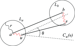
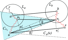
(a)	(b)

Figure 2: Thm. 2.1: (a) Base case. (b) ${\tt sp}_{H}(u,u_{1})\oplus{\tt sp}_{H}(u_{1},a)\oplus ab\oplus{\tt sp}_{H}(b,v_{1})\oplus{\tt sp}_{H}(v_{1},v)$ is a $(1+\varepsilon)$-spanner $uv$-path.

Let $uv_{1}\in C_{u}(v)$ be the Yao edge selected in step 2 of the algorithm; let $u_{1}v_{1}\in C_{v_{1}}(u)$ be the YaoYao edge selected in step 3 of the algorithm; and let $ab\in H$ be the edge added to $H$ in step 4 of the algorithm, such that $u_{1}\in L_{a}$ and $v_{1}\in L_{b}$ (see Fig. 2b). Note that $u$ and $u_{1}$ may be disjoint or may coincide, and similarly for $v$ and $v_{1}$. In either case, the chains of inequalities ${\tt ID}(u_{1}v_{1})\leq{\tt ID}(uv_{1})\leq{\tt ID}(uv)$ and $|u_{1}v_{1}|\leq|uv_{1}|\leq|uv|$ hold. Let $u^{\prime}_{1}$ be the projection of $u_{1}$ on $uv_{1}$. By the triangle inequality,

$$|uu_{1}|\leq|uu^{\prime}_{1}|+|u^{\prime}_{1}u_{1}|=|uv_{1}|-|u^{\prime}_{1}v_{1}|+|u^{\prime}_{1}u_{1}|\leq|uv_{1}|-|u_{1}v_{1}|\cos\theta+|u_{1}v_{1}|\sin\theta.$$ (1)

Similarly, if $v^{\prime}_{1}$ is the projection of $v_{1}$ on $uv$, we have

$$|v_{1}v|\leq|vv^{\prime}_{1}|+|v^{\prime}_{1}v_{1}|=|uv|-|uv^{\prime}_{1}|+|v^{\prime}_{1}v_{1}|\leq|uv|-|uv_{1}|\cos\theta+|uv_{1}|\sin\theta.$$ (2)

Since $|uu_{1}|<|uv_{1}|\leq|uv|$ and $|v_{1}v|<|uv|$, by the inductive hypothesis $H$ contains $(1+\varepsilon)$-spanner paths ${\tt sp}_{H}(u,u_{1})$ and ${\tt sp}_{H}(v_{1},v)$. Let $P_{1}={\tt sp}_{H}(u,u_{1})\oplus{\tt sp}_{H}(v_{1},v)$. The length of $P_{1}$ is

$$|P_{1}|\leq(1+\varepsilon)\cdot(|uu_{1}|+|v_{1}v|).$$

Substituting inequalities (1) and (2) yields

$$|P_{1}|\leq(1+\varepsilon)|uv|+(1+\varepsilon)|uv_{1}|(1-\cos\theta+\sin\theta)-(1+\varepsilon)|u_{1}v_{1}|(\cos\theta-\sin\theta).$$ (3)

Next we show that the path $P=P_{1}\oplus{\tt sp}_{H}(u_{1},a)\oplus ab\oplus{\tt sp}_{H}(b,v_{1})$ is a $(1+\varepsilon)$-spanner path from $u$ to $v$ in $H$, thus proving the inductive step. Using the fact that $|ab|<2r+|u_{1}v_{1}|$, $|{\tt sp}_{H}(u_{1},a)|\leq r$ and $|{\tt sp}_{H}(b,v_{1})|\leq r$, we get

$$|P|\leq|P_{1}|+|u_{1}v_{1}|+4r.$$ (4)

Substituting further $|u_{1}v_{1}|\geq\delta$ and $|uv_{1}|\leq 1$ in (3) and (4) yields

$$|P|\leq(1+\varepsilon)|uv|+(4r+(1+\varepsilon)(1-\cos\theta+\sin\theta)-\delta(1+\varepsilon)(\cos\theta-\sin\theta)-\delta).$$

Note that the second term on the right side of the inequality above is non-positive for any $r$ and $\theta$ satisfying the conditions of the algorithm:

$$\begin{cases}r\leq\frac{(\delta+1)(1+\varepsilon)(\cos\theta-\sin\theta)-(\delta+1+\varepsilon)}{4}\\ \cos\theta-\sin\theta>\frac{\delta+1+\varepsilon}{(\delta+1)(1+\varepsilon)}.\end{cases}$$

This completes the proof.  

Before proving the other two properties of $H$ (bounded degree and bounded weight), we introduce an intermediate lemma. For fixed $c>0$, call an edge set $F$ $c$-isolated if, for each node $u$ incident to an edge $e\in F$, the closed disk ${\tt disk}(u,c)$ centered at $u$ of radius $c$ contains no other endpoints of edges in $F$. This definition is a variant of the isolation property introduced in [10]. Das et al. show that, if an edge set $F$ satisfies the isolation property, then $\omega(F)$ is within a constant factor of the minimum spanning tree connecting the endpoints of $F$. Here we prove a similar result.

Lemma 1

Let $F$ be a $c$-isolated set of edges no longer than 1. Then $\omega(F)=O(1)\cdot\omega(T)$, where $T$ is the minimum spanning tree connecting the endpoints of edges in $F$.

Proof

Let $P$ be a Hamiltonian path obtained by a taking a preorder traversal of $T$. If each edge $uv\in P$ gets associated a weight value $\omega(uv)=|{\tt sp}_{T}(u,v)|$, then it is well-known that $\omega(P)\leq 2\omega(T)$. So in order to prove that $w(F)$ is within a constant factor of $\omega(T)$, it suffices to show that $\omega(F)=O(\omega(P))$. Since $F$ is $c$-isolated, the distance between any two vertices in $T$ is greater than $c$ and therefore $w(P)\geq(n-1)c$. On the other hand, no edge in $F$ is greater than 1 and therefore $\omega(F)\leq n$. It follows that $\omega(F)=O(\omega(P))$.  

Theorem 2.2

The output $H$ generated by running LOS($G,t$) has maximum degree $O(1)$ and total weight $O(1)\cdot\omega(MST)$.

Proof

The fact that $H$ has maximum degree $O(1)$ follows immediately from three observations: (a) each spanner $H_{i}$ constructed in step 1 of the algorithm has degree $O(1)$ [8], (b) a node $u$ belongs to at most four subgraphs $H_{i}$, and (c) a node $u$ is incident to a constant number of Yao edges (at most $2k$) [18].

We now prove that the total weight for $H$ is within a constant factor of $\omega(MST)$, which is optimal. The main idea is to partition the edge set $E_{H}$ into a constant number of subsets, each of which has low weight. Consider first the $(1+\varepsilon)$-spanners constructed in step 1 of the algorithm. Each $(1+\varepsilon)$-spanner $H_{\ell}$ corresponds to a grid cell $(i,j)$. Let $F$ denote the set of edges in $\cup_{\ell}H_{\ell}$. Define the edge set $F_{s}\subseteq F$ to contain all spanner edges corresponding to those grid cells $(i,j)$ whose indices $i$ and $j$ satisfy the condition $(i\mod 3)\times 3+j\mod 3=s$. Intuitively, if two edges $e_{1},e_{2}\in F_{s}$ lie in different grid cells, then those grid cells are separated by at least two other grid cells (see Fig. 1c). This further implies that the closest endpoints of $e_{1}$ and $e_{2}$ are distance $\alpha$ or more apart. Also notice that it takes only 9 subsets $F_{1},F_{2},\ldots,F_{9}$ to cover $F$.

Next we show that $\omega(F_{s})=O(\omega(T_{s}))$ for each $s=1,2,\ldots,9$, where $T_{s}$ is a minimum spanning tree connecting the endpoints in $F_{s}$. To see this, first observe that $F_{s}$ combines the edges of several low-weight $(1+\varepsilon)$-spanners $H_{s_{1}},H_{s_{2}},\ldots$ with the property that $\omega(H_{s_{1}})=O(\omega(T_{s_{1}}))$, where $T_{s_{1}}$ is a minimum spanning tree connecting the nodes in $H_{s_{1}}$. Thus, in order to prove that $\omega(F_{s})=O(\omega(T_{s}))$, it suffices to show $\sum_{i}\omega(T_{s_{i}})=O(\omega(T_{s}))$. We will in fact prove that

$$\sum_{i}\omega(T_{s_{i}})\leq\omega(T_{s})$$

We prove this by showing that, if Prim’s algorithm is employed in constructing $T_{s}$ and $T_{s_{i}}$, then $T_{s_{i}}\subseteq T_{s}$, for each $i$. Since the trees $T_{s_{i}}$ are all disjoint (separated by at least 2 grid cells), the claim follows. Recall that Prim’s algorithm processes edges by increasing length and adds them to $T_{s}$ as long as they do not close a cycle. This means that all edges shorter than $\alpha$ are processed before edges longer than $\alpha$. Let $e\in T_{s_{i}}$ be arbitrary. Then $|e|\leq\alpha$, since $T_{s_{i}}$ is restricted to one grid cell only of diameter $\alpha$. If $e\not\in T_{s}$, then it must be that $e$ closes a cycle $C$ at the time it gets processed. Note however that $C$ must lie entirely in the grid cell containing $T_{s_{i}}$, since $C$ contains edges no longer than $\alpha$, and all edges with endpoints in different cells are longer than $\alpha$. Furthermore, $C$ must contain an edge $e^{\prime}\not\in T_{s_{i}}$ such that $|e^{\prime}|\leq|e|$. The case $|e^{\prime}|=|e|$ cannot happen if Prim breaks ties in the same manner in both $T_{s}$ and $T_{s_{i}}$, so it must be that $|e^{\prime}|<|e|$. But then we could replace $e$ in $T_{s_{i}}$ by $e^{\prime}$, resulting in a smaller spanning tree, a contradiction. It follows that $e\in T_{s}$ and therefore $T_{s_{i}}\subseteq T_{s}$, for each $i$. This concludes the proof that $\omega(F_{s})=O(\omega(T_{s}))$, for each $s$. Since there are at most 9 such sets $F_{s}$ that cover $F$ and since $\omega(T_{s})\leq\omega(MST)$, we get that $\omega(F)=O(\omega(MST))$.

It remains to prove that $\omega(E_{H}\setminus F)=O(\omega(MST))$. Let $d\leq 2k$ be the maximum number of edges in $E_{H}\setminus F$ incident to any node in $H$. Partition the edge set $E_{H}\setminus F$ into no more than $2d\leq 4k$ subsets $E_{1},E_{2},\ldots$, such that no two edges in $E_{i}$ share a vertex, for each $i$. We now show that $\omega(E_{i})=O(\omega(MST))$, for each $i$. Since there are only a constant number of sets $E_{i}$ ($4k$ at most), it follows that $\omega(E_{H}\setminus F)=O(\omega(MST))$. The key observation to proving that $\omega(E_{i})=O(\omega(MST))$ is that any two edges $uv,ab\in E_{i}$ have their closest endpoints – say, $u$ and $a$ – separated by a distance of at least $r/t$. This is because $t|ua|\geq|{\tt sp}_{H}(u,a)|>r$; the first part of this inequality follows from the spanner property of $H$, and the second part follows from the fact that $u$ and $a$ are centers of different $r$-clusters (a property ensured by step 4 of the algorithm). This implies that $E_{i}$ is $r/t$-isolated, and by Lem. 1 we have that $\omega(E_{i})=O(\omega(MST))$.

We have established that $\omega(F)=O(\omega(MST))$ and $\omega(E_{H}\setminus F)=O(\omega(MST))$. It follows that $w(H)=w(E_{H})=O(\omega(MST))$ and this completes the proof.  

Theorem 2.3

The LOS algorithm can be implemented in $O(1)$ rounds of communication using messages that are $O(\log n)$ bits each.

Proof

Let $x_{u}$ and $y_{u}$ denote the coordinates of a node $u$. At the beginning of the algorithm, each node $u$ broadcasts the information $({\tt ID}(u),x_{u},y_{u})$ to its neighbors and collects similar information from its neighbors. Each node $u$ determines the grid cell(s) $(i,j)$ it belongs to from two conditions, $i\alpha/\sqrt{2}\leq x_{u}<(i+1)\alpha/\sqrt{2}$ and $j\alpha/\sqrt{2}\leq y_{u}<(j+1)\alpha/\sqrt{2}$. Similarly, for each neighbor $v$ of $u$, each node $u$ determines the grid cell(s) that $v$ belongs to. Thus step 1 of the algorithm can be implemented in one round of communication: using the information from its neighbors, each node $u$ computes the clique corresponding to those cells $(i,j)$ that $u$ belongs to (at most 4 of them), then $u$ computes a $(1+\varepsilon)$-spanner for each such clique by performing local computations. Note that knowledge of node coordinates is critical to implementing step 1 efficiently.

Step 2 (the Yao step) and step 3 (the reverse Yao step) of the algorithm are inherently local: each node $u$ computes its incident Yao and YaoYao edges based on the information gathered from its neighbors in step 1.

It remains to show that step 4 can also be implemented in $O(1)$ rounds of communication. We will in fact show that eight rounds of communication suffice to compute an $r$-cluster cover for $V$ in $H$. Define $U_{s}$ to be the set of vertices that lie in the grid cells $(i,j)$ such that $(i\mod 2)\times 2+j\mod 2=s$. This is the same as saying that two vertices that lie in different cells are about one grid cell apart. Note that $V=\cup_{s=1}^{4}U_{s}$. To compute an $r$-cluster cover for $V$, each node $u$ executes the ClusterCover method described below. For simplicity we assume that $r>\delta$, so that two cluster centers that lie in different grid cells are at least distance $r$ apart. However, the ClusterCover method can be easily extended to handle the situation $r\leq\delta$ as well.

Computing a ClusterCover($u,r$)   Repeat for $s=1,2,3,4$ (A) Collect information on cluster centers from neighbors (if any). If $u$ belongs to $U_{s}$ Let $V_{\ell}\subseteq U_{s}$ be the clique containing $u$ (computed in step 1 of LOS). (B) Broadcast information on existing cluster centers in $V_{\ell}$ to all nodes in $V_{\ell}$. (C) For each existing cluster center $w\in V_{\ell}$ Add to $C_{w}$ all uncovered nodes $v\in V_{\ell}$ such that ${\tt sp}_{H}(w,v)\leq r$. Mark all nodes in $C_{w}$ covered. (D) While $V_{\ell}$ contains uncovered nodes Pick the uncovered node $w\in V_{\ell}$ of highest ${\tt ID}$. Add to $C_{w}$ all uncovered nodes $v\in V_{\ell}$ such that ${\tt sp}_{H}(v,w)\leq r$. Mark all nodes in $C_{w}$ covered. (E) Broadcast the cluster centers computed in step (C) to all neighbors.

No information on existing cluster centers is available in the first iteration of the ClusterCover method (i.e, for $s=1$). Each node in $U_{1}$ skips directly to step (D), which implements the standard greedy method for computed an $r$-clique cover for a given node set ($V_{\ell}$ in our case). In the second iteration, some of the clusters computed during the first iteration might be able to grow to incorporate new vertices from $U_{2}$. This is particularly true for cluster centers that lie in the overlap area of two neighboring cells. Information on such cluster centers is distributed to all relevant nodes in step (E) in the first iteration, then collected in step (A) and forwarded to all nodes in $V_{\ell}$ in step (B) in the second iteration. This guarantees that all nodes in $V_{\ell}$ have a consistent view of existing cluster centers in $V_{\ell}$ at the beginning of step (C). Existing clusters grow in step (C), if possible, and new clusters get created in step (D), if necessary. This procedure shows that it takes no more than 8 rounds of communication to implement step 4 of the LOS algorithm. One final note is that information on a constant number of cluster centers is communicated among neighbors in steps (A), (B) and (D) of the ClusterCover method. This is because only a constant number of $r$-clusters can be packed into a grid cell. So each message is $O(\log n)$ bits long, necessarily so to include a constant number of node identifiers, each of which takes $O(\log n)$ bits.  

2.2 The PLOS Algorithm

In this section we impose our spanner to be planar, at the expense of a bigger stretch factor. This tradeoff is unavoidable, since there are UDGs that contain no $(1+\varepsilon)$-spanner planar subgraphs, for arbitrarily small $\varepsilon$ (a simple example would be a square of unit diameter).

Our PLOS algorithm consists of 4 steps. In a first step we construct the unit Delaunay triangulation ${\tt UDel}(V)$ using the method described in [21]. Remaining steps use the grid-based idea from Sec. 2.1 to refine the Delaunay structure. Let $V_{1},V_{2},\ldots$ be a $(\beta,\delta)$-clique cover for $V$, as defined in Sec. 2.1. In step 2 of the algorithm we apply the OrderedYao method on edge subsets of ${\tt UDel}$ incident to each clique $V_{i}$. The reason for restricting this method to each clique, as opposed to the entire spanner ${\tt UDel}(V)$ as in [32], is to reduce the total of $O(n)$ rounds of communication to $O(1)$. The individual degree of each node increases as a result of this alteration, however it remains bounded above by a constant. Steps 3 and 4 aim to reduce the total weight of the spanner. Step 3 uses a Greedy method to filer out edges with both endpoints in one same clique $V_{i}$. Step 4 uses clustering to filter out edges spanning multiple cliques. These steps are described in detail in Table 4.

Algorithm PLOS($G=(V,E),\varepsilon$)   {1. Start with the localized Delaunay structure for $G$:} Compute ${\tt LDel}=(V,E_{{\tt LDel}})$ for $G$ using the method from [21]. Fix $0<\beta\leq\frac{1}{\sqrt{2}}$ and $0<\delta<\frac{\beta}{4}$. Compute a ($\beta,\delta$)-clique cover $V_{1},V_{2},\ldots$ for $V$. {2. Bound the degree:} For each clique $V_{i}$ do the following: 2.1 Let $E_{i}\subseteq E_{{\tt UDel}}$ contain all unit Delaunay edges incident to nodes in $V_{i}$. 2.2 Execute ${\tt YDel}_{i}\leftarrow$ OrderedYao($G_{i}=(V,E_{i})$) (see Table 2). Set ${\tt YDel}=(V,E_{{\tt YDel}})=\bigcup_{i}{\tt YDel}_{i}$. {3. Bound the weight of edges confined to single grid cells:} Initialize $E_{H}=\emptyset$ and $H=(V,E_{H})$. Repeat for $k=1,2,3,4$ {Use Greedy on non-adjacent grid cells:} For each grid cell $L=L(i,j)$ such that $(i\mod 2)\times 2+j\mod 2=k$ 3.1 Let $E_{L}=E_{{\tt YDel}}\cap L$ contain all edges in YDel that lie in $L$. Let $E_{Q}=E_{{\tt YDel}}\setminus E_{L}$ and $Q=(V,E_{Q})$ define the query graph for $E_{L}$. 3.2 Sort $E_{L}$ in increasing order by edge ID. For each edge $e=uv\in E_{L}$, resolve a shortest path query: If ${\tt sp}_{Q}(u,v)>(1+\varepsilon)|uv|$ then add $uv$ to $H$ and $Q$. Otherwise, eliminate $uv$ from YDel. {4. Bound the weight of edges spanning multiple grid cells:} Pick $r$ such that $r\leq\frac{\varepsilon\delta}{4}$ and compute an $r$-cluster cover for ${\tt YDel}$. Add to $H$ those edges in YDel connecting cluster centers. Output $H=(V,E_{H})$.

Table 4: The PLOS algorithm.

The reason for breaking up step 3 of the algorithm into 4 different rounds (for $k=1,\ldots,4$) will become clear later, in our discussion of communication complexity (Thm. 2.8). We now turn to proving some important properties of the output spanner. We start with a preliminary lemma.

Lemma 2

The graph YDel constructed in step 2 of the PLOS algorithm is a planar $t_{1}$-spanner for $G$, for any $t_{1}>C_{del}(\frac{\pi}{2}+1)$. Furthermore, for each edge $ab\in G$, YDel contains a $t_{1}$-spanner $ab$-path with all edges shorter than $ab$ [32].

Proof

${\tt LDel}$ is a planar $C_{del}$-spanner for $G$ [21]. By Thm. 1.1, ${\tt YDel}_{i}$ is a planar $(\frac{\pi}{2}+1)$-spanner for $G_{i}$, for each $i$. These together with the fact that ${\tt LDel}=\bigcup_{i}G_{i}$ show that ${\tt YDel}$ is a $t_{1}$-spanner for $G$.

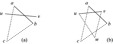
Figure 3: YDel is planar: edges $ab$ and $uv$ cannot cross.

The fact that ${\tt YDel}$ is planar follows an observation in [32] stating that, if a non-Delaunay edge $e\in{\tt YDel}$ crosses a Delaunay edge $e^{\prime}$, then $e^{\prime}$ must be longer than one unit and does not belong to YDel. More precisely, the following properties hold:

• A non-Delaunay edge $ab\in{\tt YDel}$ cannot cross a Delaunay edge $uv\in{\tt YDel}$. Recall that each non-Delaunay edge $ab\in{\tt YDel}$ closes an empty triangle $\triangle abc$ whose other two edges $ac$ and $bc$ are Delaunay edges. Thus, if $ab$ crosses $uv$, then at least one of $ac$ and $bc$ must cross $uv$, contradicting the planarity of LDel(see Fig 3a).

• No two non-Delaunay edges $ab,uv\in{\tt YDel}$ cross. The arguments here are similar to the ones above: if $ab$ and $uv$ intersect, then at least two of the incident Delaunay edges intersect, contradicting the planarity of LDel(see Fig. 3b).

The second part of the lemma follows from [32].  

Theorem 2.4

The output $H$ generated by PLOS($G,\varepsilon$) is a planar $t$-spanner for $G$, for any constant $t>C_{del}(1+\varepsilon)(1+\frac{\pi}{2})$.

Proof

Since $H\subseteq{\tt YDel}$, by Lem. 2 we have that $H$ is planar. We now show that $H$ is a $t$-spanner for $G$. The proof is by induction on the length of edges in $H$. The base case corresponds to the edge $uv\in G$ of smallest ID. Clearly $uv\in{\tt LDel}$, since $uv$ is a Gabriel edge. Also $uv\in{\tt YDel}$, since it has the smallest ID among all edges and therefore it belongs to the Yao structure for LDel. We now distinguish two cases:

• There is a grid cell containing both $u$ and $v$. In this case $uv\in H$, since $uv$ is the first edge queried by Greedy in step 3 and therefore it gets added to $H$.

• There is no grid cell containing both $u$ and $v$. Let $ab$ be the edge selected in step 4 of the algorithm, such that $u\in L_{a}$ and $v\in L_{b}$ (see Fig. 2a). Then arguments similar to the ones used for the base case of Thm. 2.1 show that ${\tt sp}_{H}(u,a)\oplus ab\oplus{\tt sp}_{H}(b,v)$ is a $(1+\varepsilon)$-spanner $uv$-path, for any $r\leq\varepsilon\delta/4$.

This concludes the base case. To prove the inductive step, pick an arbitrary edge $uv\in G$, and assume that $H$ contains $t$-spanner paths between the endpoints of each edge in $G$ of smaller ID. By Lem. 2, YDel contains a $\frac{t}{1+\varepsilon}$-spanner path $u=u_{0},u_{1},\ldots,u_{s}=v$:

$$\sum_{i=0}^{s}|u_{i}u_{i+1}|\leq\frac{t}{1+\varepsilon}|uv|$$ (5)

For each edge $u_{i}u_{i+1}\in{\tt YDel}$, one of the following cases applies:

• There is a grid cell containing both $u_{i}$ and $u_{i+1}$. In this case, the Greedy step (step 3 of the algorithm) guarantees that $|{\tt sp}_{H}(u_{i},u_{i+1})|\leq(1+\varepsilon)|u_{i}u_{i+1}|$.

• There is no grid cell containing both $u_{i}$ and $u_{i+1}$. Arguments similar to the ones for the base case show that $|{\tt sp}_{H}(u_{i},u_{i+1})|\leq(1+\varepsilon)|u_{i}u_{i+1}|$.

In either case, $H$ contains a $(1+\varepsilon)$-spanner $u_{i}u_{i+1}$-path. This together with (5) shows that

$$|{\tt sp}_{H}(u,v)|=\sum_{i=0}^{s}|{\tt sp}_{H}(u_{i},u_{i+1})|\leq(1+\varepsilon)\sum_{i=0}^{s}|u_{i}u_{i+1}|\leq t|uv|.$$

This completes the proof.  

Theorem 2.5

The output $H$ generated by PLOS has maximum degree $O(1)$.

Proof

Since $H\subseteq{\tt YDel}$, it suffices to show that the graph YDel constructed in step 2 of the PLOS algorithm has degree bounded above by a constant. By Thm. 1.1, the maximum degree of ${\tt YDel}_{i}$ is 25, for each $i$. Also note that unit disk centered at a node $u$ intersects $O(\frac{1}{\beta^{2}})$ grid cells, meaning that $u$ is a neighbor of nodes in $O(\frac{1}{\beta^{2}})$ grid cells and therefore belongs to a constant number of graphs ${\tt YDel}_{i}$. This implies that the maximum degree of $u$ is $25\cdot O(\frac{1}{\beta^{2}})$, which is a constant.  

Definition 1

[Leapfrog Property] For any $t\geq t^{\prime}>1$, a set $F$ of edges has the $(t^{\prime},t)$-leapfrog property if, for every subset $S=\{u_{1}v_{1},u_{2}v_{2},\ldots,u_{m}v_{m}\}$ of $F$,

$$t^{\prime}\cdot|u_{1}v_{1}|<\sum_{i=2}^{m}|u_{i}v_{i}|+t\cdot\Big{(}\sum_{i=1}^{m-1}|v_{i}u_{i+1}|+|v_{m}u_{1}|\Big{)}.$$ (6)

Das and Narasimhan [9] show the following connection between the leapfrog property and the weight of the spanner.

Lemma 3

Let $~{}t\geq t^{\prime}>1$. If the line segments $F$ in $d$-dimensional space satisfy the $(t^{\prime},t)$-leapfrog property, then $\omega(F)=O(\omega(MST))$, where $MST$ is a minimum spanning tree connecting the endpoints of line segments in $F$.

Lemma 4

At the end of each iteration $k$ in step 3 of the PLOS algorithm, for $k=1,\ldots,4$, $Q$ contains $(1+\varepsilon)^{k}$-spanner paths between the endpoints of any YDel edge processed in iterations 1 through $k$.

Proof

The proof is by induction on $k$. The base case corresponds to $k=1$. In this case, Greedy ensures that $Q$ contains a $(1+\varepsilon)$-spanner $uv$-path for each edge $uv$ processed in this iteration. This is because $uv\in{\tt YDel}$ either gets added to $Q$ in step 3.1 (and never removed thereafter), or gets queried in step 3.2. To prove the inductive step, consider a particular iteration $k>1$, and assume that the lemma holds for iterations $\ell=1\ldots k-1$. Again Greedy ensures that $Q$ contains a $(1+\varepsilon)$-spanner $uv$-path for each edge $uv$ processed in iteration $k$. Consider now an arbitrary edge $uv$ processed in iteration $\ell<k$. By the inductive hypothesis, at the end of round $k-1$, $Q$ contains a $(1+\varepsilon)^{k-1}$-spanner path $p(u,v)$. However, it is possible that $p(u,v)$ contains edges processed in round $k$ (since Greedy does not restrict $p(u,v)$ to lie entirely in the cell containing $uv$). For each such edge, Greedy ensures the existence of a $(1+\varepsilon)$-spanner path in $Q$. It follows that, at the end of iteration $k$, $Q$ contains a $(1+\varepsilon)^{k}$-spanner $uv$-path.  

Theorem 2.6

[Leapfrog Property] Let $L$ be an arbitrary grid cell and let $F\subseteq E_{L}$ be the set of edges with both endpoints in $L$ that get added to $H$ in step 3 of the algorithm. Then $F$ satisfies the $(1+\varepsilon,t)$-leapfrog property, for $t=(1+\varepsilon)^{4}(\frac{\pi}{2}+1)C_{del}$.

Proof

Consider an arbitrary subset $S=\{u_{1}v_{1},u_{2}v_{2},\ldots,u_{m}v_{m}\}\subseteq F$. To prove inequality (6) for $S$, it suffices to consider the case when $u_{1}v_{1}$ is a longest edge in $S$. Define $S^{\prime}=\{v_{m}u_{1}\}\cup\{v_{\ell}u_{\ell+1}~{}|~{}1\leq\ell<s\}$. Since $u_{i}$ and $v_{i}$ lie in $L$ for each $i$, all edges from $S^{\prime}$ lie entirely in $L$. Let $ab\in S^{\prime}$ be arbitrary. If $|ab|\geq|u_{1}v_{1}|$, then inequality (6) trivially holds, so assume that $|ab|<|u_{1}v_{1}|$. Next we show that $Q$ contains an $ab$-path of length no greater than $t|ab|$ at the time $\{u_{1},v_{1}\}$ gets queried. We distinguish two cases:

• $ab\in{\tt YDel}$. In this case $ab$ gets queried in step 3 prior to $u_{1}v_{1}$, meaning that $Q$ contains a path $P_{Q}(a,b)$ of length $|P_{Q}(a,b)|\leq(1+\varepsilon)^{4}|ab|$, at the time $u_{1}v_{1}$ gets queried (by Lem. 4).

• $ab\not\in{\tt YDel}$. By Lem. 2, ${\tt YDel}$ contains a path $P_{{\tt YDel}}(a,b)$ of length

  $$|P_{{\tt YDel}}(a,b)|\leq\frac{t}{(1+\varepsilon)^{4}}|ab|$$ (7)

  that contains only edges shorter than $ab$. For each edge $pq\in P_{{\tt YDel}}(a,b)$, $Q$ contains a path $P_{Q}(p,q)$ of length $|P_{Q}(p,q)\leq(1+\varepsilon)^{4}|pq|$, at the time $u_{1}v_{1}$ gets queried (by Lem. 4). Thus we have that

  $$|P_{Q}(a,b)|=\sum_{pq\in P_{{\tt YDel}}(a,b)}|P_{Q}(p,q)|\leq(1+\varepsilon)^{4}\sum_{pq\in P_{{\tt YDel}}(a,b)}|pq|\leq t|ab|$$ (8)

  This latter inequality follows from (7).

For $1\leq k<s$, let $P_{\ell}$ be a shortest $v_{\ell}u_{\ell+1}$-path in $Q$, and let $P_{m}$ be a shortest $v_{m}u_{1}$-path in $Q$. By the arguments above, such paths exists in $Q$ at the time $u_{1}v_{1}$ gets queried, and their stretch factor does not exceed $t$. Then $P=P_{1}\oplus u_{2}v_{2}\oplus P_{2}\oplus u_{3}v_{3}\oplus\ldots\oplus P_{m}$ is a path from $u_{1}$ to $v_{1}$ in $Q$, and $\omega(P)$ is no greater than the right hand side of the leapfrog inequality (6). Furthermore, $\omega(P)>(1+\varepsilon)|u_{1}v_{1}|$, otherwise the edge $u_{1}v_{1}$ would not have been added to $H$ (and $Q$) in step 3 of the algorithm. This concludes the proof.  

Theorem 2.7

The output $H$ generated by PLOS has total weight $O(\omega(MST))$.

Proof

The proof is very similar to the proof of Thm. 2.2 and uses the results of Lem. 3 and Thm.2.6.  

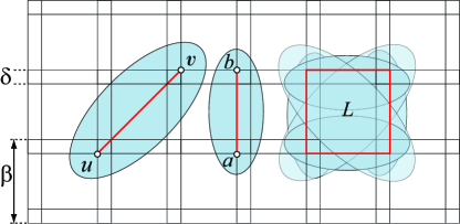
Figure 4: Valid ranges for $|{\tt sp}_{H}(u,v)|\leq(1+\varepsilon)|uv|$ queries (step 3 of the PLOS algorithm), illustrated for $\varepsilon=1/2$: query range for edge $uv$ (left), for edge $ab$ (middle), and for the entire grid cell $L$ (right).

Lemma 5

For any $\varepsilon<2$, the shortest path query $|{\tt sp}_{Q}(u,v)|\leq(1+\varepsilon)|uv|$ in step 3 of the PLOS algorithm involves only those grid cells incident to the cell $L$ containing $uv$.

Proof

For a fixed edge $uv$, the locus of all points $z$ with the property that $|uz|+|zv|\leq(1+\varepsilon)|uv|$ is a closed ellipse $A$ with focal points $u$ and $v$. Clearly, a point exterior to $A$ cannot belong to a $(1+\varepsilon)$-spanner path $p(u,v)$ from $u$ to $v$, so it suffices to limit the search for $p(u,v)$ to the interior of $A$. Fig. 4 (left and middle) shows the search domains for edges corresponding to one diagonal ($uv$) and one side ($ab$) of a grid cell. For any grid cell $L$, the union of $L$ and the search ranges for the two diagonals and four sides of $L$ covers the search domain for any edge that lies entirely in $L$ (see Fig. 4 right). It can be easily verified that, for $\varepsilon<2$, the search domain for $L$ fits in the union of $L$ and its eight surrounding grid cells.  

Theorem 2.8

The PLOS algorithm can be implemented in $O(1)$ rounds of communication.

Proof

Computing LDel in step 1 of the algorithm takes at most 4 communication rounds [21]. As shown in the proof of Thm. 2.2, computing the clique cover in step 1 takes at most 8 rounds of communication. Step 2 of the algorithm is restricted to cliques. A node $u$ belongs to at most 4 cliques. For each such clique, $u$ executes step 2 locally, on the neighborhood collected in step 1. In a few rounds of communication, each node $u$ is also able to collect the information on the grid cells incident to the ones containing $u$. By Lem. 5, this information suffices to execute step 4 of the algorithm locally.  

3 Conclusions

We present the first localized algorithm that produces, for any given QUDG $G$ and any $\varepsilon>0$, a $(1+\varepsilon)$-spanner for $G$ of maximum degree $O(1)$ and total weight $O(\omega(MST))$, in $O(1)$ rounds of communication. We also present the first localized algorithm that produces, for any given UDG $G$, a planar $O(1)$-spanner for $G$ of maximum degree $O(1)$ and total weight $O(\omega(MST))$, in $O(1)$ rounds of communication. Both algorithms require the use of a Global Positioning System (GPS), since each node uses its own coordinates and the coordinates of its neighbors to take local decisions. Our work leaves open the question of eliminating the GPS requirement without compromising the quality of the resulting spanners.

References

- [1] F. Araújo and L. Rodrigues. Fast localized Delaunay triangulation. In OPODIS, pages 81–93, 2004.
- [2] P. Bose, L. Devroye, W. Evans, and D. Kirkpatrick. On the spanning ratio of Gabriel graphs and beta-skeletons. SIAM J. of Discrete Mathematics, 20(2):412–427, 2006.
- [3] P. Bose, J. Gudmundsson, and M. Smid. Constructing plane spanners of bounded degree and low weight. In ESA ’02: Proc. of the 10th Annual European Symposium on Algorithms, pages 234–246, London, UK, 2002. Springer-Verlag.
- [4] P. Bose, P. Morin, I. Stojmenovic, and J. Urrutia. Routing with guaranteed delivery in ad hoc wireless networks. Wireless Networks, 7(6):609–616, 2001.
- [5] M. Burkhart, P. von Rickenbach, R. Wattenhofer, and A. Zollinger. Does topology control reduce interference? In MobiHoc ’04: 5th ACM Int. Symposium of Mobile Ad Hoc Networking and Computing, pages 9–19, 2004.
- [6] M. Damian. A simple Yao-Yao-based spanner of bounded degree. http://arxiv.org/abs/0802.4325v2, 2008.
- [7] G. Das and D. Joseph. Which triangulations approximate the complete graph? In Proceedings of the international symposium on Optimal algorithms, pages 168–192, New York, NY, USA, 1989. Springer-Verlag New York, Inc.
- [8] G. Das and G. Narasimhan. A fast algorithm for constructing sparse Euclidean spanners. Int. J. Comput. Geometry Appl., 7(4):297–315, 1997.
- [9] G. Das and G. Narasimhan. A fast algorithm for constructing sparse Euclidean spanners. Int. Journal on Computational Geometry and Applications, 7(4):297–315, 1997.
- [10] G. Das, G. Narasimhan, and J. Salowe. A new way to weigh malnourished Euclidean graphs. In SODA ’95: Proceedings of the sixth annual ACM-SIAM symposium on Discrete algorithms, pages 215–222, Philadelphia, PA, USA, 1995. Society for Industrial and Applied Mathematics.
- [11] D. P. Dobkin, S. J. Friedman, and K. J. Supowit. Delaunay graphs are almost as good as complete graphs. Discrete and Computational Geometry, 5(4):399–407, 1990.
- [12] K.R. Gabriel and R.R. Sokal. A new statistical approach to geographic variation analysis. Systematic Zoology, 18:259–278, 1969.
- [13] J. Gao, L. Guibas, J. Hershberger, L. Zhang, and A. Zhu. Geometric spanner for routing in mobile networks. In MobiHoc ’01: Proc. of the 2nd ACM Int. Symposium on Mobile Ad Hoc Networking and Computing, pages 45–55, 2001.
- [14] J. Gudmundsson and C. Knauer. Dilation and detours in geometric networks. In T.F. Gonzalez, editor, Handbook on Approximation Algorithms and Metaheuristics, Boca Raton, 2006. Chapman & Hall/CRC.
- [15] T. Johansson and L. Carr-Motyčková. Reducing interference in ad hoc networks through topology control. In DIALM-POMC ’05: Proc. of the joint workshop on Foundations of mobile computing, pages 17–23, 2005.
- [16] B. Karp and H. T. Kung. Greedy perimeter stateless routing for wireless networks. In MobiCom ’00: Proc. of the 6th Annual ACM/IEEE Int. Conference on Mobile Computing and Networking, pages 243–254, 2000.
- [17] J.M. Keil and C.A. Gutwin. The Delaunay triangulation closely approximates the complete Euclidean graph. Discrete and Computational Geometry, 7:13–28, 1992.
- [18] X. Li, P. Wan, Y. Wang, and O. Frieder. Sparse power efficient topology for wireless networks. In HICSS’02: Proc. of the 35th Annual Hawaii Int. Conference on System Sciences, volume 9, page 296.2, 2002.
- [19] X.-Y. Li. Approximate MST for UDG locally. In COCOON’03: Proc. of the 9th Annual Int. Conf. on Computing and Combinatorics, pages 364–373, 2003.
- [20] X. Y. Li, G. Calinescu, and P. Wan. Distributed construction of planar spanner and routing for ad hoc wireless networks. In InfoCom ’02: Proc. of the 21st Annual Joint Conference of the IEEE Computer and Communications Societies, volume 3, 2002.
- [21] X. Y. Li, G. Calinescu, P. J. Wan, and Y. Wang. Localized Delaunay triangulation with application in ad hoc wireless networks. IEEE Trans. on Parallel and Distributed Systems, 14(10):1035–1047, 2003.
- [22] X.-Y. Li, Y. Wang, and W.-Z. Song. Applications of k-local mst for topology control and broadcasting in wireless ad hoc networks. IEEE Trans. on Parallel and Distributed Systems, 15(12):1057–1069, 2004.
- [23] X.Y. Li and Y. Wang. Efficient construction of low weight bounded degree planar spanner. In COCOON ’04: Proc. of the 9th Int. Computing and Combinatorics Conference, 2004.
- [24] J.C. Hou N. Li and L. Sha. Design and analysis of a MST-based topology control algorithm. In IEEE INFOCOM, 2003.
- [25] G. Narasimhan and M. Smid. Geometric Spanner Networks. Cambridge University Press, New York, NY, USA, 2007.
- [26] R. Rajaraman. Topology control and routing in ad hoc networks: a survey. SIGACT News, 33(2):60–73, 2002.
- [27] M. Smid. Closest-point problems in computational geometry. In J.-R. Sack and J. Urrutia, editors, Handbook of Computational Geometry, pages 877–935, Amsterdam, 2000. Elsevier Science.
- [28] W. Z. Song, Y. Wang, X. Y. Li, and O. Frieder. Localized algorithms for energy efficient topology in wireless ad hoc networks. In MobiHoc ’04: Proc. of the 5th ACM Int. Symposium on Mobile Ad Hoc Networking and Computing, pages 98–108, 2004.
- [29] G.T. Toussaint. The relative neighborhood graph of a finite planar set. Pattern Recognition, 12(4):261–268, 1980.
- [30] P. von Rickenbach, S. Schmid, R. Wattenhofer, and A. Zollinger. A robust interference model for wireless ad-hoc networks. In IPDPS ’05: Proc. of the 19th IEEE Int. Parallel and Distributed Processing Symposium - workshop 12, page 239.1, 2005.
- [31] P.-J. Wan, G. Calinescu, X.-Y. Li, and O. Frieder. Minimum energy broadcast routing in static ad hoc wireless networks. ACM Wireless Networking (WINET), 8(6):607–617, November 2002.
- [32] Y. Wang and X. Y. Li. Localized construction of bounded degree and planar spanner for wireless ad hoc networks. In Proc. of the Joint Workshop on Foundations of Mobile Computing, pages 59–68, 2003.
- [33] A.C.-C. Yao. On constructing minimum spanning trees in -dimensional spaces and related problems. SIAM Journal on Computing, 11(4):721–736, 1982.
- [34] M. Zuniga and B. Krishnamachari. An analysis of unreliability and asymmetry in low-power wireless links. ACM Trans. of Sensor Networks, 3(2), 2007.