Time Variation of Rotation Measure Gradient in 3C 273 Jet

Abstract

The existence of a gradient in the Faraday rotation measure (RM) of the quasar 3C 273 jet is confirmed by follow-up observations. A gradient transverse to the jet axis is seen for more than 20 mas in projected distance. Taking account of the viewing angle, we estimate it to be more than 100 pc. Comparing to the distribution of the RM in 1995, we detect a time variation of it at the same distance from the core over 7 yr. We discuss the origin of the Faraday rotation based on this rapid time variation. We rule out foreground media such as a narrow-line region, and suggest a helical magnetic field in the sheath region as the origin of this gradient of the RM.

1 Introduction

A gradient of the Faraday rotation measure (RM) across a jet is growing evidence for the existence of a toroidal or helical magnetic field associated with the jet. The first evidence for such a gradient of the RM across a jet was found by VLBA polarimetry toward the VLBI jet of a well-known quasar, 3C 273 (Asada et al. 2002, hereafter A02). Following this report, the same kind of gradient of the RM was reported for several jets of BL Lac objects (Gabuzda et al. 2004), and the gradient of the RM across the 3C 273 jet itself was also confirmed by several observations (Zavala & Taylor 2005; Attridge et al. 2005). The role of a toroidal or helical magnetic field has been discussed for the launching and propagating mechanisms of jets based on magnetohydrodynamics from the theoretical point of view (e.g., Meier et al. 2001 and references therein), and it has been suggested that the presence of a toroidal or helical magnetic field could be observed as a gradient of the RM across the jet (Blandford 1993). Recently, it has also been shown that the toroidal magnetic field in a jet’s rest frame would be observed as a toroidal magnetic field in the observer frame with a compression of the pitch angle (Lyutikov et al. 2005). In this paper we report on our follow-up observation, which confirms our initial results and indicates a time variation. Throughout this paper, we use a Hubble constant of H₀ = 100 km s^-1 Mpc^-1 and a deceleration parameter of q₀ = 0.5 in order to keep consistency to the previous papers (e.g., A02). An angular resolution of one milli-arcsecond (mas) corresponds to a linear resolution of 1.86 pc.

2 Observations and Data Reductions

Observations were carried out on 2002 December 15 using all 10 stations of the VLBA. Spacing the sampling by multiples of the fundamental separation in $\lambda^{2}$ space was useful in order to avoid the 2$\pi$ ambiguity when we measured the RM at discrete observing wavelengths. In order to arrange the observing wavelengths in $\lambda^{2}$ space within an observing band, we chose intermediate frequencies ( IFs) of 4.618, 4.688, 4.800, and 5.093 GHz in the 5 GHz band, and 8.118, 8.188, 8.402, and 8.593 GHz in the 8 GHz band. Each IF had an 8 MHz bandwidth. Both left and right circular polarizations were recorded at each station. The integration time toward 3C 273 was 66 minutes at each frequency band. We observed OQ 208 as an instrumental calibration source, and 3C 279 and 4C 29.45 as polarization position angle calibration sources.

An a priori amplitude calibration for each station was derived from a measurement of the antenna gain and system temperatures during each run. Fringe fitting was performed on each IF and polarization independently using the AIPS task fring. After deriving the delay and rate difference between parallel-hand cross-correlations (between LHCP-LHCP or RHCP-RHCP), the cross-hand correlations (between LHCP-RHCP) were fringe-fitted to determine the cross-hand delay difference. Once the cross-hand delay difference was determined, full self-calibration was performed for the parallel-hand cross-correlations. Images were initially obtained using DIFMAP, and then imported into AIPS to self-calibrate the full data sets using the task calib to get a final DIFMAP image. The instrumental polarizations of the antennas were determined for each IF at each band with OQ 208, using the AIPS task lpcal. The polarization angle offset at each station was calibrated using observations of 3C 279 obtained in the VLA/VLBA Polarization Calibraton Monitoring Program (Myers & Taylor). The source was observed on 2002 December 17 by the VLA at 4.8851 and 4.8451 GHz, and 8.4351 and 8.4851 GHz. Any change in the source between the two observations is presumably small, since the observations were made with the VLA and VLBA with in 2 days of each other. The observing frequencies were slightly different between the VLA and VLBA observations, and the VLBA polarization position angles were interpolated using the VLA polarization position angle. In order to obtain the distributions of RM and projected magnetic field, we restored images at higher frequencies to match the resolution at the lowest frequency observation. The restored beam size was 3.22 mas $\times$ 1.23 mas with the major axis at a position angle of - 4.^∘63.

For the registration of images at different frequencies, we identified four distinct components. We measured the relative position with respect to the core component, peak flux, integrated flux, and size with the AIPS task imfit. As the core position may shift with frequency because of synchrotron self-absorption (Blandford & Königl 1979), we used optically thin components to register the images at different frequencies. We derived the positions of these components by weighted signal-to-noise ratios. The variances of the positions of the optically thin components are 0.059 mas in right ascension and 0.061 mas in declination. Those are 0.05 and 0.02 times the beam size, respectively. The distribution of the RM was obtained by the AIPS task RM with polarization images at 4.618, 5.093, 8.118, and 8.593 GHz, with regions where the polarized intensity is greater than 3 times the rms noise in the polarized intensity.

3 Results

3.1 Apparent Motions

The distribution of the RM is shown superposed on the distribution of the total intensity at the first (A02) and second epochs in Figure 1. Five components in the jet are identified, and are labeled in the same manner as at the first epoch. Apparent velocities $\beta_{app}$ are measured with respect to the core component D and the detailed parameters are listed in table 1. The components C1, C2, and C3 correspond to the components F, D, and B in independent measurements from the NRAO 2 cm survey (Kellermann et al. 2004), respectively. The measured apparent velocities are in good agreement with each other. The velocities measured by Kellermann et al. (2004) are used in the following discussion, since the velocities measured by ourselves are based on just two epoch measurements at lower frequency.

The viewing angle of the jet can be constrained from the Doppler effect by equation $\theta_{max}=2\arctan{1/\beta_{app}}$, where $\theta_{max}$ is the upper limit of the viewing angle between the jet and line of sight. The $\theta_{max}$ for components C1, C2 and C3 is 23.5^∘ $\pm$ 2.1^∘, 22.6^∘ $\pm$ 2.6^∘, and 17.8^∘ $\pm$ 0.3^∘, respectively.

3.2 RM distribution

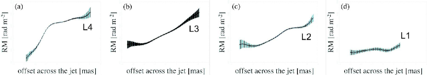
Figure 2: Cross sections of the RM distribution across (a) C3, (b) upper side of C2, (c) lower side of C2, and (d) C1 in the second epoch derived using the AIPS task SLICE (see line L1, L2, L3 and L4 in figure 1). The shaded area along the curved line of RM indicates the standard deviation (1 $\sigma$) in RM. The profile of the RM distribution is anti-symmetric with respect to the central axis of the jet.

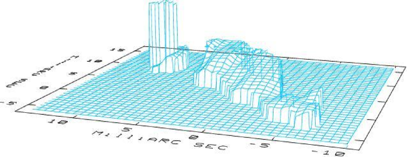
Figure 3: Bird’s eye view of the distribution of RM. Gradient of RM can be clearly seen in both transverse and along the jet axis.

The longer integration time toward 3C 273 brings us a better $u-v$ coverage at this epoch compared to the first epoch; thus we can reveal the distribution of the RM on a large part of the jet. We show the cross section of the RM at the second epoch along several lines perpendicular to the jet in Figure 2, and the RM distribution in a bird’s-eye view in Figure 3. We detected gradients in the RM up to 20 mas from the core at the second epoch, which corresponds to 38.4 pc in projected distance. Taking into account the upper limit of the viewing angle of the jet of component C2 of 22.6, the linear distance is longer than 100 pc.

The value of the RM is typically a few hundred rad m^-2, always positive, and the RM on the left side is larger by a few hundred rad m^-2 than on the right side. The trend of the gradient of the RM is consistent with our previous results (A02) and independent results by Zavala & Taylor (2005) and Attridge et al. (2005). However, the typical value of the RM observed by Zavala & Taylor is in the range from 0 to 2000 rad m^-2 in the region where we detect the RM gradient. This RM value is obviously larger than given by our observations. Two possibilities are suggested. One is that there is an averaging effect for low-frequency observations (Zavala & Taylor 2005). The other is that there is a real time variation of the distribution of the RM (Attridge et al. 2005). The possibility of a time variation of the RM is discussed in the following section.

On the other hand, even in our RM map only, a decreases in the RM from the core to the jet is seen (see Fig 3). This tendency is also consistent with RM of 22000 rad m^-2 at innermost components of 1 mas from the Stokes $I$ peak of the map by Attridge et al. (2005).

4 Discussions

Since the amount of Faraday rotation is larger than 90^∘ and the fractional polarization is reasonably strong, the magnetized plasma which is responsible for this Faraday rotation should be located in front of the emitting region. What makes this RM gradient? Two possibilities can be addressed. One is that the plasma is closely associated with the visible jet, as suggested by A02. The other is that foreground plasma independent of the jet produces the RM gradient by chance, as suggested by Gómez et al. (2000). Time variation of the RM distribution could address this issue.

First we consider the case in which the RM is produced by a magnetized plasma in a foreground screen that has nothing to do with the jet itself. Even a magnetized plasma in a narrow-line region (NLR) may not show variations in the Faraday screen on these short timescales, for the following reasons. It is well known that magnetized plasma in a NLR typically has a velocity of 1000 km $s^{-1}$. At the distance of 3C 273, this motion corresponds to 0.00056 mas yr^-1. The estimated motion between the two epochs (7 yr apart) would be 0.004 mas. This is too small to detect, and would not cause time variation in a foreground screen. Also, a change of the density in the magnetized plasma and/or magnetic field could not produce a time variation. Therefore, the characteristic timescale of the change in the RM should be related to the size of the magnetized plasma and the sound velocity or Alfvén velocity. Assuming a plasma temperature in the NLR of 10⁴ K and an equipartition condition for the magnetic pressure and thermal pressure, we estimate the Alfvén velocity and the sound speed to be 4 $\times$ 10^-5 c and 7 $\times$ 10^-5 c, respectively. If we assume a scale length for the magnetized plasma of 1 pc, the typical timescale of the variation in the foreground screen is estimated to be 8 $\times$ 10⁴ yr and 4 $\times$ 10⁴ yr, respectively.

Second we consider the RM being caused by magnetized plasma associated with the jet itself. In this case we expect the sheath around the emitting jet to be the origin of the RM (Inoue et al. 2003), since we do not see internal Faraday rotation. The sheath would be slower than the spine, but would have a relativistic velocity, since we do not detect any emission from the sheath at the counterjet. In addition, a highly time variable RM distribution would be expected due to the interaction between the spine and the sheath (Wardle et al. 2006).

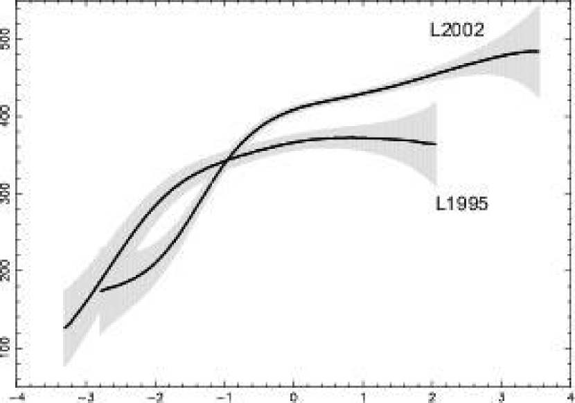
Figure 4: The cross sections of RM across the position at 9 mas from the core at both epochs are show (see line L1995 and L2002 in figure 1.). L1995 indicates the cross section at the first epoch and L2002 indicates that at the second epoch. The shade area shows three times the standard deviation (3 $\sigma$) in RM. There are the same trend of the gradient across the jet. However, RM at the second epoch is obviously larger than that at the first epoch.

We show the cross section of the RM at a distance of 9 mas from the core at both epochs in Figure 4 (see also Fig. 1). The slice of RM in 2002 is clearly different from that in 1995, and we think we detect time variation of the RM toward the jet between these epochs. In addition, we evaluate the registration error effect on the time variation of the RM as follows. First we assume that there are no time variations of the RM distribution between the two epochs, but there may be apparent time variations due to the registration error. In this case we would find a position where the RM distributions show a good pattern matching within the registration error. For this purpose, we tentatively shift the distribution of the RM of the first epoch up to $\pm$ 1 mas in right ascension and declination with respect to that of the second epoch, and calculate the reduced $\chi^{2}$ for each shifted position. We note that 1 mas is large compared to the registration error of one-fifth of the synthesized beam width. This calculation was performed only for shifts of the pixels where both distributions of the RM had a significant value (SNR $>$ 3) and the integrated area was larger than 3 times the synthesized beam size of the first epoch. The reduced $\chi^{2}$ larger than 4.0 was obtained all over the jet, suggesting that the two RM distributions are not identical, or that they changed with the jet evolution.

Zavala & Taylor (2001, 2005) reported that they did not detect time variation in the front of the jet, while they detected it toward the core over 6 months. The difference between our result and theirs would simply be due to the difference of the span between the two epochs and the choice of the observation frequencies. Since we observed at lower frequencies with the VLBA, it made it easy to detect small differences in the RM. In order to detect small differences in the RM, observations at lower frequencies with high angular resolution are necessary. Even if the RM is produced by a magnetized plasma in a foreground screen, the RM may also change if a relativistically moving polarized jet component is seen through a patchy foreground Faraday screen (Zavala & Taylor 2001). If this is the case, a repeatable distribution of the RM should be expected when the moving polarized jet component is located at the same position, as reported toward 3C 120 (Gómez et al. 2000; J. L. Gómez et al. 2006, private communication). We cannot check for any repeatability of the Faraday screen effect, since our analysis is based on only two-epoch observations. Therefore, it is not possible to discriminate between these two possibilities; a helical magnetic field associated with the jet or enhancement of the density in a foreground plasma. If the deconvolved size of the emitting knot and the typical scale of the foreground screen were smaller than the beam size, a rapid time variation of the RM would be expected. As the deconvolved size of the emitting knot is larger than the beam size, we expect the emission from the moving polarized jet to be traveling through the same foreground plasma at both epochs. We think that the time variation of the RM gradient is not associated with an enhancement of the density in a foreground plasma; therefore, a helical magnetic field in the sheath is preferable as the origin of the RM gradient. As is discussed with the first-epoch result (A02), the RM gradient can be explained using a helical magnetic field. Since the RM at the southeast side of the jet is larger than that at the northwest side, the direction of the toroidal component is clockwise seen from the core toward the downstream of the jet. In addition, if we assume that the offset of the RM is ascribed to the longitudinal component of the helical magnetic field, the helicity of the field can be estimated to be right-handed. Thus, we could define the helicity of the helical magnetic field and the direction of the rotation of the accretion disk or spinning black hole itself as clockwise as we see it. Therefore, we propose that a helical magnetic field in the sheath is responsible for the time-variable RM, and our monitoring program will answer this question, describing the characteristics of the time variation of the RM distribution in the 3C 273 jet.

5 Conclusions

In order to confirm the RM gradient across the 3C 273 jet, we made a follow-up observation using multifrequency VLBA polarimetry. The systematic gradient across the jet is confirmed for more than 100 pc along the jet, and the trend of the RM gradient is consistent with that revealed by previous observations. Since the amounts of the Faraday rotation exceed 90^∘, the origin of the Faraday rotation should be in the foreground of the emitting jet. On the other hand, we detected a time variation in the distribution of the RM in comparison to that in 1995, and this rapid time variation rules out the possibility that a foreground magnetized cloud independent of the jet, such as a narrow-line region, is responsible for the origin of the Faraday rotation. Therefore, the sheath around the ultra-relativistic jet is likely to be the origin.

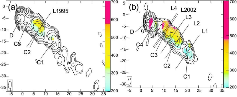
Figure 1: (a) Distribution of RM (color scale) superposed on the contour images of the total intensity at 4.760 GHz at the first epoch. Contours are plotted at -1, 1, 2, 4, 8, 16, 32, 64, 128, 256, 512 and 1024 $\times$ three-times the r.m.s. noise of that of the total intensity at 4.760 GHz. The synthesized beam size is 3.4 mas $\times$ 1.4 mas with the major axis at a position angle of - 3^∘.7. (b) Distribution of RM (color scale) superposed on the contour images of the total intensity at 4.618 GHz at the second epoch. Contours are plotted at -1, 1, 2, 4, 8, 16, 32, 64, 128, 256, 512 and 1024 $\times$ three-times the r.m.s. noise of that of the total intensity at 4.618 GHz. The synthesized beam size is 3.2 mas $\times$ 1.2 mas with the major axis at a position angle of - 4^∘.7. The RMs are plotted in the region where the polarized intensity is greater than 3-times the r.m.s. noise in the polarized intensity. Line L1995 in figure 1 (a) and L1, L2, L3, L4, and L2002 in figure 1 (b) show the position of the cross-sections shown in figure 2 and figure 4.

Table 1: Apparent proper motion

Component	$\beta_{app}$	$\beta_{app}$ by KK04	$\theta_{max}$
C1	5.9 $\pm$ 0.6	4.8 $\pm$ 0.9	23∘.5 $\pm$ 2∘.1
C2	5.3 $\pm$ 0.6	5.0 $\pm$ 1.2	22∘.6 $\pm$ 2∘.6
C3	7.2 $\pm$ 0.6	6.4 $\pm$ 0.2	17∘.8 $\pm$ 0∘.3

References

- (1) Asada, K., et al. 2002, PASJ, 54, 39L
- (2) Attridge, J. M., Wardle, J. F. C., & Homan, D. C. 2005, ApJL 633, 85
- (3) Blandford, R. D. 1993, in Astrophysical Jets, ed. D. Burgarella, M. Livio, & C. P. O’Dea (Cambridge: Cambridge Univ. Press), 1
- (4) Blandford, R. D. & Konigl, A. 1979, ApJ, 232, 34
- (5) Gabuzda, D. C., Murray, E. & Cronin, P. 2004, MNRAS, 351, L89
- (6) Gómez, J.L. et al. 2000, Science, 289, 2317
- (7) Inoue, M. et al. 2003, Radio Astronomy at the Fringe, ASP Conference Proceedings, Vol. 300, 141
- (8) Kellermann, K. I., Lister, M. L., Homan, D. C., Vermeulen, R. C., Cohen, M. H., Ros, E., Kadler, M., Zensus, J. A., & Kovalev, Y. Y. 2004, ApJ, 609, 539
- (9) Lyutikov, M., Pariev, V. I., & Gabuzda, D. C. 2005, MNRAS, 360, 869
- (10) Meier, D. L. et al. 2001, Science, 291, 84
- (11) Wardle et al. 2006, Proceedings of CHALLENGES OF RELATIVISTIC JETS, Cracow, Poland, http://www.oa.uj.edu.pl/2006jets/
- (12) Zavala, R. T. & Taylor, G. B. 2001, ApJL 550, 147
- (13) Zavala, R. T. & Taylor, G. B. 2005, ApJL 626, 73