Hydrodynamic Processes in Massive Stars

Abstract

The hydrodynamic processes operating within stellar interiors are far richer than represented by the best stellar evolution model available. Although it is now widely understood, through astrophysical simulation and relevant terrestrial experiment, that many of the basic assumptions which underlie our treatments of stellar evolution are flawed, we lack a suitable, comprehensive replacement. This is due to a deficiency in our fundamental understanding of the transport and mixing properties of a turbulent, reactive, magnetized plasma; a deficiency in knowledge which stems from the richness and variety of solutions which characterize the inherently non-linear set of governing equations. The exponential increase in availability of computing resources, however, is ushering in a new era of understanding complex hydrodynamic flows; and although this field is still in its formative stages, the sophistication already achieved is leading to a dramatic paradigm shift in how we model astrophysical fluid dynamics. We highlight here some recent results from a series of multi-dimensional stellar interior calculations which are part of a program designed to improve our one-dimensional treatment of massive star evolution and stellar evolution in general.

1 The Challenge at Hand

Massive stars play a central role in a variety of astrophysical contexts:

1. Nucleosynthetic yields and galactic chemical evolution

2. Black hole and neutron star formation rates; supernova and gamma ray burst rates

3. “feedback” with the ISM and IGM through winds, ionizing photons, and explosions

4. Supernova theory through progenitor evolution and global asymmetries due to convection and rotation

Each of these diverse topics depends deeply on our ability to correctly model the life and death of an individual massive star. But the evolution of a massive star relies critically on the correct treatment of the hydrodynamic transport processes which are operating throughout the stellar plasma. The difficulty encountered in modeling the same transport properties even in the far less exotic conditions present in the Earth’s atmosphere and oceans is a stark reminder of the challenges faced by the stellar evolutionist.

1.1 Moore’s Law

”Make no little plans. They have no magic to stir men’s blood and probably will not themselves be realized.” —Daniel Burnham, American architect and urban planner.

While computational tools and numerical experiments are beginning to provide profound new insights into the nature of turbulent flows, the astrophysical conditions encountered in stellar interiors reminds us that we have a long way to go before we can fully resolve such flows.

For instance, consider the ratio between the largest length scale present in a stellar convection zone and the smallest scales on which velocity fluctuations can occur before being smoother out by viscous forces. In a turbulent medium the smallest scales are connected to the largest scales through a cascade of energy. The ratio between largest and smallest scales can be related to the Reynolds number of the flow if we adopt the Kolmogorov energy spectrum ([Kolmogorov(1941), Kolmogorov(1962)]), so that $l_{max}/l_{min}\sim{\rm Re}^{3/4}$ (see [Boris(2007)]). An often cited example is that for the conditions present in the solar convection zone, where we find something like ${\rm Re}\sim 10^{10}$, so that $l_{max}/l_{min}\sim 3\times 10^{7}$. Therefore, to model a cubical region which contains all of the relevant scales from the largest eddy to the viscous damping scale we would required our calculation to contain along the lines of $N\sim 10^{22}$ computational cells. For comparison, the largest turbulence calculations carried out to date have $N=(2048)^{3}\sim 10^{10}$ (e.g., [Kritsuk et al.(2007)]) to $N=(4096)^{3}\sim 0.7\times 10^{11}$ (on the Earth Simulator) computational cells. Therefore, we need an increase in computing resources by a factor of $\sim 10^{12}$.

Moore’s law states that the computational resources available for a given cost doubles every 18 months,

$$\log_{2}({\rm flops}/\$)={\rm time}/(18{\rm months}).$$ (1)

How long we must wait until a fully resolved simulation of stellar turbulence is possible at a funding level comparable to current computational astrophysics levels? If Moore’s law holds, we will be able to afford a computing cluster which is a faster by a factor of $10^{12}$ in $t\approx 18{\rm months}\times\log_{2}10^{12}\approx 60$ years.

Computers have just surpassed the petaFLOPS barrier, performing one thousand trillion ($10^{15}$) floating point operations per second (FLOPS). At this computing speed, it would take $\sim$4 months to compute just one floating point operation per cell in our fully resolved $10^{22}$ zone stellar turbulence calculation. Although this remains a prohibitively expensive calculation, it is exciting that a hundred fold increase in speed has been achieved since 2002 (when the 10 terraFLOPS mark was passed), just 6 years ago. (This is equivalent to a Moore’s law doubling period of only $\sim$11 months.) This example illustrates the telescoping nature of technological advance summarized by Moore’s law, and provides a truly visceral sense of realism about our earlier estimate that a fully resolved stellar turbulence calculation will be feasible in only 60 years.

Do these considerations lead us to the conclusion that it is premature to perform stellar convection simulations, and suggest that we should instead wait until adequate computational resources are available? There are several grounds on which to reject this line of reasoning. (1) Significant development is needed in software and data management strategies which is arguably best approached by pushing our present resources to their limits. (2) Analyzing and designing numerical experiments is also a developing art, and we are still learning how to query data in order to inspire and test new theoretical ideas; a creative process which is also best approached by getting our hands dirty. (3) It is possible that many of the resulting flow features captured by our incompletely resolved numerical experiments are nevertheless robust because of an inherently universal property of turbulent flow; the “turbulent cascade”. We briefly discuss this topic in the next subsection.

1.2 The ILES Approach

The large eddy simulation (LES) approach entails explicitly modeling the largest eddies in a turbulent flow and using a turbulence model to incorporate the mixing, dissipation, and dynamical consequences of the smaller, unresolved scales. One of the motivating factors behind this approach is that the majority of the kinetic energy in the flow is contained in the largest scales. Another, relates to how the largest and smallest scales of motion couple in a turbulent flow through an inertial range cascade which. As observed by [Boris(2007)]: “The physically important aspects of the fluid dynamics of turbulent flow can be notably insensitive to the small-scale details of how it is computed.”

This latter observation underlies a somewhat recent shift in perspective about how to model turbulence and carry out LES simulations. In particular, there has been a shift away from developing sophisticated subgrid turbulence models, and instead taking advantage of the insensitively of the large scale motions on the detailed properties of the smallest scale motions where dissipation occurs. Instead, the basic physically motivated numerical algorithms used in modern hydrodynamics methods ensure that (1) conservation, (2) monotonicity, (3) causality, and (3) locality are built into the solutions ([Boris(2007)]). This approach has been dubbed Implicit Large Eddy Simulation (ILES).

2 New Resources, New Tools

A number of groups have begun to model stellar interiors and atmospheres in multi-dimensions using simulation codes designed for massively parallel processing environments; platforms which employ thousands to hundreds of thousands of microprocessors simultaneously on a single calculation. Developing the software infrastructure necessary to perform numerical simulations on modern equipment is just as important as the advances in hardware manufacturing which Moore’s law describes, particularly in light of the changing face of parallel processing architectures. Multi-core processors (cell processors) and hardware heterogeneity is likely to play a prominent role in the future ([Turner(2007)]). These changes in computing architecture depend on advances in multi-threading programming capabilities. Software and information management technologies are also needed to effectively manipulate data sets which will soon exceed a petabyte (1 PB = 10³ TB = $10^{6}$ GB). Post processing data is already beginning to use a significant fraction of the total number of FLOPS required for a computational project.

Vast parallelism favors numerical schemes which have a high degree of communication locality. Anelastic ([Gough(1969)]) and implicit methods (including low-Mach number solvers e.g. [Almgren et al.(2006), Lin et al.(2006)]) require solutions to elliptic equations which are burdened by global communication at each time step, an operation which is not ideally suited to large parallel platforms. The computational advantages that these approximate methods have traditionally held over explicit schemes are being lost in the new era of massively parallel computing. The good news is that the enormous increases in computing resources is making fully compressible, multi-physics, explicit solutions accessible for an increasingly rich set of astrophysical problems. Modelers are now able to incorporate a higher level of realism into their models, including magnetic fields, realistic equations of state, sophisticated radiation transport schemes, multi-species flow, and combustion physics (i.e., nuclear reactions). While some concerns have been raised concerning the use of fully compressible solvers for low Mach number flows ([Schneider et al.(1999)]), it isn’t clear that these short comings are afflicting present simulations of stellar convection. Direct comparison between fully compressible, anelastic methods, and analytic results for very low mach number flow ($M<10^{-3}$; see [Meakin & Arnett(2007b)]) suggest a promising outlook for fully compressible solvers such as the piecewise parabolic method (PPM) of [Colella & Woodward(1984)].

3 New Data

The nuclear timescale $\tau_{nuc}=X/\dot{X}$, for fuel $X$ which characterize the different evolutionary phases in a stars life are generally many orders of magnitude larger than the advective timescale $\tau_{adv}=L/v$, for fluid with a speed $v$ traversing a region of size $L$. These disparate timescales make computing the entirety of a stars life in three dimensions prohibitively expensive in the foreseeable future. However, the condition $\tau_{nuc}\gg\tau_{adv}$ allows us to separate the problem so that we can study a snapshot of the evolution, and use this snapshot to formulate a theory of stellar hydrodynamics which we can then incorporate into a 1D stellar evolution code. During the later burning phases and just prior to core collapse in massive stars, we find $\tau_{nuc}\sim\tau_{adv}$. Under these circumstances, the timescale for nuclear evolution becomes small enough to simulate directly.

3.1 Pre Core-collapse Silicon Shell Burning and Symmetry Breaking

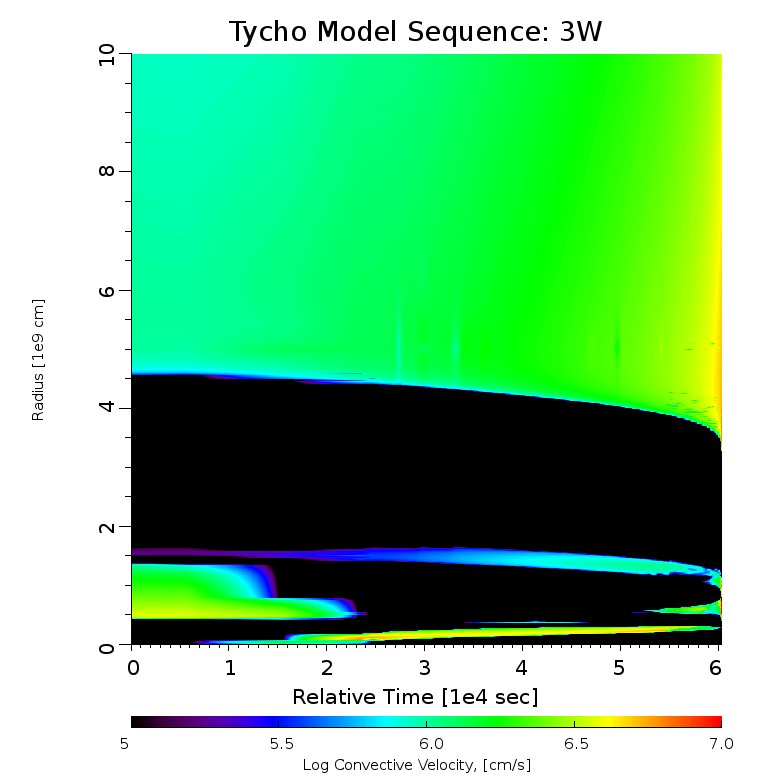
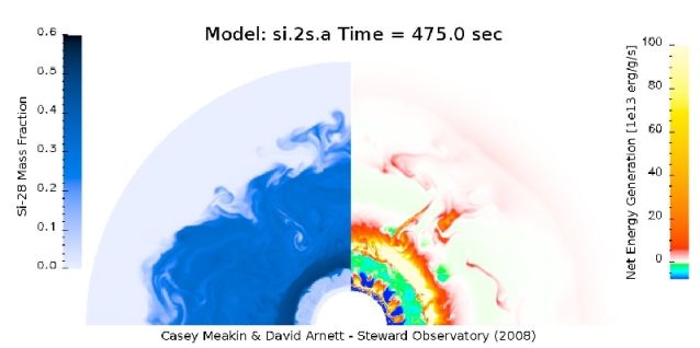
Figure 1: Pre-supernova silicon burning hydrodynamics: (left) The radial dependence of the convective velocity is shown as a function of time for a one-dimensional 23 $\mathcal{M}_{\odot}$ stellar model as it approaches core collapse, which commences at the very end of the time-sequence shown. The innermost convection zone is due to silicon burning, and a transition from core to shell burning can be seen. The overlying convection zones are driven by oxygen, neon, and carbon burning shells. This model was evolved with the TYCHO stellar evolution code. (right) This snapshot shows the distribution of ²⁸Si and net energy generation for a two dimensional hydrodynamic simulation of the TYCHO model $\sim$1000 s before core collapse. Silicon, oxygen, neon, and carbon are burning in concentric shells progressively further away from the iron-rich core which will soon undergo gravitational collapse. The outer boundary of the oxygen burning convection zone is strongly perturbed by the convective motions which eventually mixes the carbon, neon and oxygen burning shells together prior to core collapse (Meakin 2006b).

We have begun a program of multi-dimensional stellar interior modeling which tackles both the quasi-steady and dynamic evolution. Some preliminary work on simulating the reactive hydrodynamic flow associated with pre-core collapse silicon burning in a shell which surrounds an iron core is described in [Meakin & Arnett(2006)] and [Meakin & Arnett(2007a)] (see Figure 1). An interesting discovery is the strong interaction between the turbulent convection and the intervening stably stratified layers. Stable layers are significantly distorted by the convective motions, allow for coupling between different burning zones through waves excited in the stable layers (wave cavities), and significant amounts of material is entrained from the convective boundaries into the burning zones. These effects lead to large asymmetries as core collapse is approached which could play an important role in seeding instabilities and affecting the outcome of core collapse and the subsequent supernova explosion.

3.2 Quasi-Steady Oxygen Shell Burning

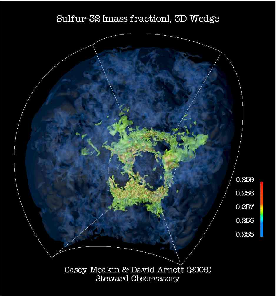
Figure 2: The turbulent flow field in a deep (4 pressure scale height) oxygen burning shell is shown for a computation with a large angular domain (120${}^{\circ}\times 120^{\circ}$), the boundaries of which are shown outlined by white lines. The domain, which is described by spherical polar coordinates, is oriented so that the polar direction is roughly in the up-down direction, and the azimuthal direction is oriented roughly in the left-right direction. The mass fraction of ³²S is visualized in order to give a sense of the topology and the complex, multi-scale, turbulent nature of the flow. Material with a high mass fraction of ³²S is being entrained into the turbulent oxygen burning convective shell from the underlying silicon and sulfur rich core. The computational domain contains 17 million cells. Evolving the flow for 5 convective turnover times requires $\sim$1 million cpu-hours on a computing cluster equipped with quad Intel Xeon EM64T 2.8GHz processor cores. (Data from Meakin & Arnett, 2008 in preparation. )

The neutrino cooled oxygen shell burning epoch is an ideal evolutionary phase to study the physics of quasi-steady state stellar convection. The acceleration of this burning stage due to neutrino cooling reduces the ratio between the thermal and hydrodynamic timescales, hence easing the burden of obtaining a relaxed model (see e.g. [Arnett(1996)], Ch. 10). Recently, we have extended oxygen shell burning simulations to include significantly larger computational domains, longer evolutionary timescales, and 3D flow ([Meakin(2006), Meakin & Arnett(2007b), Meakin & Arnett(2007c)]). A snapshot of the turbulent flow within an oxygen burning shell is presented in Figure 2. While we find a statistically converged, smooth, quasi-steady state, it is characterized on smaller timescales by significant intermittency and fluctuations. This is illustrated in Figure 3, in which we present both a time averaged radial profile and a space-time diagram showing the evolution of the buoyancy work in a convective oxygen burning shell.

4 Processes and Theory

It is important to bear in mind that numerical simulations of stellar convection are not complete and faithful representations of the actual flows present within a stellar interior. What simulation does provide is a fully non-linear solution with a large number of degrees of freedom which is constrained by an ever more realistic astrophysical context (equation of state, background structure and source terms, better nuclear energetics, etc). These solutions provide the theorist with (1) insight into the fundamental processes which might be operating in a stellar interior, and (2) estimates for the amplitudes and length scales present in the flow which drive instabilities on smaller, unresolved scales. The data from these numerical experiments which inspire theoretical ideas, must ultimately be augmented by a richer, and broader theory of basic processes.

4.1 Reynolds Averaged Equations

We develop a kinetic energy (KE) equation in [Meakin & Arnett(2007c)] by decomposing the velocity $\mathbf{u}$, density $\rho$, and pressure $p$ fields into mean and fluctuating components $\varphi=\varphi_{0}+\varphi^{\prime}$, employing the hydrostatic equilibrium condition, and performing averages,

$$\partial_{t}\overline{\langle\rho E_{K}\rangle}+\nabla\cdot\overline{\langle\rho E_{K}\mathbf{u_{0}}\rangle}=-\nabla\cdot\overline{\langle\mathbf{F_{p}}+\mathbf{F_{K}}\rangle}+\overline{\langle p^{\prime}\nabla\cdot\mathbf{u^{\prime}}\rangle}+\overline{\langle\mathbf{W_{b}}\rangle}-\varepsilon_{K}$$ (2)

where $E_{K}$ is the kinetic energy per gram, $\mathbf{W_{b}}$ is the buoyancy work term, $\varepsilon_{K}$ is the viscous dissipation of kinetic energy, $p^{\prime}\nabla\cdot\mathbf{u^{\prime}}$ represents the compressional work done by turbulent fluctuations, and $\mathbf{F_{K}}$ and $\mathbf{F_{p}}$ are kinetic energy and pressure-correlation fluxes. A complimentary equation for the internal energy can may be developed (see [Meakin & Arnett(2007c), Arnett et al.(2008)]).

One of the primary aims in turbulence (and stellar convection) research is to develop physical models for the various terms in these equations, such as the dissipation and flux terms. The reliability of these model terms is only as good as the physical assumptions on which they are based. Often, one is forced to resort to mathematically motivated, ad hoc or phenomenologically based closure models to develop a working theory, and these “theories” are often replete with adjustable parameters which absorb our ignorance about various flow properties. For instance, a commonly used model for the kinetic energy flux is to assume (e.g., [Stellingwerf(1982), Kuhfuss(1986)]),

$$\mathbf{F_{K}}\propto-\nabla(E_{K})$$ (3)

which is sometimes referred to as the down gradient approximation (DGA). Although this model is contradicted by experiment, fundamental theory, and numerical simulation (see e.g., [Pope(2000)]) it remains the cornerstone of many modern turbulence theories which are used in stellar evolution modeling.

One avenue for moving beyond simplified turbulence models and closures such as DGA is to draw upon the physical intuition garnered from (1) ever more realistic numerical simulation, (2) better laboratory flow visualization techniques, and (3) cross pollination between the different fluid dynamics sub-discplines (e.g., oceanography, astrophysics, laboratory combustion, etc).

4.2 Dissipation and the Mixing Length

The dissipation of the piecewise parabolic method (PPM) acts on the smallest scales. The numerical dissipation characteristics of this hydrodynamics algorithm compares remarkably well to other approaches used to model turbulence (see [Benzi et al.(2007), Boris(2007)]). The good energy conservation properties of the finite volume, conservative PPM scheme allows us to infer the dissipation rate of kinetic energy in our convection simulations, which is shown in Figure 4(left). Guided by the dependence of dissipation on the kinetic energy scale of the flow in homogeneous turbulence, we posit that the dissipation in the convective shell can be written as,

$$\varepsilon_{K}=v_{t}^{3}/L$$ (4)

where $v_{t}$ is the rms turbulent velocity fluctuation at a given radius, and $L$ is a “damping length”. Dissipation calculated according to this expression is shown in Figure 4 by the thin line and compares remarkably well to the inferred damping rate, strongly supporting our ansatz about the nature of the dissipation. The damping length $L$, which represents the largest eddy in the system, is comparable to the depth of the convective shell. Solar surface convection simulations (R.Stein, private communication) also show this type of dissipation, though the dissipation length $L$ is about four pressure scale heights and not the entire depth of the convection zone, but still significantly larger than a pressure scale height.

In [Arnett et al.(2008)] we consider the implications that this form of dissipation has for the mixing length theory (MLT) of convection. In particular, we show that if the dissipation length $L$ scales with the depth of the convection zone, the near balance between dissipation and buoyancy driving,

$$\overline{\langle\rho^{\prime}gv_{t}\rangle}=\varepsilon_{K}\approx v_{t}^{3}/L$$ (5)

implies that the mixing length parameter $\alpha$ is a function of the depth of the convection zone,

$$\alpha^{2}\propto L/H_{p}.$$ (6)

While this result depends on various measured properties of the specific flow at hand (such as the correlation coefficient between temperature and velocity fluctuations, $\alpha_{E}=\langle T^{\prime}v^{\prime}\rangle/(T^{\prime}_{\rm rms}v^{\prime}_{\rm rms})$) comparing a wide range of diverse simulations suggest some universality (e.g., $\alpha_{E}\approx 0.7$ for a both oxygen shell burning, solar surface, and ideal box convection simulations; see [Meakin & Arnett(2007c), Arnett et al.(2008)]). That $\alpha$ is not a universal constant appears to be a robust result.

4.3 Entrainment and Buoyancy Flux

The interaction of a turbulent convective region with a bounding stably stratified layer is a long standing challenge to stellar interior modelers. Various phenomenological models have been formulated to treat the mixing that takes place at this interface, but can generally be classified as either (1) a ballistic picture in which eddies penetrate the stable layers until buoyancy breaking halts their motions ([Zahn(1991)]); (2) a diffusive type process operating within the stable layers which mixes material from the convection zone into the surroundings; or (3) an instantaneous mixing in a region of a fixed, parametrized size. While these prescriptions for mixing have been able to solve various astrophysical quandaries (such as cluster color-magnitude diagram fitting), they are not based on robust, self-consistent physical models and contain parameters which are not grounded in more basic physical considerations and must be calibrated. The universality of these parameters is therefore under question, and like the $\alpha$ in MLT are likely not universal constants.

A more detailed and rigorous analysis of the dynamics taking place at a turbulent boundary layer has been considered by both the geophysical and laboratory fluid dynamics communities, and much progress has been made in elucidating fundamental processes which mediate the mixing rates at these boundaries. One of the primary indicators of boundary layer dynamics is the bulk Richardson number ([Fernando(1991)]),

$$Ri_{B}=\frac{bL}{v_{t}^{2}}$$ (7)

for buoyancy jump $b$, outer scale $L$, and rms turbulent velocity $v_{t}$. For large values of $Ri_{B}$, the boundary layers are strongly stratified compared to the strength of the turbulence and mixing proceeds slowly and the boundary remains relatively undistorted. Boundaries with small values of $Ri_{B}$ are strongly distorted by the turbulence, which is attended by more rapid mixing rates. Entrainment rates, defined as a boundary layer migration speed $u$ normalized by the rms turbulent velocity scale, is often found to be well characterized by a simple power law dependence “entrainment law”,

$$E=\frac{u}{v_{t}}=ARi_{B}^{-n}$$ (8)

where A and n are constants fitted to experimental and simulation data. These observations are connected to the underlying hydrodynamic processes through the buoyancy evolution of the boundary layers (see e.g., §7 in [Meakin & Arnett(2007c)]). An interesting result is that this same power law dependence also holds for the astrophysical convection simulations analyzed in [Meakin & Arnett(2007c)] (see right panel in Figure 4).

The evolution of buoyancy is related to the “buoyancy flux” through,

$$\partial_{t}b=-\nabla(q)$$ (9)

where $q=\rho^{\prime}v^{\prime}g/\rho_{0}$ which is related to the buoyancy work term in the Reynolds averaged KE equation above by $q=\rho_{0}\mathbf{W_{b}}$. This conservation law for buoyancy describes the exchange between the kinetic energy in turbulence and the potential energy of stratification. A fundamental theory of mixing at convective boundaries will model these terms (some progress is being made; see [Fernando & Hunt(1997), McGrath et al.(1997)]). While the time and horizontally averaged profiles of the buoyancy flux is smooth, a spatio-temporal decomposition reveals that the smooth profile arises from a highly dynamic underlying behavior (Figure 3).

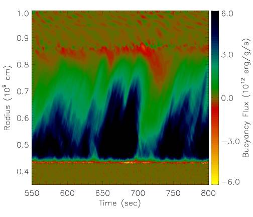
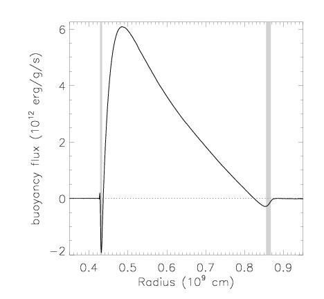
Figure 3: Buoyancy flux. (left) Time-series diagrams and (right) time-averaged radial profiles are shown for 3D oxygen shell burning model described in [Meakin & Arnett(2007c)].

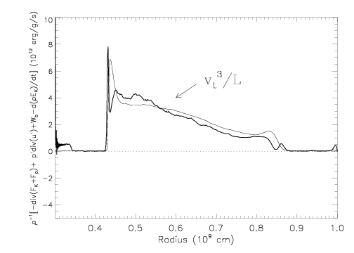
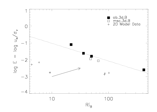
Figure 4: Derived flow properties for a numerical simulation of turbulent oxygen shell burning in a 23 $\mathcal{M}_{\odot}$ stellar model. (left) The inferred turbulent kinetic energy dissipation rate (thick line) is compared to a dissipation rate calculated using the local rms turbulent velocity $v_{t}$ according to $\varepsilon_{K}=v_{t}^{3}/L$ with “damping length” $L$. The rms turublence velocity is based on the velocity variance across the horizontal plane and two convective turnover times for a fixed radius. The damping length represents the largest eddy in the simulation, which is found to be comparable to the depth of the convection zone in this model. (right) The normalized entrainment rate (boundary layer migration rate in units of the rms turbulence velocity at the boundary) is plotted against the bulk Richardson number, $Ri_{B}$. The dashed line shows the best-fit power law to the 3D data. The 2D entrainment rates fall everywhere below the 3D trend due to the incompatible turbulence mixing properties between 2D and 3D flow (see [Meakin & Arnett(2007c)]).