AMBER closure and differential phases: accuracy and calibration with a Beam Commutation

Abstract

The first astrophysical results of the VLTI focal instrument AMBER have shown the importance of the differential and closure phase measures, which are supposed to be much less sensitive to atmospheric and instrumental biases than the absolute visibility. However there are artifacts limiting the accuracy of these measures which can be substantially overcome by a specific calibration technique called Beam Commutation. This paper reports the observed accuracies on AMBER/VLTI phases in different modes, discusses some of the instrumental biases and shows the accuracy gain provided by Beam Commutation on the Differential Phase as well as on the Closure Phase.

1 Introduction

In Optical long baseline interferometry, the phase of the object complex visibility is lost because of the random and fast phase variations introduced by the atmosphere.Three main techniques exist to overcome this strong limitation and recover a part of the phase information: phase referencing[1], where an off axis source in the isoplanetic angle is used as a phase reference, closure phase[2, 3], which is a combination of the phases from three telescopes and is by nature free of any disturbance introduced in any of the beams, and then differential phase[4, 5], which is the same as phase referencing but with the source itself in some particular wavelength as a phase reference.

The phase referencing technique is affected by atmospheric effects, such as chromatic optical path difference (OPD), which is not exactly the same for the reference and the science target. Instrumental effects also affect the phase. Phase referencing technique uses a high precision metrology and a technique of commutation between the science star and the off axis star to overcome these effects. The OPD effects completely disappear in the phase closure, which explain why this phase-measurement technique has been used up to now with great success. However, for high dynamic and high precision measurements, closure phase remains sensitive to all non-OPD instrumental effects. The differential phase is affected by the same effects as the phase referencing technique. The instrumental effects can be reduced by a careful instrumental design, making the conditions of measure of all spectral channels (for example) as identical as possible, but they are almost impossible to eliminate completely. Therefore, a commutation technique would allow one, just like for phase referencing, to overcome in great part the instrumental effects.

To calibrate the differential and closure phases of AMBER, we installed a specific tool called the Beam Commutation Device (BCD). It has been inspired by our experience in differential speckle interferometry (Cuevas and Petrov, 1994) [6] and consists in commuting two of the input beams without otherwise modifying the images pupils positions and OPD values seen by the instrument. The main advantage of such a commutation is that it can be performed very rapidly, to the contrary of usual calibration techniques.

This paper presents a first set of tests of this calibration method on the AMBER instrument and compares it results with those of a standard calibration using a reference star observed at a different time than the science source.

2 AMBER phases and Beam Commutation

We first remind the definitions of differential and closure phase, then discuss their possible biases, the standard calibration procedure, using a reference star and the BCD calibration procedure.

2.1 Differential phase and Closure phase measures and perturbations

2.1.1 The differential phase

In optical, as well as in radio astronomy, source phase information refers to the phase of its complex visibility $\mu$. In a single-mode interferogram, the phase is related to the position of the fringes, and in the absence of nanometer accuracy metrology, the measured phase $\phi_{12}^{m}(\lambda)$ is affected by an unknown instrumental term linked to the VLTI and AMBER differential piston $\delta_{12}(t)$ and to the instantaneous atmospheric piston $p_{12}(t)$ between beams $1$ and $2$, as a function of the wave number $\sigma=1/\lambda$:

$$\phi^{m}_{12}(t,\sigma)=\phi^{*}_{12}(\sigma)+2\pi\left[\delta_{12}(t)+p_{12}(t)\right]\sigma$$ (1)

At this point, we can introduce a development of the source phase $\phi_{12}^{*}(\sigma)$ that will be used afterwards:

$$\phi_{12}^{*}(\sigma)=a^{*}_{0}+a^{*}_{1}\sigma+\delta\varphi_{12}^{*}(\sigma)$$ (2)

where $\delta\varphi_{12}^{*}(\sigma)$ stands for the object phase that cannot be explained by a phase slope as a function of wave number. It contains higher-order terms of the phase polynomial development that are the source information which can be extracted from differential phase measurements.

To compute the differential phase in practice, we use the so-called complex coherent flux, which is usually the rawest measure an interferometer outputs. It contains the instantaneous complex visibility $\mu$, the instantaneous flux $f$, and an additional term $T$ that we call “transfer function” which contains all the atmospheric and instrumental effects on the complex visibility:

$$C^{m}_{12}(t,\sigma)=F(t,\sigma)T(t,\sigma)\mu(\sigma)$$ (3)

The phase of the transfer function term $T$ contains the terms $\delta_{12}(t)$ and $p_{12}(t)$ described before, and the phase of $\mu$ contains the object phase $\phi_{12}^{*}(\sigma)$. The differential phase is obtained in practice by fitting the measured phase $\phi^{m}_{12}(t,\sigma)$ with a linear function $\varphi^{\rm fit}_{12}$ of $\sigma$, therefore enclosing the terms $\delta_{12}$, $p_{12}$, $a^{*}_{0}$ and $a^{*}_{1}$:

$$\varphi^{\rm fit}_{12}(t,\sigma)=2\pi(\delta_{12}(t)+p_{12}(t)+a^{*}_{1})\sigma+a^{*}_{0}$$ (4)

We correct then $C^{m}_{12}(t,\sigma)$ from this effect on a frame-by-frame basis, obtaining $C^{nop}_{12}(\sigma_{i})$, and we integrate it in a reference channel, obtaining $C^{\rm ref}_{12}(t,\sigma_{i})$:

$$C^{\rm nop}_{12}(t,\sigma_{i}) = C^{m}_{12}(t,\sigma_{i})e^{-i\varphi^{\rm fit}_{12}(\sigma_{i})}$$ (5)

$$C^{\rm ref}_{12}(t,\sigma_{i}) = \sum_{j\neq i}^{n_{\sigma}}C^{m}_{12}(t,\sigma_{j})e^{-i\varphi^{\rm fit}_{12}(t,\sigma_{j})}$$ (6)

The differential phase is then computed by:

$$\delta\phi^{m}_{12}(\sigma)=arg\left[<C^{\rm nop}_{12}(t,\sigma)\times\left(C^{\rm ref}_{12}(t,\sigma)\right)^{*}>_{t}\right]$$ (7)

Therefore, in the way it is defined, this differential phase is an estimator of the beforehand mentioned (eq. 2) high order term of the object phase:

$$\delta\phi^{m}_{12}(\sigma)\equiv\delta\varphi_{12}^{*}(\sigma)$$ (8)

2.1.2 The effects affecting the differential phase

The measured differential phase is affected by the source phase $\delta\varphi^{*}_{12}(\sigma)$, the atmosphere chromatic phase $\delta\phi^{a}_{12}(\sigma)$, and the instrument chromatic phase $\delta\phi^{i}_{12}(\sigma)$. It can be expressed as:

$$\delta\phi^{m}_{12}(\sigma)=\delta\varphi^{*}_{12}(\sigma)+\delta\phi^{a}_{12}(\sigma)+\delta\phi^{i}_{12}(\sigma)$$ (9)

The term $\delta\phi^{a}_{12}(\sigma)$ results only from a chromatic OPD term as the rapidly variable achromatic term is removed during the fitting process (eq. 4). This effect is supposed afterwards to have slow variations with time. The term $\delta\phi^{i}_{12}(\sigma)$ contains only the chromatic instrumental effects, for the same reasons as before. The main effects affecting the AMBER differential phase are described briefly in the following list:

• The atmospheric chromatic effect comes mainly from the different thickness of dry and wet air in each beam. Since the refraction index of the gases is wavelength dependant, this result in a chromatic OPD. A first order correction is made from computed gas indexes and known delay line positions, but short term variations of temperature, pressure and humidity leave phase terms which vary of several hundreds of radians. This effect is linked to dry air and water vapour content and is explained in details in Mathar et al.[7]. At $2\mu$m, in the AMBER data, this effect is seen as a global curvature of the differential phase relative to wavelength that can have amplitudes of up to 1 rad.

• The dichroics contained in AMBER, due to reflexions and refractions, produce a chromatic phase bias seen mainly at the beginning of the K band (1.95$\mu$m) and which seems to be stable with time.

• The detector gain table change with time (or the change of the pixels used to read the interferogram) produce in first approximation and additive effect on the differential phase, which can be different from any spectral channel (i.e. lines of pixels). This results in a noise of the differential phase as a function of wavelength, that might be overcome if the time-variations of this $\lambda$-noise are slow enough

• There are variable modulations in wavelength in the measured spectra, visibility, differential phase and closure phase. There are some time nicknamed “socks”. We first suspected the optical fibers to be imperfect spatial filters. It has been recently shown that any plane parallel plate introduced in the beam actually produces a Perot-Fabry effect, with a mixing of waves directly transmitted and of one or several waves who have crossed the plate $2n$ more times. The most recent measures [8], show that the strongest effect, by far, results from the AMBER polarizers put in each beam. The effect change with temperature and mechanical excitation and result in the variation described below. These polarizers will be replaced soon, but this paper shows how the BCD cope with these modulations in the differential phases so far.

2.1.3 The closure phase

The closure phase between baselines $\overrightarrow{B_{12}}$, $\overrightarrow{B_{23}}$ and $\overrightarrow{B_{31}}$ is the phase of the average ”bi-spectral product” of the coherent fluxes:

$$\psi_{123}=arg\left[<C^{m}_{12}\,C^{m}_{23}\,(C^{m}_{31})^{*}>_{t}\right]$$ (10)

and it is a very classical property of long-baseline interferometry that this closure phase is independent of any OPD terms affecting individually each beam. This includes the achromatic OPD, as well as the chromatic one:

$$\psi_{123}=\phi^{*}_{12}+\phi^{*}_{23}-\phi^{*}_{13}+\phi^{d}_{12}+\phi^{d}_{23}-\phi^{d}_{13}$$ (11)

where $\phi^{d}_{ij}$ are error terms linked to the baseline $ij$, due for example to a change in the detector gain table between the flat field evaluation and the observation.

2.1.4 The effects affecting the closure phase

By construction the closure phase if free from any path difference introduced in any individual beam. However it is sensitive to detection effect related to each baseline:

• If the pixels (or their gain) used to analyze a spectral channel have changed since the instrument calibration, all phases will be modified in a way which depends from the baseline interferogram calibration and not to the OPD and does not have any reason to produce null closure phases. It will appear, as in the case of differential phase, as a $\lambda$-noise, that hopefully does not vary rapidly with time.

• The situation with the wavelength beatings and the spatial filtering defects are unclear at this point. They introduce phase differences in each beam (which should be canceled out in the closure phase) but also in each interferogram fit and the latest should produce a non zero closure phase as seen below in the measures.

2.2 Calibrating the phases with a reference star

2.2.1 Calibrating the differential phases

Calibration of the differential phase is the removal of all the instrumental and atmospheric effects from the phase signal described in Sect. 2.1.2. The calibrated differential phase is thus:

$$\delta\phi^{c}_{12}(\sigma)=\delta\phi^{m}_{12}(\sigma)-\widehat{\delta\phi}^{a}_{12}(\sigma)+\widehat{\delta\phi}^{i}_{12}(\sigma)$$ (12)

where $\widehat{\delta\phi}^{a}_{12}(\sigma)$ and $\widehat{\delta\phi}^{i}_{12}(\sigma)$ are estimations of the atmosphere and instrumental differential phases. A way of estimating these terms is to observe a centro-symmetric star whose phase $\widehat{\delta\phi}^{*c}_{12}(\sigma)$ is known to be zero at all wavelengths. The calibrated differential phase is then:

$$\delta\phi^{c}_{12}(\sigma)=\delta\phi^{m}_{12}(\sigma)-\delta\phi^{*c}_{12}(\sigma)$$ (13)

However, one can see that the calibration must be rapid enough to consider that the calibration star differential phase $\delta\phi^{*c}_{12}(\sigma)$ is equal to the differential phase $\widehat{\delta\phi}^{a}_{12}(\sigma)+\widehat{\delta\phi}^{i}_{12}(\sigma)$ we want to remove from the science star. Also, a very similar air mass should be used between the science star and the calibration star in order to avoid large changes in the term $\delta\phi^{a}_{12}(\sigma)$. In practice, at VLTI, the calibration cycle is at least 30 mn, where the atmospheric water vapour content has enough time to change by large amounts. Also, in 30 mn, the instrument has enough time to move as the focal laboratory temperature slightly changes with time.

2.2.2 Calibrating the closure phase

For the closure phase terms linked to a drift of the instrument calibration, the same technique and restriction applies. They can be cancelled by the use of a reference star if they are stable other the 20 to 30 mn time necessary to switch from science to reference.

2.3 Calibrating the phases with beam commutation

The beam commutation, as briefly explained in introduction, is meant to remove a part of the phases artifacts presented in Sect. 2.1.2. It can be fully seen as an alternative calibration technique to the standard science-reference stars presented in Sect. 2.2. Indeed, the instrumental phase effects can be considered stable over a given time span. In AMBER, for example, the described dichroic phase effect and the detector gain table are stable over several minutes.

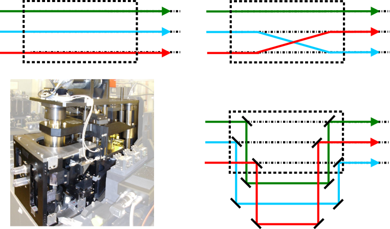
Figure 1: The beam commutation explained in few sketches: Top-left: the standard scheme where the beams go through unaffected in the instrument. Top-right: The Beam Commuting Device is inserted in the beam and switches two out of the three beams. Bottom-left: A photo from the authors of the AMBER BCD, as it has been build, with 6 additional specular reflexions per beam. Bottom-right: A simplified sketch of how the AMBER BCD commutes the beams. One needs 6 reflexions on flat mirrors to keep both the pupil and the image at the same position as well as the same OPD.

2.3.1 Calibrating the differential phases by beam commutation

Let us consider that at some point of the interferometer, one can swap beams 1 and 2 in a specific device called Beam Commuting Device (hereafter called BCD, see Fig. 1). The phase $\delta\varphi_{12}^{*}(\sigma)+\delta\phi^{a}_{12}(\sigma)$, before the BCD, is now recorded as being 21 instead of 12, thus changing its sign compared to the unswapped situation. The phase introduced after the BCD point $\delta\phi^{i}_{12}(\sigma)$, in the instrument, is left unchanged:

No BCD: $$\delta\phi^{m}_{12}(\sigma)= \ \delta\varphi^{*}_{12}(\sigma)+\delta\phi^{a}_{12}(\sigma)+\delta\phi^{i}_{12}(\sigma)$$

With BCD: $$\delta\phi^{m{\rm,BCD}}_{12}(\sigma)= -\delta\varphi^{*}_{12}(\sigma)-\delta\phi^{a}_{12}(\sigma)+\delta\phi^{i}_{12}(\sigma)+\delta\phi^{\rm BCD}_{12}(\sigma)$$ (14)

The idea is then to record data as usual, to perform the beam commutation and then to record commuted data. When subtracting the two measurements, and if the instrument is stable enough (i.e. both the instrumental term and the atmospheric one are stabilized after the BCD), the terms $\delta\phi^{a,{\rm A}}_{12}(\sigma)+\delta\phi^{i,{\rm A}}_{12}(\sigma)$ cancel out:

$$\delta\phi^{c}_{12}(\sigma)=\frac{\delta\phi^{m}_{12}(\sigma)-\delta\phi^{m,BCD}_{12}(\sigma)}{2}=\delta\phi^{*}_{12}(\sigma)+\delta\phi^{a{\rm B}}_{12}(\sigma)+\delta\phi^{i{\rm B}}_{12}(\sigma)$$ (15)

If a beam commuting device is built, it must not affect the beams with more effect on the phases than the photon noise over one calibration cycle, i.e. the term $\delta\phi^{\rm BCD}_{12}(\sigma)$ is smaller than the noise on the phase due to fundamental noises only. One of the main interests of the beam commutation is that it allows shortening the calibration cycle with regard to the use of a natural reference star. For example, on AMBER, we go from about 30 minutes to about 2-3 minutes.

One can also see that, using this technique, the term before the BCD $\delta\phi^{a}_{12}(\sigma)$ cannot be removed. Therefore, one still has to cope with the atmospheric term, which is anyway present also when calibrating with a natural reference star.

2.3.2 Calibration of Closure phase by beam commutation

Closure phase is insensitive to all atmospheric and most instrumental effects, due to the fact that they cancel out in the closure relation. However, the instrumental effects that are after the recombination do affect the closure phase. These effects are in AMBER mainly coming from camera distortion and from detector gain table uncertainty. The Fig. 2 illustrate how the closure phase artifacts get calibrated out by the beam commutation. Therefore, the same ideas apply when using the BCD with closure phase.

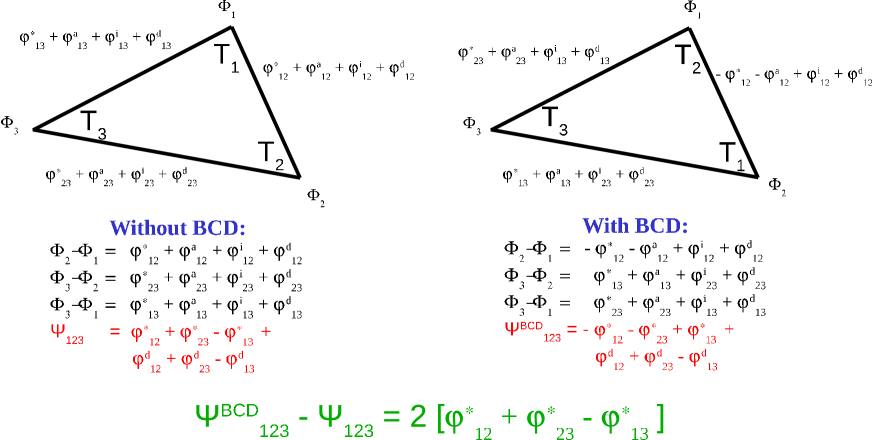
Figure 2: The reason why closure phase can benefit from beam commutation is presented here: the instrumental effects taking place after the combination are cancelled out by subtracting the two closure phases recorded with and without BCD respectively.

3 Experimental results

We describe here measures of differential phase accuracy calibrated both in standard way on a reference star and with the Beam Commuting Device described above. We show and discuss some results in medium resolution and low resolution in the K band (MR-K and LR-K). We also show some very recent closure phase measures obtained on the ATs with FINITO[9], which allowed us for the first time to obtain closure phases good enough for an accuracy discussions. All our objects (but one) are calibrators supposed to yield zero differential and closure phase, mostly obtained during the commissioning with two ATs in July 2006 and during some Guaranteed Time attempts to measure the very small phases and/or closure phases indicating the presence of a planet around Tau Bootis. Please note that in all figures, the values for the wavelength are only indicative. An accurate spectral calibration was not relevant to the problem discussed here and the wavelength scales can have offsets up to 0.1$\mu$m.

3.1 Observations and data processing

We illustrate the different observations and data processing steps on the MR-K data obtained with two ATs in 2006. The data processing has been made with amdlib v2.0. The exposures are processed individually, with the standard data processinf and selection of 20% of best frames.

• In the STD mode, the chromatic OPD is fitted through and subtracted from the science and calibrator differential phases separately. Then, the calibrator differential phase is subtracted from the science one, yielding a calibrated differential phase.

• In the SPA mode, we compute the half difference between the differential phases obtained on BCD-out and BCD-in exposures. Then the chromatic OPD is fitted and subtracted yielding the calibrated differential phase.

3.2 Differential phases calibration at medium spectral resolution

The Fig. 3 illustrate the different steps of the standard calibration (left, labeled STD) and the calibration with the BCD (right, labeled SPA, for SPAtial modulation, which as already explained is actually what the BCD is approaching). The target is Achernar (K=0.88, seeing 1.3 arcsec, t0=1.7 ms), and the calibrator is HD 219215 (K=0.1, seeing 1.5 arcsec). In spite of the fast seeing, the data was acquired with single exposure time of 160 ms, allowing to have full K Band spectral window and more clear results. The measured spectra is underlying in each figure. All figures show the source + AMBER spectra in a fin grey line. The spectral calibration has not been made with care since it does not affect the measurements, and there is about 0.1$\mu$m offset in the wavelength labels. However, the spectra of science and calibrators have been very carefully corrected for any relative offset.

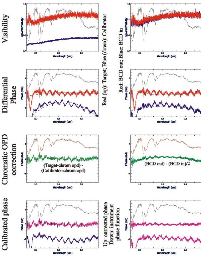
Figure 3: These plots show the comparison of standard calibration with a natural star (left column, STD) with the beam commutation calibration (right column, SPA stands for “SPAtial modulation”). The top line shows the visibilities. One can see that the BCD does not affect the visibility measurement on the star (right column). Only the error bars are slightly larger to a flux loss of about 20-50% (depending on how the BCD is aligned). The second line shows the raw differential phases for the star and the calibration star in the left part and for BCD-in and BCD-out for the right part. One can see the many effects affecting the differential phases, ranging from dichroic chromatic effects, “socks” and atmospheric longitudinal chromatic dispersion. Third line shows the “calibrated” differential phase (i.e. the difference of the two previous ones). One can see here the remaining artifacts: mainly atmospheric dispersion and “socks” residuals. The bottom line compares the final product, where the atmospheric dispersion was removed by fitting a 2nd order polynomial to the phase with the sum of the phases in the 2nd line, giving an indication of the instrumental-only effects.

• Visibility: the two upper figures show the absolute visibility of the source (red) and of the calibrator (blue). Note that in the SDT mode the calibrator is quite resolved but much brighter than the source, explaining the much smaller error bars. In the SPA mode, the red curve stands for BCD-out and the blue for BCD-in. We see that the BCD does not affect the absolute visibility value nor accuracy.

• Differential phase: the second line of figures show the differential phases (red: science or BCD-out; blue: calibrator or BCD-in). The underlying dashed curve is a fit of the chromatic OPD. There are several stringent features.

  • The differential phase is affected by biases larger than the fundamental noise represented by the error.

  • At 1.95$\mu$m we see a strong phase distortion, larger than 1 radian, and due to the K band dichroic.

  • There is a 0.3 radians modulation of the differential phase with a period of about 0.02$\mu$m.

  • The chromatic OPD is the same with the BCD-in and the BCD-out, but for its sign, while it is substantially different for the science and the calibrator.

• In the third line of figures we see the result of the BCD calibration at the right. Normally we should be left only with the chromatic OPD, which is indeed dominating the figure, and with stellar structures if any. Actually there is a clear signature of ”rotating disk type” at the $Br_{\gamma}$ position (the source was the bright Be star Achernar). However, we see that the wavelength modulation has been very strongly reduced but not completely canceled. This means that the wavelength modulation is partially evolving faster than the 60 seconds BCD calibration cycle.

• Chromatic OPD: The BCD calibrated phase is clearly dominated by the chromatic OPD, which allows a clean fit of this feature. Then a final subtraction yields the fully calibrated differential phase in the lower right figure (green line). In the STD mode, the instrumental features corrupt the chromatic OPD fit and there is a clear chromatic OPD residual in the calibrated data.

• Calibrated differential phase: the lower line of figures show the differential phases calibrated by the standard method (left) and by the BCD method (right). The latest is clearly superior, although not perfect.

  • The residual of wavelength modulation are stronger and less periodic in the STD calibration. This indicates that the modulation variation is substantially larger other the much longer standard calibration cycle.

  • The STD calibrated curve is contaminated by a chromatic OPD residual

  • The STD calibrated curve shows in addition to the wavelength modulation many spikes and an apparently much larger noise. This cannot be noise, since we see that the raw calibrator differential phase is much less noisy, in terms of fundamental noise indicated by the error bars, than the BCD-in phase. This shows that the BCD eliminates artifacts that are currently dominated by the wavelength modulation but which will be dominant when the polarizer are replaced.

In this work, Achernar was expected to behave as a bright calibrator (previous, standard, observations failed to detect a feature in the $Br_{\gamma}$ line) and we were quite surprised to see a clear disk signature in the SPA calibrated data. The same features actually exists in the STD differential phase but would be impossible to believe.

The table 1 shows a more quantitative analysis of this data. We see that the SPA calibration gets much closer to the fundamental noise $\sigma$ due to photon, detector and background noise. More important the peak to valley features in wavelength are reduced by almost a factor 3 and are much more regular in SPA mode, allowing further fits in the continuum to be extrapolated in the line.

However, the BCD does not allow to cancel completely the wavelength modulation, which still prevents us reaching our highest goals in differential phase accuracy.

The available data in MR-K does not allow to conclude about the ultimate phase accuracy, since we were already too close to the fundamental noise of about 0.03 radians, but it seems clear that going much better in MR-K (with FINITO for example) for science applications such as Doppler imaging or asteroseismology would have to wait and hardware correction of the main source(s) of wavelength modulation.

Table 1: Table presenting the main comparison between the standard (STD) and beam-commuted (SPA) calibrations. The raw phases show typical patterns of 0.1-0. radians amplitude, due to the chromatic air dispersion as well as the “socks” and the instrumental chromatic effects. The standard calibration diminishes these $\lambda$-patterns basically to 3/2 of the fundamental noise ($\sigma$ column), whereas the beam-commutation allow to reach the fundamental noises.

$\sigma$	PTV ($\lambda$)	RMS ($\lambda$)	Comment
Averaged phases
0.033	0.34	0.172	Achernar (BCD in)
0.035	0.35	0.173	Achernar (BCD out)
0.025	0.34	0.294	Calibrator (HD219215)
Calibrated phases
0.041	0.29	0.069	STD
0.048	0.12	0.044	SPA

3.3 Differential phase calibration in low spectral resolution

Another set of data shows the effect of the BCD calibration with observations made in low spectral resolution ($R=35$). The results appearing in Fig. 4 illustrate the effect of the BCD calibration: after subtraction of the chromatic dispersion fit, the calibrated phase is flattened and smoothed from instrumental artifacts.

Table 2 allows to compare the BCD calibration with the standard calibration, consisting in making the difference Target - Calibrator.

The key result is that the STD calibration leave PTV wavelength features larger than 0.15 radians, corresponding to the variation of the LR instrumental differential phase in one hour, while the SPA calibration reduces the PTV features in lambda below the statistical RMS between frames in a given spectral channel, which we used to consider as a good estimate of the fundamental noise. With this limited set of poor quality data it is possible to conclude that the SPA mode allows to reach a differential phase accuracy better than 0.01 radians.

This measure was also intended to check if calibration combining SPA calibrated differential phases from a source and a calibrator could allow further progress, for example by removing systematic effects introduced by the BCD, but this tests results impossible since both calibrators are cleaned below the fundamental noise limit.

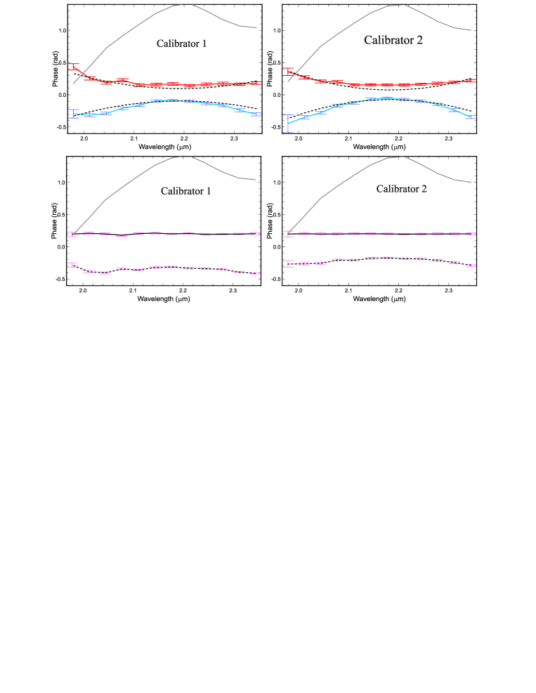
Figure 4: Differential phases using the BCD, for two calibrators observed one hour apart . In each plot, the upper thin black curve represents the spectrum. In the upper plots, the red and blue curves represent the differential phases observed, respectively, with and without the BCD. In their half-sum, the instrumental effects are in principle removed and only the chromatic OPD effects should remain. These have been approximated using a polynomial fit, which is represented by the thin black curves superimposed on the differential phases curves in the upper plot. The lower plots show the half-differences (solid line) and half-sum (dashed line) of these curves, after subtraction of the chromatic OPD fit. Note that the BCD-calibrated phase, which appears in the half-difference (BCD out - BCD in)/2, is indeed very much flatter and smoother than the phase observed without BCD.

Table 2: Summary of the statistics on the differential phase for a science source and its calibrator, in different observation and calibration modes: for BCD OUT and IN, and for a calibration using the BCD (phase OUT - phase IN)/2 or using the standard Target-Calibrator comparison. In each case, we indicate the statistical RMS (averaged over $\lambda$) between the exposures, and the Peak-to-Valley (PTV) and RMS over $\lambda$ of the averaged phase. For the latter two quantities, the polynomial fit of the chromatic dispersion, estimated for the average BCD-calibrated phase, was previously subtracted in the same way as presented in Fig. 3.

Source and	Statistical RMS	PTV over $\lambda$	RMS over $\lambda$
calibration mode	between exposures
Calibrator 1 (OUT)	0.011	0.15	0.0288
Calibrator 1 (IN)	0.018	0.15	0.027
Calibrator 2 (OUT)	0.015	0.10	0.027
Calibrator 2 (IN)	0.019	0.10	0.026
Cal 1 - Cal 2 (STD)	0.012	0.15	0.011
Calibrator 1 (SPA)	0.017	0.01	0.002
Calibrator 2 (SPA)	0.013	0.03	0.009

3.4 Closure phase calibration in low spectral resolution

The principle of closure phase calibration using the Beam Commutation Device, described in Sec. 2.3.2, is illustrated in Fig. 5. This is the result of some recent observations made in low spectral resolution with FINITO, which gave us for the first time high quality closure phases. We had, for calibrators presented here, a series of 10 or 15 exposure pairs, each of them containing an observation with and without the BCD. The half-difference of the closure phase within each pair should in principle be corrected from all the OPD effects affecting each beam, and from the post BCD instrumental effects if these are stable over the BCD cycle period. We find that the BCD corrects the general closure phase bias, smooths channel to channel closure phase features but remains affected by small time variable effects which can be the LR aspect of the wavelength modulation on the closure phase.

• The raw closure phases, both with and without the BCD, are globally offset by about 0.15 radians. This is probably due to the obsolescence of the instrument calibration, made about three hours before the first observation, even if the offset change by much less than 0.1 radians during the three hours separating the two displayed observations. The BCD calibration brings the average closure phase between 0.01 and 0.02.

• The closure phases show features in each spectral channels, which are partially stable in pattern but quite variable in amplitude (by about 0.02 radians in 3 hours).

• The BCD calibrated closure phase is much smoother in wavelength, with a PTV of about 0.02 radians and a RMS of about 0.008 radians. This RMS remains substantially larger than the fundamental noise in that case (0.002 radians). So we are limited by the instrument at about 0.01 radians per calibrated observations, at least with the current hardware and software.

As a whole, the BCD-calibrated closure phases look much more to what we would expect from the astrophysical signature of this observable (i.e., in the present case with calibrators, a flat curve at 0). Nevertheless, both the average and the lambda-rms levels of our calibrated closure phases are well above effects due to the fundamental noise. This therefore indicates that the calibration is not complete. The hypothetical causes for this residual may well be some parasite Fabry-Perot interferences within AMBER dioptres and/or some non-mono-mode effect of the spatial filtering, resulting in the “socks” pattern already mentioned in Sec. 3.2.

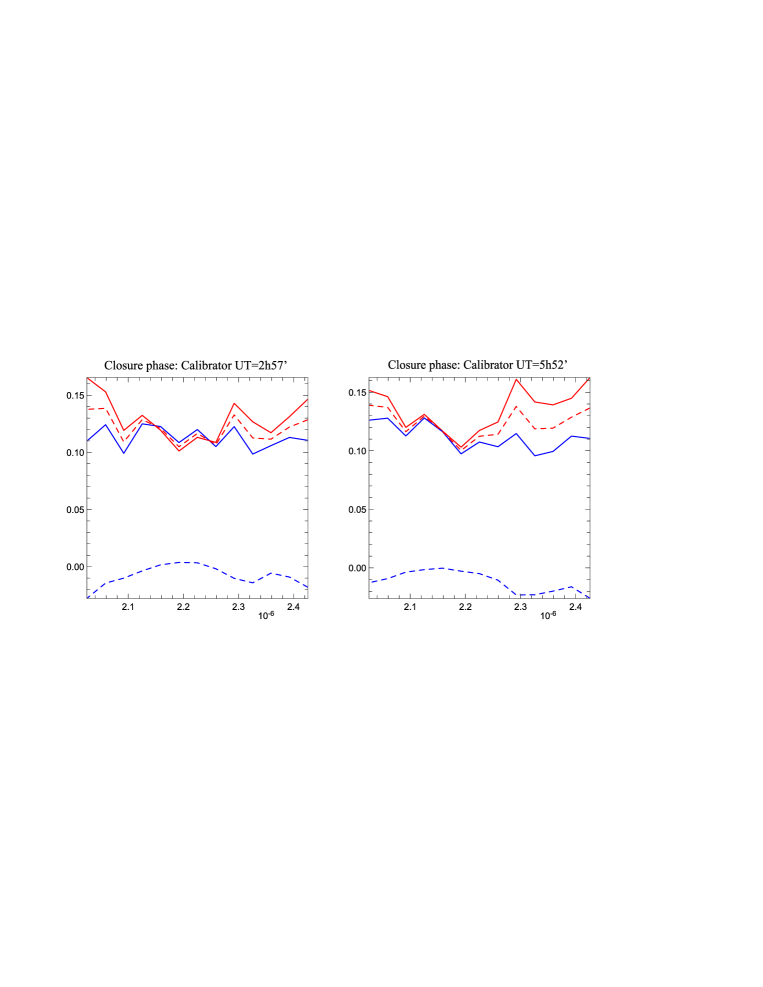
Figure 5: Closure phases observed in Low Resolution with the ATs, using the Beam Commuting Device (BCD), for two calibrators. Full lines refer to averaged exposures without (blue) and with (red) the BCD. The red dashed line is the half-sum of the closure phases (with and without BCD) and represent, in principle, the instrumental contribution to the non-calibrated closure phase. The blue dashed line is the half-difference of the closure phases, where the instrumental contribution should have been corrected by the use of the BCD. We note that these calibrated closure phases are indeed improved, with a lower average level and a smoother shape. But that they still show a significant residual, the theoretically expected closure phase for these targets being a flat null curve.

4 Conclusion

We have shown that the AMBER differential and closure phases display evolving patterns much larger than expected and specified. With a standard calibration using a reference star, it seems difficult to trust phase features smaller than 0.1 radians. This is confirmed by data on other stats and in other bands (MR-H and LR-H) that we could fit in this paper. Since our observations, we have learned that the main perturbation results from Perrot Fabry effects in various glass and air blades, both within AMBER and before it (IRIS feeding dichroic). The major cause for this perturbations has been proved to be the AMBER polarizing filters which will be soon replaced and relocated to minimize this wavelength beating effects.

The specific phase calibration function that we have developed improves the situation but quite not enough. With our Beam Commutation Device we can approach the 0.01 radian limit in the best cases, but this remains much larger than the fundamental noise limits, which are at least 10 times smaller with the ATs and 100 times smaller with the UTs.

The BCD clearly improves other sources of phase errors, more likely to be found in the calibration of the detector or of the position of the beams on the detector. This gives us good hope that the combination of Perrot Fabry effect suppression and of BCD calibration will allow us to approach the 0.001 radians limit, that we already approach in LR-K differential phase.

With the current hardware and without using the BCD, we had 0.1 radian (5 degrees) accuracy on phase, which was enough for the first science application on large disks ($\alpha$ Arae cite) or on binaries with almost equal components ($\gamma^{2}$ Velorum cite). With the BCD and a carefully data processing, we can approach the 0.01 radian specification sufficient for most circumstellar physics (disks and wind in stars of all ages) and by combining hardware and software upgrades with the BCD calibration we still confidently hope that the milliradian limit needed for extra solar planets and stellar activity work will be achieved.

References

- [1] Quirrenbach, A., Coude Du Foresto, V., Daigne, G., Hofmann, K. H., Hofmann, R., Lattanzi, M., Osterbart, R., Le Poole, R. S., Queloz, D., and Vakili, F., “PRIMA: study for a dual-beam instrument for the VLT Interferometer,” in [Astronomical Interferometry ], Reasenberg, R. D., ed., 3350, 807–817, SPIE (July 1998).
- [2] Baldwin, J. E., Haniff, C. A., Mackay, C. D., and Warner, P. J., “Closure phase in high-resolution optical imaging,” Nature 320, 595–597 (Apr. 1986).
- [3] Kraus, S., Schloerb, F. P., Traub, W. A., Carleton, N. P., Lacasse, M., Pearlman, M., Monnier, J. D., Millan-Gabet, R., Berger, J.-P., Haguenauer, P., Perraut, K., Kern, P., Malbet, F., and Labeye, P., “Infrared Imaging of Capella with the IOTA Closure Phase Interferometer,” AJ 130, 246–255 (July 2005).
- [4] Akeson, R. L. and Swain, M. R., “Differential phase mode with the Keck Interferometer,” in [ASP Conf. Ser. 194: Working on the Fringe: Optical and IR Interferometry from Ground and Space ], Unwin, S. and Stachnik, R., eds., 89 (1999).
- [5] Vannier, M., Petrov, R. G., Lopez, B., and Millour, F., “Colour-differential interferometry for the observation of extrasolar planets,” MNRAS 367, 825–837 (Apr. 2006).
- [6] Cuevas, S., Petrov, R. G., Chelli, A., Lagarde, S., Couve, A., Tinoco, S., and Sanchez, L., “Franco-Mexican Differential Speckle Interferometer,” in [Proc. SPIE Vol. 2200, p. 501-511, Amplitude and Intensity Spatial Interferometry II, James B. Breckinridge; Ed. ], Breckinridge, J. B., ed., 501–511 (June 1994).
- [7] Mathar, R. J., “Calculated refractivity of water vapor and moist air in the atmospheric window at 10 m,” Appl. Opt. 43, 928–932 (Feb. 2004).
- [8] A. Chelli and G. Duvert and P. Kern and F. Malbet, “February 2008 ATF run report,” Tech. Rep. VLT-TRE-AMB-15830-7120, AMBER consortium (apr 2008). Issue 1.2 Date : 16/04/2008.
- [9] Le Bouquin, J.-B., Bauvir, B., Haguenauer, P., Schöller, M., Rantakyrö, F., and Menardi, S., “First result with AMBER+FINITO on the VLTI: the high-precision angular diameter of V3879 Sagittarii,” A&A 481, 553–557 (Apr. 2008).