Site Dilution in the Half-Filled One-Band Hubbard Model: Ring Exchange, Charge Fluctuations and Application to La₂Cu_1-x(Mg/Zn)_xO₄

Abstract

We study the ground state quantum spin fluctuations around the Néel ordered state for the one-band ($t,U$) Hubbard model on a site-diluted square lattice. An effective spin Hamiltonian, $H_{\rm s}^{(4)}$, is generated using the canonical transformation method, expanding to order $t(t/U)^{3}$. $H_{\rm s}^{(4)}$ contains four-spin ring exchange terms as well as second and third neighbor bilinear spin-spin interactions. Transverse spin fluctuations are calculated to order $1/S$ using a numerical real space algorithm first introduced by Walker and Walsteadt. Additional quantum charge fluctuations appear to this order in $t/U$, coming from electronic hopping and virtual excitations to doubly occupied sites. The ground state staggered magnetization on the percolating cluster decreases with site dilution $x$, vanishing very close to the percolation threshold. We compare our results in the Heisenberg limit, $t/U\rightarrow 0$, with quantum Monte Carlo (QMC) results on the same model and confirm the existence of a systematic $x$-dependent difference between $1/S$ and QMC results away from $x=0$. For finite $t/U$, we show that the effects of both the ring exchange and charge fluctuations die away rapidly with increasing $t/U$. We use our finite $t/U$ results to make a comparison with results from experiments on La₂Cu_1-x(Mg/Zn)_xO₄.

I Introduction

I.1 Random disordered magnets

Magnetic materials and model magnetic systems are perhaps the best test benches for the study of collective phenomena in nature. This is particularly true in the context of systems with frozen or quenched random disorder Grinstein (1985); Ill (1979). Here, questions such as the sharpness of phase transitions in disordered systems Harris (1974), the stability of ground-state symmetry-breaking (random-field) perturbations Imry and Ma (1975) and spin glass behavior arising from random frustration Binder and Young (1986) have come under sharp scrutiny over the past thirty years.

The 1987 discovery of high-temperature superconductivity in doped antiferromagnetic copper oxide materials generated a huge amount of interest in quantum antiferromagnets which continues to this day Anderson (1987); Sachdev (2008). Here, the magnetic properties depend strongly on the different possible types of quenched disorder and this has proven to be a rich source of novel quantum phenomena. An important area of investigation has been to explore how the ground state of insulating quantum magnets evolves as the level of random disorder is changed. The following examples represent a small subset of this class of studies. A large effort has been targeted towards understanding the properties of antiferromagnetic spins chains subject to various types of disorder Shender and Kivelson (1991); Eggert and Affleck (2004); Sirker et al. (2008). Further work investigated how long range order develops in two and three dimensional arrays of weakly coupled integer (Haldane) spin chains Shender and Kivelson (1991) and even-leg ladders Azuma et al. (1997). The question of how Néel order develops upon magnetically diluting pure systems with quantum spin liquid ground states is another field of intensive study Wessel et al. (2001).

Theoretical problems relating to various types of random bond disorder, as opposed to the more material-relevant case of site dilution, have also been investigated Sandvik and Vekic (1995); Yu et al. (2006). In three dimensional systems, one noteworthy example is the so-called antiglass phenomenon in LiHo_xY_1-xF₄ where, for a low concentration, $x$, of magnetic Ho³⁺ ions, the dipolar spin glass phase seemingly disappears Ghosh et al. (2003). Another interesting problem concerns the role frozen random impurities may play at conventional and deconfined quantum critical points in two-dimensional antiferromagnets Metlitski and Sachdev (2007).

However, among the multitude of interesting problems, a particular one, possibly because of its seemingly simple physical setting and its broad conceptual appeal, has drawn considerable attention: that of the evolution of the antiferromagnetic Néel ground state in the site-diluted $S=1/2$ nearest neighbor square lattice Heisenberg antiferromagnet (SLHAF).

I.2 Site-diluted SLHAF and La₂Cu_1-x(Mg/Zn)_xO₄

As the insulating and antiferromagnetic parent of high-temperature superconductivity in La_2-xSr_xCuO₄, La₂CuO₄ has quasi two dimensional magnetic exchange interactions and a good starting point for its description is to treat the CuO₂ planes as decoupled SLHAFs. Hence, experimental studies on zinc and magnesium substitution for copper in La₂CuO₄ Chakraborty et al. (1989); Cheong et al. (1991), provided some of the earliest motivation and interest in the problem of site-diluted SLHAFs Wan et al. (1991). In particular, Cheong et al. Cheong et al. (1991) found from bulk thermodynamic measurements that in the diluted $S=1/2$ quantum antiferromagnetic materials, La₂Cu_1-xZn_xO₄ and La₂Cu_1-xMg_xO₄, the Néel temperature, $T_{\rm N}$, vanishes faster than in other materials that can be considered as site-diluted classical square lattice magnetic systems (either because they have large spin $S$, or because they have large Ising anisotropies).

Most importantly, these early experimental results suggested that $T_{\rm N}$, hence long range antiferromagnetic Néel order, may vanish at a critical impurity concentration $x_{c}$ less than the site dilution percolation threshold for the square lattice, $x_{p}\approx 0.41$. This possibility was seemingly supported by subsequent muon spin relaxation ($\mu$SR) and nuclear quadrupole resonance (NQR) experiments Corti et al. (1995), with these latter measurements also suggesting the possibility of a second transition below $T_{\rm N}(x)$ into a spin-glass like state.

From a classical point of view, the ground state of the SLHAF has two-sublattice Néel order for all $x<x_{p}$. Consequently, early experiments on site-diluted La₂CuO₄ from Refs. [Cheong et al., 1991; Corti et al., 1995] implied that either a novel quantum ground state develops in the site-diluted SLHAF for $x_{c}<x<x_{p}$, or that frustrating further neighbor exchange interactions are important in the real material and that these drive the system into a two dimensional Heisenberg spin glass ground state, presumably via the proliferation of Villain canted states for $x_{c}<x<x_{p}$ Villain (1979); Binder et al. (1979); Parker and Saslow (1988); Saslow and Parker (1988); Vannimenus et al. (1989); Gawiec and Grempel (1991).

The idea that Néel order could disappear in the diluted SLHAF, due to quantum effects, for a concentration of magnetic moments less than the geometric site percolation threshold ($x<x_{p}$) had been suggested by some Chernyshev et al. (2002), but not all Wan et al. (1991), early calculations. However, in strong contrast to the early body of experimental evidence Cheong et al. (1991); Corti et al. (1995) and theoretical suggestions Chernyshev et al. (2002), large scale quantum Monte Carlo (QMC) simulations on the diluted SLHAF find that Néel order survives up to the percolation threshold $x_{p}$ Kato et al. (2000); Sandvik (2002). Further, contrary to earlier experiments Cheong et al. (1991); Corti et al. (1995), recent neutron scattering studies on single crystals of La₂Cu_1-x(Mg/Zn)_xO₄ found that long-range Néel order does survive up to at least $x=0.39$, if not up to $x_{p}$  Vajk et al. (2002, 2003). Interestingly, recent QMC studies show that the same scenario holds for homogeneous bond dilution, with exotic quantum phases appearing only for inhomogeneous dilution where local ladder structures form Yu et al. (2006).

A proposed explanation for the discrepancy between the earlier experiments Chakraborty et al. (1989); Cheong et al. (1991); Corti et al. (1995) and the more recent ones Vajk et al. (2002, 2003) is that samples are extremely sensitive to excess oxygen, or off-stoichiometric $\delta$, La₂CuO_4+δ, as Cu²⁺ is substituted by either Zn²⁺ or Mg²⁺. Off-stoichiometry with $\delta>0$ is hole-doping, which is extremely detrimental to long range Néel order. Thus, the present picture, supported by both numerical Wan et al. (1991); Kato et al. (2000); Sandvik (2002) and experimental Vajk et al. (2002, 2003) studies, is that Néel order survives in the site-diluted SLHAF Kato et al. (2000); Sandvik (2002) and La₂Cu_1-x(Mg/Zn)_xO₄ Vajk et al. (2002, 2003) up to $x_{p}$, with no intervening exotic quantum ground state for $x<x_{p}$.

I.3 Quantum Monte Carlo vs La₂Cu_1-x(Mg/Zn)_xO₄

While both high precision quantum Monte Carlo (QMC) studies of the site-diluted SLHAF Sandvik (2002) and neutron scattering experiments Vajk et al. (2002, 2003) on La₂Cu_1-x(Mg/Zn)_xO₄ now find that the Néel order survives up to $x_{c}\approx x_{p}$ (exactly $x_{c}=x_{p}$ for the QMC simulations), the quantitative agreement stops here. There is a systematic discrepancy between QMC and the neutron results for the sublattice Néel order parameter, $[M(x)]$, as a function of $x$. The experimental and numerical data are reproduced in Fig. 1. In this figure, the QMC results of Ref. [Sandvik, 2002] are shown by the upper solid line. The experimental results (neutron, squares, from Ref. [Vajk et al., 2002]; NQR, triangle, from Ref. [Corti et al., 1995]) lie on the dashed line, which is a guide to the eye parameterized by $[M(x)]/M(0)=(1-x/x_{p})^{\beta_{\rm eff}}$. The QMC results lie above the experimental data over the whole range $0<x<x_{p}$, as illustrated by the shaded region. Taking it as a premise that the QMC data are essentially the exact results for the diluted $S=1/2$ SLHAF, the systematic difference between them and the experimental data shown in Fig. 1 suggests that Zn²⁺ and Mg²⁺ substituted Cu²⁺ in La₂CuO₄ are not quantitatively described by a site-diluted nearest neighbor Heisenberg Hamiltonian. The nature of the discrepancy is in itself interesting. It is initially small at low $x$, increases and reaches a maximum for $x\sim 0.35$, and decreases upon approaching $x_{p}$ such that the “true” underlying microscopic Hamiltonian describing La₂Cu_1-x(Mg/Zn)_xO₄ seem to also possess a percolation threshold very close to that of the idealized SLHAF.

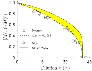
Figure 1: Ground state staggered magnetization, $[M(x)]$, as a function of concentration, $x$, of Zn and Mg in La₂Cu_1-x(Mg/Zn)_xO₄, normalized to the value for zero dilution, $M(0)$  Vajk et al. (2002). The solid line shows the results from quantum Monte Carlo Sandvik (2002) for the site-diluted SLHAF. The figure is reproduced from Ref. [Vajk et al., 2002].

I.4 Ring exchange interactions

One class of candidate perturbations that may be giving the missing physics of diluted La₂CuO₄ are ring, or cyclic, exchange interactions involving multiple interactions around closed plaquettes of the square lattice. Such interactions have received intensive attention recently Notbohm et al. (2007); Gößling et al. (2003); Roger (2005) and have been shown to play an important role in the quantitative description of undiluted La₂CuO₄ Coldea et al. (2001); Toader et al. (2005); Raymond et al. (2006); Toader et al. (2006). Taking as a starting point the one-band half-filled Hubbard model MacDonald et al. (1988); Chernyshev et al. (2004); Delannoy et al. (2005), the lowest order ring exchange interaction takes its origin in virtual electronic hopping process, fourth order in $t/U$, taking electrons coherently around a closed square plaquette. Here $t$ is the nearest neighbor hopping constant and $U$ is the on-site Coulomb energy. Taking it as plausible Toader et al. (2005); Raymond et al. (2006); Toader et al. (2006) that ring exchange is indeed present and a leading perturbation beyond the Heisenberg model description of La₂CuO₄, it is natural to ask what its effect is on the Néel order parameter upon substituting Cu by a concentration $x$ of non-magnetic ions (see Fig. 1). This question, which to the best of our knowledge has so far not been investigated, is the one that we explore in this paper.

To tackle this question, one must return to a problem of correlated electrons. The reason is that the spin-only Hamiltonian with ring exchange derives from a set of electronic hops. As we show below, the elimination of an intermediate site in an electron hopping pathway, affects the resulting effective spin Hamiltonian in a nontrivial manner. Specifically, we consider the problem of a site-diluted half-filled one-band Hubbard model away from the Heisenberg $t/U\rightarrow 0$ limit. Since here ring exchange originates solely from correlated nearest neighbor electronic hops, they cannot move the percolation threshold to a larger value than the nearest neighbor threshold $x_{p}$. From this constraint alone, ring exchange is an admissible candidate for a perturbation to the diluted $S=1/2$ SLHAF, as it preserves the same geometric percolation threshold $x_{p}$ as the nearest neighbor Heisenberg model.

The presence of the ring exchange and second and third nearest neighbor bilinear exchange terms in the Hamiltonian, generated by hopping processes to fourth order in $t/U$, leads to a sign problem for currently available QMC methods using the standard $S^{z}$ basis representation of the Hamiltonian Melko and Kaul (2008). A direct attack on the site-diluted ring exchange Hamiltonian via QMC, such as done for the site-diluted Heisenberg model Sandvik (2002) is therefore not possible at this time. As a first step in investigating the role played by ring exchange in the site-diluted Hubbard model, we carry out a finite-lattice spin wave calculation to order $1/S$ on an extended effective spin Hamiltonian generated from up to four hop electronic pathways. To proceed, we use a real space linear spin wave method adapted to finite-size diluted lattices, first developed by Walker and Walsteadt Walker and Waldstedt (1980) in the context of spin glasses and similar to that used for the site-diluted nearest neighbor Heisenberg antiferromagnet on the square Mucciolo et al. (2004) and honeycomb lattices Castro et al. (2006). We investigate the role of ring exchange on the dependence of the ground state staggered magnetization, $[M(x)]$, as a function of $x$. In Ref. [Mucciolo et al., 2004], it was found that there is a systematic difference between the value of this quantity, calculated via the spin wave method and the essentially exact QMC Sandvik (2002). From this, it is clear that a similar systematic difference should also exist between our data calculated using a $1/S$ expansion, and what would be the not yet available numerically exact value for $[M(x)]$, as a function of dilution, for the extended Hamiltonian. Hence, although the main motivation for this project comes from the experiment on La₂Cu_1-x(Mg/Zn)_xO₄  Vajk et al. (2002), some care has to be taken in attempting to make a direct comparison with experimental results. Rather, our results for the extended Hamiltonian and electronic hopping, can be quantitatively benchmarked by a comparison with those for the site-diluted Heisenberg model, using the same real space expansion technique. From a broader perspective, our work provides a first glimpse at the role of charge correlation effects in the problem of diamagnetic site dilution in the one-band Hubbard model.

I.5 Charge fluctuations

The generation of ring and further neighbor exchange interactions is not the only effect of extending the analysis of the one-band Hubbard model beyond the Heisenberg limit using a perturbation expansion in $t/U$. We have previously shown that extending the expansion to order $(t/U)^{4}$ generates quantum charge fluctuations Delannoy et al. (2005) that are independent of the transverse spin fluctuations of localized $S=1/2$ moments. These fluctuations appear in the perturbation expansion on the square lattice because, to this order, the ground state wave function contains an admixing with excited states corresponding to doubly occupied sites. As doubly occupied sites carry no moment, the expectation value for the magnetic moment of the Hubbard model is reduced below that expected from the effective spin-only Hamiltonian describing transverse spin fluctuations. We show here that these charge fluctuations are a key element in the ultimate success of comparisons between the one-band Hubbard model and experiments on both undiluted and site-diluted La₂CuO₄. Just as for ring exchange effects, we find that the effects of charge fluctuations disappear as the site percolation threshold is approached, as four hop electronic processes are interrupted by the dilution well before this limit is reached.

The rest of the paper is organized as follows: before launching into the calculations, we discuss in Sections IIA and IIB some of the caveats that arise when considering a low energy effective spin-only Hamiltonian derived from a site-diluted Hubbard model. In particular, the exchange interactions become explicitly disorder dependent (Section IIA). Furthermore, by going beyond the Heisenberg limit, the operator for the Néel order parameter has to be corrected to take into account the charge mobility of the electrons in the Hubbard model Delannoy et al. (2005). The results presented below show that this correction is crucially important to obtain the correct $1/S$ behavior of the model. The consequent reduction in the amplitude of the staggered magnetization in the presence of local disorder is discussed in Section IIB. We then discuss in Section IIC the stability of the classical Néel ground state for finite disorder, when ring exchange is present. Section IID describes the spin wave method that we use. Section III gives an overview of the algorithmic procedure used to diagonalize the quadratic form of the disordered finite-lattice spin Hamiltonian. The numerical results are presented in Section IV, followed in Section V by a discussion of the results and a perspective for future work. An appendix discusses the question of statistical uncertainties in the data presented in Section IV.

II Spin Hamiltonian and Real Space Linear Spin Wave Calculation

II.1 Spin Hamiltonian

We begin with the Hubbard Hamiltonian, $H_{\rm H}$:

$$H_{\rm H} = T+V$$ (1)

$$= -t\sum^{\prime}_{i,j;\sigma}\epsilon_{i}\epsilon_{j}c^{\dagger}_{i,\sigma}c^{\phantom{\dagger}}_{j,\sigma}\,+\,U\sum^{\prime}_{i}\epsilon_{i}n_{i,\uparrow}n_{i,\downarrow}.$$ (2)

The first term is the kinetic energy term that destroys an electron of spin $\sigma$ at site $j$ and creates one on the nearest neighbor site $i$. The second term is the on-site Coulomb energy $U$ for two electrons with opposite spins to be on the same site $i$ and where $n_{i,\sigma}=c^{\dagger}_{i,\sigma}c_{i,\sigma}$ is the occupation operator at site $i$. A site $i$ substituted by a non-magnetic cation has $\epsilon_{i}=0$, otherwise $\epsilon_{i}=1$. In the following we use the notation $\sum^{\prime}$ to represent a summation over the $L^{2}$ sites of the square lattice and $\sum$ for a sum over the $N=\sum^{\prime}_{i}(1-\epsilon_{i})$ undiluted sites. The number of magnetic sites and hence of mobile electrons, $N$, at half filling, is thus configuration dependent. The average concentration of vacancies is $1-[\epsilon_{i}]_{\rm disorder}=x$. Similarly, $\sum^{\prime}_{j}$ represents a sum over neighboring sites and $\sum_{j}$ a sum over neighboring occupied magnetic sites. Below, a summation index with angular brackets; $\langle\dots\rangle$ in $\sum_{\langle\ldots\rangle}$ denotes an ordered sum, taking into account only unique pathways.

The derivation of a spin Hamiltonian from a one-band Hubbard model can be performed through many different methods, leading to apparently different effective spin Hamiltonians. It is only recently that it has been shown Chernyshev et al. (2004) that all these Hamiltonians are equivalent, as they are related to each other through a unitary transformation. We have recently applied the canonical transformation method, which uses the ratio $t/U$ as a small parameter in a perturbation expansion, to study the magnetic excitations and the staggered magnetization in the Hubbard model Delannoy et al. (2005, 2008). The method, introduced by Harris et al. Harris and Lange (1967) and developed further by MacDonald et al. MacDonald et al. (1988, 1990, 1991), relies on the separation of the kinetic part $T$ of the Hubbard Hamiltonian into three terms that respectively increase by one ($T_{1}$), keep constant($T_{0}$) or decrease by one ($T_{-1}$) the number of doubly occupied sites. Specifically, one writes:

$$T\,=\,-t\sum^{\prime}_{i,j;\sigma}\epsilon_{i}\epsilon_{j}c^{\dagger}_{i,\sigma}c^{\phantom{\dagger}}_{j,\sigma}\,=\,T_{1}\,+\,T_{0}\,+\,T_{-1}$$ (3)

$$T_{1} = -t\sum^{\prime}_{i,j;\epsilon_{i}\epsilon_{j}\sigma}n_{i,\bar{\sigma}}\epsilon_{i}\epsilon_{j}c^{\dagger}_{i,\sigma}c^{\phantom{\dagger}}_{j,\sigma}h_{j,\bar{\sigma}}$$ (4)

$$T_{0} = -t\sum^{\prime}_{i,j;\sigma}\Big{(}\epsilon_{i}\epsilon_{j}h_{i,\bar{\sigma}}c^{\dagger}_{i,\sigma}c^{\phantom{\dagger}}_{j,\sigma}h_{j,\bar{\sigma}}$$ (5)

$$\qquad+\,n_{i,\bar{\sigma}}c^{\dagger}_{i,\sigma}c^{\phantom{\dagger}}_{j,\sigma}n_{j,\bar{\sigma}}\Big{)}$$

$$T_{-1} = -t\sum^{\prime}_{i,j;\sigma}\epsilon_{i}\epsilon_{j}h_{i,\bar{\sigma}}c^{\dagger}_{i,\sigma}c^{\phantom{\dagger}}_{j,\sigma}n_{j,\bar{\sigma}}$$ (6)

where $\bar{\sigma}$ stands for up if ${\sigma}$ is down and for down if $\sigma$ is up and where $h_{i,\overline{\sigma}}=1-n_{i,\overline{\sigma}}$. This separation comes from multiplying the kinetic term $T$ on the right by $n_{i,\bar{\sigma}}+h_{i,\bar{\sigma}}\,=\,1$ and multiplying on the left by $n_{j,\bar{\sigma}}+h_{j,\bar{\sigma}}\,=\,1$.

Applying a unitary transformation ${\rm e}^{i{\cal S}}$ to $H_{\rm H}$ leads to a spin-only Hamiltonian through the relation:

$$H_{\rm s}\,=\,{\rm e}^{i{\cal S}}H_{\rm H}{\rm e}^{-i{\cal S}}\,=\,H_{\rm H}+{\mathchoice{\dfrac{[i{\cal S},H_{\rm H}]}{1!}}{\dfrac{[i{\cal S},H_{\rm H}]}{1!}}{\frac{[i{\cal S},H_{\rm H}]}{1!}}{\frac{[i{\cal S},H_{\rm H}]}{1!}}}+{\mathchoice{\dfrac{[i{\cal S},[i{\cal S},H_{\rm H}]]}{2!}}{\dfrac{[i{\cal S},[i{\cal S},H_{\rm H}]]}{2!}}{\frac{[i{\cal S},[i{\cal S},H_{\rm H}]]}{2!}}{\frac{[i{\cal S},[i{\cal S},H_{\rm H}]]}{2!}}}+\cdots,$$ (7)

We do not reproduce the derivation here, rather we refer the reader to Refs. [MacDonald et al., 1988; Delannoy et al., 2005, 2008] for details of the form of $\cal S$ and $H_{\rm H}$ order by order in the development. Up to third order in the $t/U$ expansion, we finally find for the effective spin Hamiltonian:

$$H_{\rm s}^{(4)} = \sum_{\langle i,j\rangle}J_{1}\left(\bm{S}_{i}\cdot\bm{S}_{j}\right)$$

$$+ \sum_{\langle\langle i,k\rangle\rangle}J_{2}\left(\bm{S}_{i}\cdot\bm{S}_{k}\right)$$

$$+ \sum_{\langle\langle\langle i,m\rangle\rangle\rangle}J_{3}\left(\bm{S}_{i}\cdot\bm{S}_{m}\right)$$

$$+ \sum_{\langle i,j,k,l\rangle}J_{c}\left\{(\bm{S}_{i}\,\cdot\,\bm{S}_{j})\,(\bm{S}_{k}\,\cdot\,\bm{S}_{l})\right.$$

$$\left.+(\bm{S}_{i}\,\cdot\,\bm{S}_{l})\,(\bm{S}_{k}\,\cdot\,\bm{S}_{j})\,-\,(\bm{S}_{i}\,\cdot\,\bm{S}_{k})\,(\bm{S}_{j}\,\cdot\,\bm{S}_{l})\right\},$$

where the site labels refer to the configuration shown in Fig. 2

Figure 2: Labels for the different sites involved in the effective spin interactions and arising from a $t-U$ Hubbard model up to order $t(t/U)^{3}$. $\langle i,j\rangle$, $\langle\langle i,k\rangle\rangle$, $\langle\langle\langle i,m\rangle\rangle\rangle$ are nearest, second nearest and third nearest neighbors, respectively. $\langle i,j,k,l\rangle$ denotes the sites that belong to an elementary square plaquette.

The different coupling constants $(J_{1},J_{2},J_{3},J_{c})$ arise as a result of the integration over all electronic paths allowed in the site-diluted Hubbard model. As a result, they depend on the local site occupancy along the exchange path. We find:

$$J_{1}=4\left[{\mathchoice{\dfrac{t^{2}}{U}}{\dfrac{t^{2}}{U}}{\frac{t^{2}}{U}}{\frac{t^{2}}{U}}}\epsilon_{i}\epsilon_{j}\,-\,{\mathchoice{\dfrac{t^{4}}{U^{3}}}{\dfrac{t^{4}}{U^{3}}}{\frac{t^{4}}{U^{3}}}{\frac{t^{4}}{U^{3}}}}\left(4\epsilon_{i}\epsilon_{j}+{\cal N}_{ij}\right)\right],$$ (9)

$$J_{2}=4\left[{\mathchoice{\dfrac{t^{4}}{U^{3}}}{\dfrac{t^{4}}{U^{3}}}{\frac{t^{4}}{U^{3}}}{\frac{t^{4}}{U^{3}}}}\left(\epsilon_{i}\epsilon_{j}\epsilon_{k}+\epsilon_{i}\epsilon_{l}\epsilon_{k}-{\cal N}_{ik}\right)\right],$$ (10)

$$J_{3}=4\left[{\mathchoice{\dfrac{t^{4}}{U^{3}}}{\dfrac{t^{4}}{U^{3}}}{\frac{t^{4}}{U^{3}}}{\frac{t^{4}}{U^{3}}}}\epsilon_{i}\epsilon_{j}\epsilon_{m}\right],$$ (11)

$$J_{c}=80\left[{\mathchoice{\dfrac{t^{4}}{U^{3}}}{\dfrac{t^{4}}{U^{3}}}{\frac{t^{4}}{U^{3}}}{\frac{t^{4}}{U^{3}}}}\epsilon_{i}\epsilon_{j}\epsilon_{k}\epsilon_{l}\right],$$ (12)

where ${\cal N}_{\mu\nu}$ is a plaquette index for bond $\mu\nu$ and is equal to the number of plaquettes to which both sites $\mu$ and $\nu$ belong. When there is no dilution, ${\cal N}_{\mu\nu}=2$ for all nearest neighbor $\langle i,j\rangle$ bonds and $1$ for second neighbor bonds $\langle\langle i,j\rangle\rangle$ across the diagonal of a plaquette. When one of the four bonds defining a plaquette is missing, the ${\cal N}_{\mu\nu}$ for the three nearest neighbor bonds along the remaining edges of the plaquette are reduced from two to one. ${\cal N}_{\mu\nu}$ for the next nearest neighbor bond across the diagonal of the plaquette is reduced from one to zero. For example, consider Fig. 2 where only the site $j$ has been eliminated by dilution. The expression for the coupling constants becomes:

$$\begin{array}[]{lcl}J_{1}(i,l)&=&4{\mathchoice{\dfrac{t^{2}}{U}}{\dfrac{t^{2}}{U}}{\frac{t^{2}}{U}}{\frac{t^{2}}{U}}}-20{\mathchoice{\dfrac{t^{4}}{U^{3}}}{\dfrac{t^{4}}{U^{3}}}{\frac{t^{4}}{U^{3}}}{\frac{t^{4}}{U^{3}}}}\\ \\ J_{2}(i,k)&=&4{\mathchoice{\dfrac{t^{4}}{U^{3}}}{\dfrac{t^{4}}{U^{3}}}{\frac{t^{4}}{U^{3}}}{\frac{t^{4}}{U^{3}}}}\\ \\ J_{3}(i,m)&=&0\,\,\,\,\,\,\,\,\,\,\,\,J_{c}(i,j,k,l)\,=\,0,\end{array}$$ (13)

which should be compared with $J_{1}=4t^{2}/U-24t^{4}/U^{3}$, $J_{2}=J_{3}=4t^{4}/U^{3}$ and $J_{c}=80t^{4}/U^{3}$ for the undiluted lattice. The most important point here is that since the antiferromagnetic and frustrating $J_{2}$ and $J_{3}$ exist solely via electronic hopping processes connecting nearest neighbor sites, these interactions are progressively eliminated as intermediate sites are diluted. That is, if both sites $j$ and $l$ are missing then $J_{2}(i,k)=0$. Hence, one can see that site dilution strongly affects the coupling constants as further neighbor exchange depends on the existence of a nearest neighbor pathway between the sites. This would not be the case if the original Hubbard model included direct second or third nearest neighbor hopping parameters, $t^{\prime}$ and $t^{\prime\prime}$, respectively Delannoy et al. (2008). We will return to this issue in the Conclusion section. However, in this paper we limit ourselves to nearest neighbor hopping only.

II.2 Néel order parameter

Our objective is to calculate the ground state Néel order parameter for the original Hubbard model as a function of site dilution, using a spin-only description. To do this, the staggered (spin density wave) magnetization operator,

$$\hat{M}_{\rm H}\,=\,{\mathchoice{\dfrac{1}{N}}{\dfrac{1}{N}}{\frac{1}{N}}{\frac{1}{N}}}\sum_{i}(-1)^{i}(n_{i}^{\uparrow}-n_{i}^{\downarrow}),$$ (14)

defined for the Hubbard model, must be canonically transformed before it can be exploited in a spin-only description. Here, $\hat{M}_{\rm H}$, $\hat{M}_{\rm s}$ and ${\hat{\widetilde{M}}_{\rm s}}$ refer to operators while $M_{\rm s}$ and ${{\widetilde{M}}_{\rm s}}$ refer to their expectation values. That is, within the effective theory $M_{\rm H}$ becomes $\hat{M}_{\rm s}=e^{i{\cal S}}\hat{M}_{\rm H}e^{-i{\cal S}}$ and the expectation value in the ground state is defined

$$M_{\rm s}\,=\,\frac{{}_{\rm H}\langle 0|\hat{M}_{\rm H}|0\rangle_{\rm H}}{{}_{\rm H}\langle 0|0\rangle_{\rm H}}\,=\,\frac{{}_{\rm s}\langle 0|{\hat{M}_{\rm s}}|0\rangle_{\rm s}}{{}_{\rm s}\langle 0|0\rangle_{\rm s}}\;\;\;.$$ (15)

Here $|0\rangle_{\rm H}$ and $|0\rangle_{\rm s}=e^{i{\cal S}}|0\rangle_{\rm H}$ are the ground state wave vectors in the original Hubbard and spin-only models. We have recently shown Delannoy et al. (2005) that this is more than just an academic point. Rather, it has important consequences for the ground state magnetization as one moves into the intermediate coupling regime and, as we will show below, plays a significant quantitative role in the present site-diluted Hubbard model. As we apply the canonical transformation on $\hat{M}_{\rm H}$ Delannoy et al. (2005, 2008) we find for $\hat{M}_{\rm s}$:

$$\hat{M}_{\rm s}\,=\,\hat{M}_{\rm H}\,+\,{\mathchoice{\dfrac{1}{U}}{\dfrac{1}{U}}{\frac{1}{U}}{\frac{1}{U}}}\left(\tilde{T}_{1}-\tilde{T}_{-1}\right)\,+\,{\mathchoice{\dfrac{1}{2U^{2}}}{\dfrac{1}{2U^{2}}}{\frac{1}{2U^{2}}}{\frac{1}{2U^{2}}}}\left(\tilde{T}_{-1}T_{1}-T_{-1}\tilde{T}_{1}\right),$$ (16)

where

$${\mathchoice{\dfrac{1}{N}}{\dfrac{1}{N}}{\frac{1}{N}}{\frac{1}{N}}}\tilde{T}_{1} \equiv [T_{1},\hat{M}_{H}],$$ (17)

$${\mathchoice{\dfrac{1}{N}}{\dfrac{1}{N}}{\frac{1}{N}}{\frac{1}{N}}}\tilde{T}_{-1} \equiv [T_{-1},\hat{M}_{H}],$$ (18)

$${\mathchoice{\dfrac{1}{N}}{\dfrac{1}{N}}{\frac{1}{N}}{\frac{1}{N}}}\tilde{T}_{0} \equiv [T_{0},\hat{M}_{H}].$$ (19)

After some algebra, we can write this expression in terms of $S=1/2$ spin operatorsDelannoy et al. (2005) as:

$$\hat{M}_{\rm s} = {\mathchoice{\dfrac{1}{N}}{\dfrac{1}{N}}{\frac{1}{N}}{\frac{1}{N}}}\sum^{\prime}_{i}\epsilon_{i}S_{i}^{z}(-1)^{i}$$ (20)

$$- {\mathchoice{\dfrac{2t^{2}}{NU^{2}}}{\dfrac{2t^{2}}{NU^{2}}}{\frac{2t^{2}}{NU^{2}}}{\frac{2t^{2}}{NU^{2}}}}\sum^{\prime}_{\langle i,j\rangle}\epsilon_{i}\epsilon_{j}\left\{S_{i}^{z}\,-\,S_{j}^{z}\right\}(-1)^{i}.$$

Recalling the standard definition for the staggered magnetization operator in a spin model,

$${\hat{\widetilde{M}}_{\rm s}}={\mathchoice{\dfrac{1}{N}}{\dfrac{1}{N}}{\frac{1}{N}}{\frac{1}{N}}}\sum_{i}^{\prime}\epsilon_{i}S_{i}^{z}(-1)^{i},$$ (21)

we arrive at the principal result of Ref. [Delannoy et al., 2005] that

$$M_{\rm s} = \frac{{}_{\rm s}\langle 0|{\hat{M}_{\rm s}}|0\rangle_{\rm s}}{{}_{\rm s}\langle 0|0\rangle_{\rm s}}$$

$${\widetilde{M}_{\rm s}} = \,\frac{{}_{\rm s}\langle 0|{\hat{\widetilde{M}}_{\rm s}}|0\rangle_{\rm s}}{{}_{\rm s}\langle 0|0\rangle_{\rm s}}$$

$${\rm and}$$

$$M_{\rm s} \neq {\widetilde{M}_{\rm s}}.$$ (22)

The difference is due to the appearance of new quantum fluctuations arising from the charge delocalization over closed virtual loops of electronic hops, which is the origin of the second term in Eq. (20). These spin independent fluctuations, which appear to order $t^{2}/U^{2}$ in the magnetization operator, are generated when the canonical transformation is applied on the Hamiltonian to order $t^{4}/U^{3}$ and are therefore not present in the $(t/U\rightarrow 0)$ Heisenberg limit. We recently investigated the effects of these terms in the undiluted case Delannoy et al. (2005, 2008). Here, the disorder is manifest through the dilution variables $\epsilon_{i}$ and, in this paper, we are interested in how the spin renormalization factor modifies the ground state magnetization upon site dilution. However, before doing so, we first return to a discussion of the ground state of the spin-only Hamiltonian $H_{\rm s}^{(4)}$.

Henceforth, for the sake of compactness, we shall omit the subscript “s” in $M_{\rm s}$ and ${\widetilde{M}}_{\rm s}$, understanding that all results presented below were obtained from calculations performed on a spin-only description of the low-energy sector of the half-filled Hubbard model.

II.3 Classical ground state

II.3.1 $J_{1}$ interactions only

The real space spin wave method that we use to deal with dilution requires, as the starting point, the knowledge of the classical ground state spin configuration. With nearest neighbor interactions only, the classical ground state configuration is, in the absence of dilution, the Néel staggered spin configuration. This long range ordered state results from the local minimization of the exchange interactions. Since we work with a concentration of defects, or dilution, $x$, smaller than the percolation threshold $x_{p}$, there exists a percolating cluster of magnetic sites with an exchange path connecting every pair of spins on the cluster. As a result, the classical ground state configuration for the percolating cluster is a connected Néel configuration, where every spin keeps the orientation it would have had without dilution (see Fig. 3).

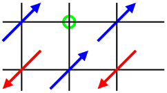
Figure 3: Diluted Néel configuration. The circle labels a missing (diluted) site.

II.3.2 Full Hamiltonian

In the case of the effective spin-only Hamiltonian, expressed in Eq. (II.1), the situation becomes more complicated. If the $J_{2}$, $J_{3}$ or $J_{c}$ interactions get too large, the system undergoes a phase transition to a new classical state that is not collinear.

Non diluted case

As can be read from Eqs. (9,10,12), when there is no dilution, the coupling constants read:

$$\left\{\begin{array}[]{ccl}J_{1}&=&4{\mathchoice{\dfrac{t^{2}}{U}}{\dfrac{t^{2}}{U}}{\frac{t^{2}}{U}}{\frac{t^{2}}{U}}}-24{\mathchoice{\dfrac{t^{4}}{U^{3}}}{\dfrac{t^{4}}{U^{3}}}{\frac{t^{4}}{U^{3}}}{\frac{t^{4}}{U^{3}}}}\\ J_{2}&=&J_{3}=\,4{\mathchoice{\dfrac{t^{4}}{U^{3}}}{\dfrac{t^{4}}{U^{3}}}{\frac{t^{4}}{U^{3}}}{\frac{t^{4}}{U^{3}}}}\\ J_{c}&=&80{\mathchoice{\dfrac{t^{4}}{U^{3}}}{\dfrac{t^{4}}{U^{3}}}{\frac{t^{4}}{U^{3}}}{\frac{t^{4}}{U^{3}}}}\\ \end{array}\right.$$ (23)

For $t/U\,=\,1/8$, a value similar to that reported for La₂CuO₄ and that we henceforth take in the present work Coldea et al. (2001); Delannoy et al. (2008), the ratios between the different coupling constants are:

$$\left\{\begin{array}[]{ccl}{\mathchoice{\dfrac{J_{2}}{J_{1}}}{\dfrac{J_{2}}{J_{1}}}{\frac{J_{2}}{J_{1}}}{\frac{J_{2}}{J_{1}}}}&\simeq&0.0172,\\ {\mathchoice{\dfrac{J_{3}}{J_{1}}}{\dfrac{J_{3}}{J_{1}}}{\frac{J_{3}}{J_{1}}}{\frac{J_{3}}{J_{1}}}}&\simeq&0.0172,\\ {\mathchoice{\dfrac{J_{c}}{J_{1}}}{\dfrac{J_{c}}{J_{1}}}{\frac{J_{c}}{J_{1}}}{\frac{J_{c}}{J_{1}}}}&\simeq&0.0862.\\ \end{array}\right.$$ (24)

For a model with nearest and next nearest couplings only, the $J_{1}/J_{2}$ model, the Néel state is stable for ${J_{2}}/{J_{1}}\leqslant 0.5$  Chandra and Doucot (1988); Dagotto and Moreo (1989); Young (1995). For the $J_{1}/J_{c}$ model, the quantity $\displaystyle\tilde{J_{c}}\,=\,J_{c}\,S^{2}$ is usually introduced, and as long as $\displaystyle\tilde{J_{c}}\,\leqslant\,{J}/{2}$, the Néel state is stable Chubukov et al. (1992). Our parameters are far away from these critical values, and hence the classical ground state, without dilution, is Néel ordered.

Diluted case

One might have expected that the combination of frustration, brought about by $J_{2}$ and $J_{3}$ and site dilution would trigger an instability in favor of a local Villain canting of the spins Villain (1979), leading ultimately to a two dimensional Heisenberg spin glass before $x_{p}$ is reached Gawiec and Grempel (1991).

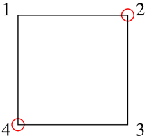
Figure 4: Particular dilution configuration. In this example, sites $2$ and $4$ are removed by dilution.

However, as alluded to in the discussion below Eq. (13), such locally Villain canted states do not occur in the model considered here, where all effective magnetic interactions derive from electronic processes involving nearest neighbor hopping. Hence, as we saw in the previous section, for the configuration of diluted sites shown in Fig. 4 the second neighbor interaction, $J_{13}$, between sites 1 and 3 is destroyed by the dilution of sites 2 and 4. As a consequence, as long as the critical ratios for the $J_{2}/J_{1}$, $J_{3}/J_{1}$ or $J_{c}/J_{1}$ for destroying two sublattice collinear Néel order are not reached, there are no spins coupled by dominantly random frustrating interactions, $J_{2}$, $J_{3}$ or $J_{c}$, as can be verified from studying Eqs. (9,10,12).

We therefore conclude that the classical ground state of $H_{\rm s}^{(4)}$ in Eq. (II.1) for $t/U=1/8$ on the percolation cluster is a Néel configuration for all concentrations below the percolation threshold. From this, one can immediately see the importance of the site percolation threshold in this problem: within the model considered, that is the site-diluted one-band Hubbard model of Eq. 2, the only accessible classical ground state is Néel ordered all the way to the percolation threshold $x_{p}$. Hence, any reduction in the range of stability of the Néel ground state is due uniquely to quantum fluctuations and is not due to (classical) random frustration effects. This conclusion is explicitly verified post factum within the real space spin wave calculation: any instability towards a non-collinear ground state would be detected as a negative eigenvalue of the Hessian matrix leading to complex eigenfrequencies. No such instabilities were detected in more than the ten thousand realizations of disorder considered in this work.

We note, however, that La₂CuO₄ is only approximately described by the one-band Hubbard model with nearest neighbor hopping only. For instance we have recently shown that one can achieve a quantitative improvement to the fitting of the spin wave excitation spectrum measured by Coldea et al. Coldea et al. (2001) by including direct further neighbor hopping constants $t^{\prime}$ and $t^{\prime\prime}$  Delannoy et al. (2008). Such direct hops could change the above results, leading to canted classical ground states Villain (1979); Binder et al. (1979); Parker and Saslow (1988); Saslow and Parker (1988); Vannimenus et al. (1989); Gawiec and Grempel (1991) before the percolation threshold is reached ($x_{c}<x_{p}$).

II.4 Elementary excitations of a diluted spin $1/2$ system

II.4.1 Method

The introduction of site dilution destroys translational invariance, which excludes the use of Fourier space for calculating the spin-wave excitations. Hence, we closely follow the method introduced by Walker and Waldstedt Walker and Waldstedt (1980) to study excitations in Heisenberg spin glasses. Other recent studies of site-diluted $S=1/2$ Heisenberg antiferromagnets have followed a similar approach Mucciolo et al. (2004); Castro et al. (2006). We first summarize this method for the simplest case of nearest neighbor exchange, $J_{1}$ only, with Hamiltonian

$$H=\frac{1}{2}\sum_{\langle i,j\rangle}J_{1}(i,j)\bm{S}_{i}\cdot\bm{S}_{j}.$$ (25)

As we know the classical ground state of the system, we can define for each site $i$, a unit vector ${\bm{n}}_{i}^{0}$ pointing in the direction of the classical spin ${\bm{S}}_{i}$ in this state. Note that in Eqs.(14,20,21) a unique global quantization axis in the lab frame, $\hat{z}$ , was used to define ${\widetilde{M}}_{\rm s}$ and $M_{\rm s}$. Henceforth, we label the spin components in terms of the projection of ${\bm{S}}_{i}$ along the axis of a local right handed frame. We do so to keep with the original notation of Ref. [Walker and Waldstedt, 1980], from which we borrowed the method we use here. Let $\{{\bm{x}}_{i},{\bm{y}}_{i},{\bm{n}}_{i}^{0}\}$ be an orthogonal triad of unit vectors and let ${\bm{p}}_{i}^{+}$ and ${\bm{p}}_{i}^{-}$ be vectors defined by

$$\begin{array}[]{ccl}{{\bm{p}}_{i}^{+}}&=&{\mathchoice{\dfrac{{{\bm{x}}_{i}}+i{{\bm{y}}_{i}}}{\sqrt{2}}}{\dfrac{{{\bm{x}}_{i}}+i{{\bm{y}}_{i}}}{\sqrt{2}}}{\frac{{{\bm{x}}_{i}}+i{{\bm{y}}_{i}}}{\sqrt{2}}}{\frac{{{\bm{x}}_{i}}+i{{\bm{y}}_{i}}}{\sqrt{2}}}},\\ \\ {{\bm{p}}_{i}^{-}}&=&{\mathchoice{\dfrac{{{\bm{x}}_{i}}-i{{\bm{y}}_{i}}}{\sqrt{2}}}{\dfrac{{{\bm{x}}_{i}}-i{{\bm{y}}_{i}}}{\sqrt{2}}}{\frac{{{\bm{x}}_{i}}-i{{\bm{y}}_{i}}}{\sqrt{2}}}{\frac{{{\bm{x}}_{i}}-i{{\bm{y}}_{i}}}{\sqrt{2}}}}.\end{array}$$ (26)

We also introduce spin deviation (boson creation and annihilation operators), $a_{i}$ and $a_{i}^{\dagger}$, defined by

$${\bm{S}}_{i}\cdot{\bm{n}}_{i}^{0} = S-a_{i}^{\dagger}\,a_{i}\;\;\;,$$

$${\bm{S}}_{i}\cdot{\bm{p}}_{i}^{+} = \sqrt{2S}{\left[1-\frac{a_{i}^{\dagger}\,a_{i}}{2S}\right]}^{\frac{1}{2}}a_{i}\;\;\;,$$ (28)

$${\bm{S}}_{i}\cdot{\bm{p}}_{i}^{-} = \sqrt{2S}a_{i}^{\dagger}{\left[1-\frac{a_{i}^{\dagger}\,a_{i}}{2S}\right]}^{\frac{1}{2}},$$

where the spin components are defined with respect to the local basis set, $\{{\bm{x}}_{i},{\bm{y}}_{i},{\bm{n}}_{i}^{0}\}$. With Eq. II.4.1 and the definition of ${\bm{p}}_{i}^{\pm}$, we can rewrite the Hamiltonian Eq. 25 to order $O(S)$ as:

$$\begin{split}H&=\frac{1}{2}S^{2}\sum_{\langle i,j\rangle}J_{ij}{{\bm{n}}_{i}^{0}}\cdot{{\bm{n}}_{j}^{0}}\\ &+\frac{1}{2}S^{3/2}\sum_{\langle i,j\rangle}J_{ij}\Big{[}{{\bm{n}}_{i}^{0}}\cdot{{\bm{p}}_{j}^{+}}a_{j}^{{\dagger}}+{{\bm{n}}_{i}^{0}}\cdot{{\bm{p}}_{j}^{-}}a_{j}\\ &\quad+\;{{\bm{n}}_{j}^{0}}\cdot{{\bm{p}}_{i}^{+}}a_{i}^{{\dagger}}+{{\bm{n}}_{j}^{0}}\cdot{{\bm{p}}_{i}^{-}}a_{i}\Big{]}\\ &+\frac{1}{2}S\sum_{\langle i,j\rangle}J_{ij}\Big{[}({{\bm{p}}_{i}^{+}}a_{i}^{{\dagger}}+{{\bm{p}}_{i}^{-}}a_{i})\cdot({{\bm{p}}_{j}^{+}}a_{j}^{{\dagger}}+{{\bm{p}}_{j}^{-}}a_{j})\\ &\quad-\ {{\bm{n}}_{i}^{0}}\cdot{{\bm{n}}_{j}^{0}}(a_{i}^{{\dagger}}a_{i}+a_{j}^{{\dagger}}a_{j})\Big{]}\;.\end{split}$$ (29)

By making reference to the classical ground state, we introduce $\lambda_{i}$ defined by

$$\sum_{j}J_{ij}\bm{n}_{j}^{0}=\lambda_{i}\bm{n}_{i}^{0}\;\;\;.$$ (30)

Physically, $\lambda_{i}$ corresponds to the local staggered mean-field at site $i$ originating from all the spins ${\bm{S}}_{j}$ to which ${\bm{S}}_{i}$ is coupled. This change of variables makes the second term of the Hamiltonian vanish. We keep only the leading quantum correction to the classical term $\frac{1}{2}S^{2}\sum_{\langle i,j\rangle}{{\bm{n}}_{i}^{0}}\cdot{{\bm{n}}_{j}^{0}}$, $H_{2}$, quadratic in the $\{a_{i}^{\dagger},a^{\phantom{\dagger}}_{i}\}$:

$$\begin{array}[]{ccl}H_{2}&=&\displaystyle S\left[\sum_{i}\lambda_{i}a_{i}^{{\dagger}}\,a_{i}\right.\\ &&\displaystyle\left.\,-\,\frac{1}{2}\sum_{\langle i,j\rangle}J_{ij}({{\bm{p}}_{i}^{+}}a_{i}^{{\dagger}}+{{\bm{p}}_{i}^{-}}a_{i})\cdot({{\bm{p}}_{j}^{+}}a_{j}^{{\dagger}}+{{\bm{p}}_{j}^{-}}a_{j})\right]\end{array}$$ (31)

The quantum-mechanical equations of motion are:

$$-i\frac{da_{i}^{{\dagger}}}{dt}=\left[H_{2},a_{i}^{{\dagger}}\right],$$

(32)

$$-i\frac{da_{i}}{dt}=\left[H_{2},a_{i}\right],$$

which can be written:

$${\mathchoice{\dfrac{da_{i}}{dt}}{\dfrac{da_{i}}{dt}}{\frac{da_{i}}{dt}}{\frac{da_{i}}{dt}}}=-i\left(\sum_{j}Q_{ij}a_{j}^{{\dagger}}\,+\,\sum_{j}P_{ij}a_{j}\right),$$

(33)

$${\mathchoice{\dfrac{da_{i}^{{\dagger}}}{dt}}{\dfrac{da_{i}^{{\dagger}}}{dt}}{\frac{da_{i}^{{\dagger}}}{dt}}{\frac{da_{i}^{{\dagger}}}{dt}}}=i\left(\sum_{j}Q_{ij}^{*}a_{j}\,+\,\sum_{j}P_{ij}^{*}a_{j}^{{\dagger}}\right),$$

where $P_{ij}={\lambda_{i}}\delta_{ij}-{J_{ij}}({{\bm{p}}_{i}}^{+}\cdot{{\bm{p}}_{j}}^{-})$ and $Q_{ij}=-{J_{ij}}({{\bm{p}}_{i}}^{+}\cdot{{\bm{p}}_{j}}^{+})$. We use a vector representation for the operators $a_{i}$ and $a_{i}^{{\dagger}}$; that is $a$ and $a^{{\dagger}}$ are $N$-dimensional vectors whose components are $a_{i}$ and $a_{i}^{{\dagger}}$, respectively. As $N$, the total number of (occupied) magnetic sites, is configuration dependent, so are all vectors and matrices in the following discussion. We write

$${\mathchoice{\dfrac{d}{dt}}{\dfrac{d}{dt}}{\frac{d}{dt}}{\frac{d}{dt}}}\left(\begin{array}[]{c}a\\ a^{{\dagger}}\end{array}\right)\;=\;i\,\,\left(\begin{array}[]{cc}-P&-Q\\ Q^{*}&P^{*}\end{array}\right)\;\left(\begin{array}[]{c}a\\ a^{{\dagger}}\end{array}\right),$$ (34)

where we refer to $P$ and $Q$ as the “interaction matrices” of order $N\times N$. We can also write

$$H_{2}=S\left(a^{{\dagger}}\;a\right)\;{\widetilde{H}}\;\left(\begin{array}[]{c}a\\ a^{{\dagger}}\end{array}\right)$$ (35)

where the Hamiltonian matrix $\widetilde{H}$ is defined in the $2N\times 2N$ phase space to be:

$$\widetilde{H}=\left(\begin{array}[]{cc}-P&-Q\\ Q^{*}&P^{*}\end{array}\right).$$ (36)

In order to diagonalize $\widetilde{H}$, we perform a Bogoliubov transformation that introduces new boson operators $d$ and $d^{{\dagger}}$, as follows:

$$a = g^{*}\,d+f\,d^{{\dagger}}$$

$$a^{{\dagger}} = f^{*}\,d+g\,d^{{\dagger}}$$

$f$ and $g$ are $N\times N$ matrices that must satisfy the boson commutation rules:

$$g^{*}\,f^{T}-f\,g^{{\dagger}} = 0$$

$$g^{*}\,g^{T}-f\,f^{{\dagger}} = 1\;\;\;,$$

where $f^{T}$ is the transpose matrix of $f$. We can also write these relationships in matrix representation:

$$\widetilde{E}\;\widetilde{I}\;\widetilde{E}^{{\dagger}}\;=\;\widetilde{I}$$ (38)

where

$$\widetilde{E}=\left(\begin{array}[]{cc}g^{*}&f\\ f^{*}&g\end{array}\right),\;\;\;\widetilde{I}=\left(\begin{array}[]{cc}-1&0\\ 0&1\end{array}\right),$$ (39)

are of dimension $2N\times 2N$.

The aim of the Bogoliubov transformation is to diagonalize Eq.(34). Consequently we require

$${\mathchoice{\dfrac{d}{dt}}{\dfrac{d}{dt}}{\frac{d}{dt}}{\frac{d}{dt}}}\left(\begin{array}[]{c}d\\ d^{{\dagger}}\end{array}\right)\,\,=\,\,i\left(\begin{array}[]{cc}-\Omega&0\\ 0&\Omega\end{array}\right)\left(\begin{array}[]{c}d\\ d^{{\dagger}}\end{array}\right)$$ (40)

where $\Omega$ is a diagonal matrix of eigenfrequencies. Using (34) and (39) one obtains:

$${\mathchoice{\dfrac{d}{dt}}{\dfrac{d}{dt}}{\frac{d}{dt}}{\frac{d}{dt}}}\left(\begin{array}[]{cc}g^{*}&f\\ f^{*}&g\end{array}\right)\left(\begin{array}[]{c}d\\ d^{{\dagger}}\end{array}\right)$$ (45)

$$\qquad\qquad=i\left(\begin{array}[]{cc}g^{*}&f\\ f^{*}&g\end{array}\right)\left(\begin{array}[]{cc}-\Omega&0\\ 0&\Omega\end{array}\right)\left(\begin{array}[]{c}d\\ d^{{\dagger}}\end{array}\right)$$ (52)

$$\qquad\qquad=i\left(\begin{array}[]{cc}-P&-Q\\ Q^{*}&P^{*}\end{array}\right)\left(\begin{array}[]{cc}g^{*}&f\\ f^{*}&g\end{array}\right)\left(\begin{array}[]{c}d\\ d^{{\dagger}}\end{array}\right).$$ (59)

Hence, the equation we ultimately have to solve is:

$$\widetilde{E}D=\widetilde{H}\widetilde{E},$$ (60)

where we have defined the complete matrix of eigenvalues:

$$D=\left(\begin{array}[]{cc}-\Omega&0\\ 0&\Omega\end{array}\right)\;\;\;.$$ (61)

With this method, we can calculate the zero point quantum spin fluctuations to order $1/S$, and hence the expectation value for the spin on occupied site $i$:

$$\langle S_{i}^{z}\rangle\,=\,S-{\langle a_{i}^{{\dagger}}a_{i}\rangle}=S-\sum_{\nu}|f_{i\nu}|^{2}.$$ (62)

With the expectation value $\langle S_{i}^{z}\rangle$ now defined in terms of $|f_{i\nu}|^{2}$, one can calculate the staggered magnetization, defined in either Eq. (20) for the finite $t/U$ Hubbard model or Eq. (21) for the $t/U\rightarrow 0$ Heisenberg model. Formally speaking, in a thermodynamically large system, spins that reside on finite-size clusters and which are connected to the percolating cluster do not participate to the symmetry breaking nor do they contribute to the average bulk staggered magnetization. Hence, to capture that physics in the present problem, and to proceed numerically, numerically, we first identify for a given realization of disorder, a percolating cluster of sites connected via nearest neighbor hopping. For each spin on the percolating cluster, $\langle S_{i}^{z}\rangle$ is determined from Eq. (62), summed over, and normalized by $N$, the total number of sites for that realization of disorder (percolating and not), to give $M_{\rm s}$ in Eq. (20) (henceforth denoted $M$). One then repeats the calculation for many dilution configurations for a given $x$, performing a disorder average and obtaining both the averaged staggered magnetization on the percolating cluster, $[M(x)]_{\rm perc}$, or the bulk staggered magnetization, $[M(x)]$, averaged over all magnetic sites in the sample. We stress that, while the staggered magnetization on the percolating cluster, $[M(x)]_{\rm perc}$ is the most relevant quantity for the numerical study, it is the average staggered magnetization over all Cu magnetic sites in the system, percolating and not, $[M(x)]$, which is accessible to experiment, and which is displayed in Fig. 1.

In the presence of interactions beyond $J_{1}(i,j)$, the only change in the details of the above method occur in the matrix elements of $P$ and $Q$. The form of these matrices, taking into account the second ($J_{2}$), third ($J_{3}$) and ring ($J_{c}$) exchange interactions is discussed next.

II.4.2 Calculation of the $P$ and $Q$ matrices

$J_{1}$: first NN

In this case the quadratic Hamiltonian reads:

$$H_{2}(J_{1})=S\sum_{\langle i,j\rangle}J_{1}(i,j)\left(a_{i}^{{\dagger}}a_{i}+a_{j}^{{\dagger}}a_{j}-a_{i}a_{j}-a_{i}^{{\dagger}}a_{j}^{{\dagger}}\right).$$ (63)

The $P$ and $Q$ interaction matrices then have the following form:

$$P\,=\,\left(\begin{array}[]{cccc}\lambda_{1}\\ &\ddots\\ &&\ddots\\ &&&\lambda_{L^{2}}\end{array}\right)$$,

(64)

where $\lambda_{i}$ is defined in Eq. (30), and $Q$ is a symmetric matrix $Q_{ij}\,=\,-J_{1}(i,j)$.

$J_{2}$: Second NN

We have:

$$H_{2}(J_{2})=-S\sum_{\langle\langle i,j\rangle\rangle}J_{2}(i,j)\left(a_{i}^{{\dagger}}a_{i}+a_{j}^{{\dagger}}a_{j}-a_{i}^{{\dagger}}a_{j}-a_{j}^{{\dagger}}a_{i}\right),$$ (65)

which leads to the following additions to the $P$ and $Q$ matrices:

$$P^{(2)} =\left(\begin{array}[]{cccc}\lambda_{1}^{(2)}\\ &\ddots&-J_{2}\\ &-J_{2}&\ddots\\ &&&\lambda_{L^{2}}^{(2)}\end{array}\right),$$ (70)

$$Q^{(2)} =\left(\begin{array}[]{cccc}0&&&0\\ \vdots&\ddots&&\vdots\\ \vdots&&\ddots&\vdots\\ 0&&&0\end{array}\right)$$ (75)

$\lambda_{i}^{(2)}$ is defined in a similar way to $\lambda_{i}$:

$$\sum_{\langle\langle j\rangle\rangle}J_{2}(i,j)\bm{n}_{j}^{0}=\lambda_{i}^{(2)}\bm{n}_{i}^{0},$$ (76)

where $\langle\langle j\rangle\rangle$ indicates a sum over the second neighbors of site $i$.

$J_{3}$: Third NN

$$H_{2}(J_{3})=-S\!\!\sum_{\langle\langle\langle i,j\rangle\rangle\rangle}\!\!J_{3}(i,j)\left(a_{i}^{{\dagger}}a_{i}+a_{j}^{{\dagger}}a_{j}-a_{i}^{{\dagger}}a_{j}-a_{j}^{{\dagger}}a_{i}\right),$$ (77)

hence the expression for the $P$ and $Q$ matrices are modified by:

$$P^{(3)} =\left(\begin{array}[]{cccc}\lambda_{1}^{(3)}\\ &\ddots&-J_{3}\\ &-J_{3}&\ddots\\ &&&\lambda_{L^{2}}^{(3)}\end{array}\right),$$ (82)

$$Q^{(3)} =\left(\begin{array}[]{cccc}0&&&0\\ \vdots&\ddots&&\vdots\\ \vdots&&\ddots&\vdots\\ 0&&&0\end{array}\right)$$ (87)

with $\lambda_{i}^{(3)}$ defined by:

$$\sum_{\langle\langle\langle j\rangle\rangle\rangle}J_{3}(i,j)\bm{n}_{j}^{0}=\lambda_{i}^{(3)}\bm{n}_{i}^{0},$$ (88)

where $\langle\langle\langle j\rangle\rangle\rangle$ indicates the third neighbors of site $i$.

$J_{c}$: Ring exchange interaction

To first order in $1/S$, the four spin terms appearing in the Hamiltonian are decoupled into bilinear products of $a_{i}^{\dagger}a_{j}$. That is, to order $1/S$, the net effect of the ring exchange is to simply renormalize the $J_{1}$ and $J_{2}$ interactions Coldea et al. (2001); Toader et al. (2005); Delannoy et al. (2005). The contribution of the ring exchange terms to the quadratic Hamiltonian is thus:

$$\begin{split}H_{2}(J_{c})&=\displaystyle-S^{3}\sum_{\langle i,j,k,l\rangle}J_{c}(i,j,k,l)\left[\left(a_{i}^{{\dagger}}a_{i}+a_{j}^{{\dagger}}a_{j}+a_{k}^{{\dagger}}a_{k}+a_{l}^{{\dagger}}a_{l}\right)+\left(a_{i}^{{\dagger}}a_{k}+a_{k}^{{\dagger}}a_{i}+a_{j}^{{\dagger}}a_{l}+a_{l}^{{\dagger}}a_{j}\right)\right.\\ &\left.\qquad\qquad-\ \left(a_{i}^{{\dagger}}a_{j}+a_{j}^{{\dagger}}a_{i}+a_{i}^{{\dagger}}a_{l}+a_{l}^{{\dagger}}a_{i}+a_{j}^{{\dagger}}a_{k}+a_{k}^{{\dagger}}a_{j}+a_{k}^{{\dagger}}a_{l}+a_{l}^{{\dagger}}a_{k}\right)\right],\end{split}$$

where $J_{c}(i,j,k,l)=\epsilon_{i}\epsilon_{j}\epsilon_{k}\epsilon_{l}J_{c}$. The elements of the Bogoliubov transformation matrices $g$ and $f$ are thus modified by the configuration dependent renormalization of the first and second neighbor exchanges. In zero dilution, $J_{1}$ and $J_{2}$ are renormalized to Coldea et al. (2001); Toader et al. (2005); Delannoy et al. (2005):

$$\left\{\begin{array}[]{cclcl}J_{1}^{\rm eff}&=&J_{1}-2S^{2}J_{c}&=&J_{1}-{\mathchoice{\dfrac{J_{c}}{2}}{\dfrac{J_{c}}{2}}{\frac{J_{c}}{2}}{\frac{J_{c}}{2}}}\\ \\ J_{2}^{\rm eff}&=&J_{2}-S^{2}J_{c}&=&J_{2}-{\mathchoice{\dfrac{J_{c}}{4}}{\dfrac{J_{c}}{4}}{\frac{J_{c}}{4}}{\frac{J_{c}}{4}}};\end{array}\right.$$ (89)

III Algorithmic Considerations

In order to obtain the quantum magnetization corrections in the disordered lattice, we have to solve the eigenvalue problem described in Eq. (61). Results in the thermodynamic limit are estimated by doing a finite size scaling analysis for different system sizes. For each value of size and dilution, we generate many realizations of disorder after which we perform successively the disorder average and the finite size scaling to the thermodynamic limit. Our algorithm is organized as follows for each value of the system size and dilution:

• Generation of the diluted lattice and computational identification of the percolating cluster.

• Calculation of the $P$ and $Q$ matrices (Eq. (34)).

• Diagonalization of the matrix using Lapack routines.

For a system of linear size $L$ and dilution concentration $x$, for each site, we generate a random number $r$ between $0$ and $1$. The site is considered as removed if $r\geqslant(1-x)$. For each realization of disorder, for which the number of sites $N(L^{2},x)$ is different, we first construct the percolating cluster. To do this, the undiluted sites are labeled from $1$ to $N$. Starting from site $1$, with coordinates $(\alpha,\beta)$, we verify if the neighbors $(\alpha\pm 1,\beta)$, $(\alpha,\beta\pm 1)$ are occupied. If yes the label of the site is changed to $1$. Moving to one of these sites the procedure is repeated. If the cluster $1$ terminates, the next cluster takes the number of the first occupied site encountered. Once all sites have been visited, the procedure is repeated taking an arbitrary starting point. If neighboring sites are occupied the indices of the two sites take the lowest of the two values. The procedure is repeated until no further evolution occurs. For the biggest cluster we then check for the existence of percolating pathways along the $x$ and $y$ direction. If a percolating cluster exists, then the matrix $\widetilde{H}$ (36) is constructed.

The diagonalization of $\widetilde{H}$ is performed using a fortran 77 Lapack double precision set of routines:

• DGEHD2 computes Hessenberg reduction of the $\widetilde{H}$ matrix.

• DORGHR and DHSEQR lead to the Shur factorization.

• DTREVC gives the eigenvectors of the $\widetilde{H}$ matrix.

From the results of the Lapack routines we first construct a matrix of eigenvectors $E$ of $\widetilde{H}$. We order the columns of $E$ so that the first column is an eigenvector corresponding to the lowest eigenfrequency, and the last column is an eigenvector corresponding to the highest eigenfrequency of $H$.

The matrix $E$ is thus defined up to the subspaces of degenerate eigenvectors and the matrix $D$ in Eq. (61) is the diagonal matrix of its eigenfrequencies:

$$E\;D\;E^{-1}\;=\;\widetilde{H}\;\;\;.$$ (90)

However, knowledge of $D$ and $E$ does not completely determine the problem. In order to establish the elements of the Bogoliubov transformation we must construct from $E$ the matrix $\widetilde{E}$ that satisfies both the relation (38), coming from the boson commutation relations and the eigenvalue Eq. (61). That is:

$$\widetilde{E}\;\widetilde{I}\;\widetilde{E}^{{\dagger}}\;=\;\widetilde{I}\,\,\,\,\mbox{and}\,\,\,\,\widetilde{E}\;D\;\widetilde{E}^{-1}\;=\;\tilde{H}$$ (91)

We find $\widetilde{E}$ through the application of a transformation:

$$\widetilde{E}\;=\;E\;db,$$ (92)

where $db$ is a block-diagonal matrix. Using the commutation relation (38) one finds

$$db\;\widetilde{I}\;db^{{\dagger}}=\left(M\right)^{-1}$$ (93)

with

$$M=E^{{\dagger}}\;\widetilde{I}\;E.$$ (94)

$M$ is a Hermitian matrix obtained from the Lapack routines. It is block diagonal, with blocks $M_{i}$ of size $p_{i}\times p_{i}$, corresponding to a subspace of degenerate eigenvalues of $\tilde{H}$, of dimension $p_{i}$. The transformation matrix $db$ is therefore also block diagonal, with corresponding blocks $A_{i}$. If the matrix, $E_{i}$, represents the subspace of eigenvectors, of dimension $2N\times p_{i}$, the transformation gives $\widetilde{E}_{i}=E_{i}A_{i}$.

To find $A_{i}$, we need to solve

$$\pm A_{i}\;A_{i}^{{\dagger}}\;=\;M^{-1}_{i},$$ (95)

where the sign $\pm$ depends on which sector of the eigenvalue matrix $D$ in Eq. (61) the subspace belongs. The blocks $M_{i}$ are first inverted and then diagonalized

$$M_{i}^{-1}=K_{i}\,D_{i}\,K_{i}^{-1}.$$ (96)

The matrix $D_{i}$ contains either positive or negative eigenvalues, depending on the sign of the eigenvalue of the subspace of $\tilde{H}$. From this we find the diagonal matrix $\sqrt{\pm D_{i}}$, where the sign $\pm$ is chosen so that the square root is defined.

$A_{i}$ is finally found from:

$$A_{i}\;=\;K_{i}\,\sqrt{\pm D_{i}}\,K_{i}^{-1},$$ (97)

In this block diagonal procedure the subspace corresponding to the Goldstone modes is explicitly excluded. All other operations are then mathematically well defined JY- and the Bogoliubov transformation is completely determined. A further summary of the calculation procedure can be found in Appendix A.

IV Results

We have calculated the quantum fluctuations of the magnetic ground states for a diluted spin system for two situations:

1. $t/U\rightarrow 0$, Heisenberg limit. The result are compared with those obtained by Mucciolo et al. Mucciolo et al. (2004) who used a similar linear spin wave calculation. The motivation here is to validate the two sets of results against each other and to quantify finite size effects and statistical errors. In this limit the additional terms in the magnetization operator (16) leading to the inequality (21) are zero. This calibration allows us to confirm that there is indeed a discrepancy between the results from $1/S$ calculations Mucciolo et al. (2004) and those from quantum Monte Carlo simulations Sandvik (2002) in the Heisenberg limit.

2. $t/U\,=\,1/8$. This $t/U$ value is close to the one found for La₂CuO₄ by Coldea et al. Coldea et al. (2001) ($t/U\simeq 1/7.35$) Not . By using this value, we can begin an investigation of the effects of further neighbor and ring exchange interactions in the experimentally relevant situation of Cu substitution by Mg and Zn in La₂Cu_1-x(Mg/Zn)_xO₄.

IV.1 ${\mathbf{\mathit{missing}}t/U}\,=\,0$: diluted Heisenberg model

The presence of dilution introduces statistical fluctuations in the ground state magnetization due both to configurational variations for fixed number of magnetic sites and to the variation in the number of magnetic sites from one configuration to another. To combat this, we perform an average over a number of disorder configurations, ${\cal N}_{0}$, that increases with the dilution. We chose ${\cal N}_{0}$ to be the integer closest to $5000$ times $x$, where $x$ is the concentration of missing magnetic sites. Averaging over the disorder we define the average number of sites for a given concentration:

$$\bar{N}\,\equiv\,{\mathchoice{\dfrac{1}{\cal N}}{\dfrac{1}{\cal N}}{\frac{1}{\cal N}}{\frac{1}{\cal N}}}_{0}\sum N(L^{2},x)\,=\,(1-x)L^{2},$$ (98)

where $N(L^{2},x)$ is the number of sites for a system of size $L$ and concentration $x$ for a specific disorder realization. System sizes were studied from $L^{2}\,=\,10\times 10$ to $L^{2}\,=\,34\times 34$. A detailed discussion of the various contributions to the statistical errors can be found in Appendix B.

The ground state magnetization is estimated by extrapolating the finite size results to the thermodynamic limit. In order to do this we proceed in two steps:

• Firstly we determine the staggered magnetization for the sites on the percolating cluster for each realization of disorder; from which the staggered magnetization averaged over all magnetic sites for a specific realization of disorder is obtained. We then make a disorder average over many realizations, calculating both the disorder averaged staggered magnetization on the percolating cluster, $[M(x,L)]_{\rm perc}$, and the experimentally relevant disorder averaged bulk staggered magnetization, $[M(x,L)]$. The errors on these measures are estimated as explained in Appendix B.

• This process is repeated for different system sizes for a given $x$ and the results are extrapolated to the thermodynamic limit by making a least squares fit of the form Huse (1987):

  $$[M(x,L)]_{\rm perc}\,=\,[M(x)]_{\rm perc}\,+\,{\mathchoice{\dfrac{a}{L}}{\dfrac{a}{L}}{\frac{a}{L}}{\frac{a}{L}}}\,+\,{\mathchoice{\dfrac{b}{L^{2}}}{\dfrac{b}{L^{2}}}{\frac{b}{L^{2}}}{\frac{b}{L^{2}}}}~{}.$$ (99)

  The same procedure is used for $[M(x,L)]$.

As an example, we show results for $x=0.2$ in Fig. 5 where we plot the magnetization $[M(x,L)]_{\rm perc}$ against $1/L$. As one can see, the statistical noise on the data is small and is consistent with the size of the error bars estimated in Appendix B. The magnetization extrapolates linearly to the thermodynamic limit in $1/L$ to an excellent approximation, allowing a high precision estimate for $[M]_{\rm perc}$:

$$[M(x=0.2)]_{\rm perc}\,=\,0.236\pm 0.001$$ (100)

We note that between $L=10$ and the biggest system size studied, $L=34$, $[M]_{\rm perc}$ varies by over $30\%$. This substantial variation confirms the need for such a finite size scaling procedure here. Results for different values of $x$ are shown in Fig. 6. For the system sizes studied, the size dependence is very nearly linear in $1/L$ for all $x$. One can also notice that the slope, $a$, is almost independent of $x$ until the percolation threshold, $x_{p}=0.41$ is approached, at which point it increases with finite size effects becoming progressively more important. This evolution is not inconsistent with the critical nature of the percolation threshold and the question as to whether $[M]_{\rm perc}$, determined via the $1/S$ method, goes continuously to zero or jumps discontinuously to zero at $x_{p}$ is an intriguing one. On the other hand, it is found from quantum Monte Carlo simulations that $[M]_{\rm perc}$ has a discontinuous jump at $x=x_{p}$  Sandvik (2002). However, this question is not the main focus of the paper and to do it justice would require a more extensive and dedicated study near $x_{p}$. Here we simply remark that $[M]_{\rm perc}$ extrapolates to small values for concentrations less than, but near $x_{p}$.

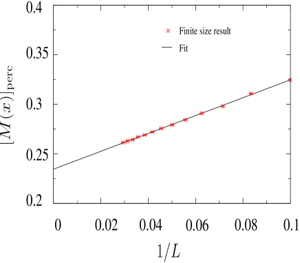
Figure 5: Staggered magnetization for the $t/U\rightarrow$ Heisenberg model for $x=20\%$ and $L\in[10,34]$.

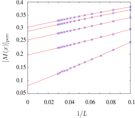
Figure 6: Evolution of $[M]_{\rm perc}$ for the $t/U\rightarrow$ Heisenberg model with $L$ for different values of dilution $-$ from top to bottom: $x=0\%$, $x=6\%$, $x=16\%$, $x=26\%$ and $x=36\%$.

Collecting these results, we show the staggered magnetization for the ground state of the site-diluted Heisenberg model, as a function of dilution in Fig. 7. $[M]_{\rm perc}$ goes smoothly from the known value for the undiluted case in the $1/S$ approximation Anderson (1952); Stinchcombe (1974); Manousakis (1991), $[M]_{\rm perc}\approx 0.31$, to zero for $x$ very close to the site dilution percolation threshold, $x_{p}$.

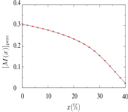
Figure 7: Staggered magnetization for the $t/U\rightarrow$ Heisenberg model on the percolating cluster extrapolated to the thermodynamic limit. The solid line is a guide to the eye.

In Fig. 8, we compare our result with those obtained by Mucciolo et al. Mucciolo et al. (2004) for the same model. The data are normalized by the value $[M]_{\rm perc}(x=0)\equiv M(0)$. There is extremely good quantitative agreement between our results and theirs, providing strong evidence that the two methods give correct results for the $1/S$ method considered.

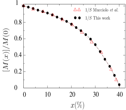
Figure 8: Comparison between our data for the ground state (bulk averaged) staggered magnetization for the Heisenberg model, normalized by the value at zero dilution, and the data of Mucciollo et al.Mucciolo et al. (2004) The dashed-dotted line is a guide to the eye.

It is important here to make a comparison between our results and those from quantum Monte Carlo (QMC), which is in principle exact, apart from numerical error. Such a comparison is made in Fig.  9 where we show unnormalized data for the magnetic moment on the percolation cluster from our calculation, compared with the QMC data of Ref. Sandvik, 2002. For zero dilution, the methods give very similar results. This is expected as it is known that $1/S^{2}$ contributions to the quantum fluctuations in this case are identically zero Stinchcombe (1974); Igarashi (1992); Igarashi and Nagao (2005), meaning that the difference between spin wave and QMC comes, to leading order, from $1/S^{3}$ contributions, which one might expect to be small. Moving away from zero dilution, the difference between the two sets of results increases in a monotonic way, with the moment from the QMC consistently larger than that determined from the $1/S$ spin wave calculation. Hence the comparison explicitly illustrates that the $1/S$ method over estimates the importance of the quantum fluctuations in the presence of disorder. In order to understand this quantitative difference, one should investigate the effects of magnon-magnon interactions and Berry phase terms, which we do not attempt here.

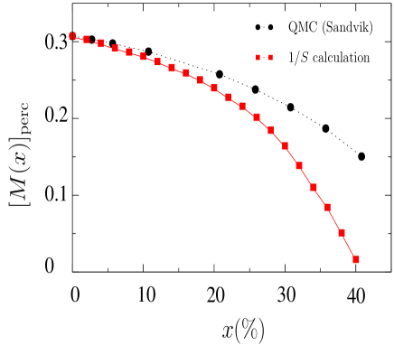
Figure 9: Staggered magnetization on the percolating cluster for the site-diluted Heisenberg model: comparison between QMC (from Ref. [Sandvik, 2002]) and $1/S$ spin wave results. The solid and dashed lines are guide to the eye.

The above limitations should be taken into consideration when comparing data from spin wave calculations with the experiment. In Fig. 10 we add our results to those previously shown in Fig. 1 for comparison with the experimental neutron scattering data on La₂Cu_1-x(Mg/Zn)_xO₄ Vajk et al. (2002) and quantum Monte Carlo simulations Sandvik (2002). The figure allows us to confirm the conclusion, already made in Ref. Mucciolo et al., 2004, that the extremely good agreement between experiment and the spin wave calculation is rather fortuitous: if the Heisenberg Hamiltonian was an adequate starting point to describe the experimental data, the “exact” QMC results would be in better agreement with the experimental data than the $1/S$ spin wave data are. As can be seen from the figure, the reverse is true; while the QMC data is consistently above the experimental curve, the spin wave data lies very close to it. Hence, although the Heisenberg Hamiltonian is clearly a good starting point for acquiring an acceptable qualitative description of Mg and Zn doped La₂CuO₄ it appears, on the basis of the results shown in Fig. 10, to be inadequate for a really quantitative description. Further, we remark that the experimental data are presented such that they are normalized by $[M(x=0)]_{\rm perc}$. While the undiluted moment is $[M(x=0)]_{\rm perc}\approx 0.31$ from QMC and spin wave calculations, recent estimates by Lee et al. Lee et al. (1999) place the experimental moment at about $0.25$. Hence, removing the absolute scale of the magnetic moment improves the impression of a good agreement of the experiment with the QMC results for the site-diluted Heisenberg model for small $x$. When plotted on an absolute scale the agreement between experiment and theory would be less convincing. This is an important point for the present paper as we continue to work within the linear spin wave approximation and cannot expect to account for the contributions beyond $1/S$ linear spin waves which, following the QMC approach, appear to be important for the dilution problem. That said, by making improvements to the starting spin-only description of the Hubbard Hamiltonian, through higher order terms in the canonical transformation, we can expect to improve the comparison with experiment on an absolute $[M(x)]$ scale.

With this in mind we have extended our calculations to order $t^{4}/U^{3}$, which allows us to include second and third neighbor exchange as well as ring exchange around an elementary plaquette, and also to include quantum fluctuations from charge delocalization in the underlying Hubbard model.

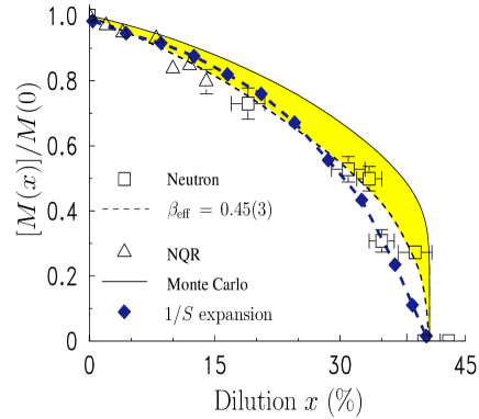
Figure 10: Ground state magnetization as a function of dilution for Mg and Zn doped La₂CuO₄: La₂Cu_1-x(Mg/Zn)_xO₄ Vajk et al. (2002), for quantum Monte Carlo Sandvik (2002) for the site-diluted square lattice Heisenberg antiferromagnet (SLHAF). The dashed line is a guide to the eye parameterized by $[M(x)]/M(0)=(1-x/x_{p})^{\beta_{\rm eff}}$. The figure is reproduced from Ref. [Vajk et al., 2002]. Added to this figure is our data and that of Ref. [Mucciolo et al., 2004] obtained from the numerical $1/S$ spin wave analysis of the site-diluted SLHAF.

.

IV.2 ${\mathbf{\mathit{missing}}t/U}\,=\,1/8$: on the role of the ring exchange interaction

When interactions beyond nearest neighbor exchange are taken into account, two effects have to be considered. First the transverse spin fluctuations are modified by the inclusion of the new interactions since these affect the magnon excitation spectrum Coldea et al. (2001); Delannoy et al. (2008). Secondly, the charge delocalization induces a further quantum fluctuation term over and above those from transverse spin fluctuations. This is the difference between $\hat{M}_{\rm s}$ and $\hat{\widetilde{M}}_{\rm s}$ in Eq. (20) and which leads to renormalization of the staggered magnetization in a way that depends on dilution. In this section, we treat these two effects separately to quantify their respective importance for $t/U\,=\,1/8$.

IV.2.1 In the absence of charge mobility renormalization

Finite size results:

The first point we wish to illustrate here is the importance of the modification of the exchange pathways in the diluted system. We have argued in Section (II.3) that dilution does not introduce random frustration at the classical level, even in the presence of further neighbor spin interactions, if these interactions are derived from the Hubbard model with nearest neighbor hops only. In this case, such a longer range interaction depends on the presence of a nearest neighbor exchange pathway. Hence, we do not expect long range interactions to have a destabilizing effect on classical Néel order on the percolating cluster. This can be seen indirectly by comparing the finite size scaling of our effective spin-only model with that of a more phenomenological model. In the latter, which we refer to as the “p-model”, the further neighbor interactions have full strength, independently of the existence of a nearest neighbor exchange path created by the electronic hopping processes, so that they exist even if the pathway is severed by a non-magnetic defect (i.e. diluted site). In the p-model, the bilinear exchange interactions $J_{2}$ and $J_{3}$ are taken to be $J_{2}=4t^{4}/U^{3}\epsilon_{i}\epsilon_{j}$ and $J_{3}=4t^{2}/U^{3}\epsilon_{i}\epsilon_{k}$ while $J_{c}$ is kept to have the same site occupancy dependence as in Eq. (12). In Fig. 11, we show results for the size dependence of the staggered magnetization $[{\widetilde{M}}]_{\rm perc}$ as a function of concentration $x$ of diluted sites. for the effective spin-only $H_{\rm s}^{(4)}$ in Eq. (II.1) with $\{J_{1},J_{2},J_{3},J_{c}\}$ coupling constants as given in Eqs. (9) to (12). The magnetization is a monotonic function of $L$ for all values of $x$. This should be compared with Fig. 12 where we show similar data for the p-model. For large dilution, the statistics are much worse and the magnetization considerably lower than in the first case. This indicates the build up of random frustrated plaquettes that eventually destroy the Néel order before $x_{p}$ is reached, even at the classical level Villain (1979); Binder et al. (1979); Parker and Saslow (1988); Saslow and Parker (1988); Vannimenus et al. (1989); Gawiec and Grempel (1991).

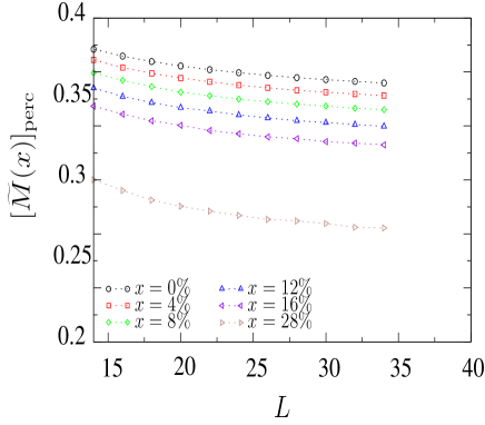
Figure 11: Size dependence of the staggered magnetization of the effective spin-only Hamiltonian $H_{\rm s}^{(4)}$. Further neighbor interactions are generated through the existence of nearest neighbor electronic hopping pathways. Charge mobility renormalization effects are not included here.

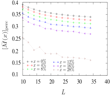
Figure 12: Size dependence of the staggered magnetization of a “p-model” Hamiltonian where further neighbor interactions are not explicitly dependent on the neighbor exchange hopping pathways.

Thermodynamic limit

For the effective spin-only Hamiltonian, results are extrapolated to the thermodynamic limit, using the procedure described in the previous section and Eq. (99). In Fig. 13 we show the ground state magnetization, $[{\widetilde{M}}]_{\rm perc}$, compared with the previously shown results from Fig. 7 for the ($t/U\rightarrow$, $J_{1}$ only) Heisenberg model.

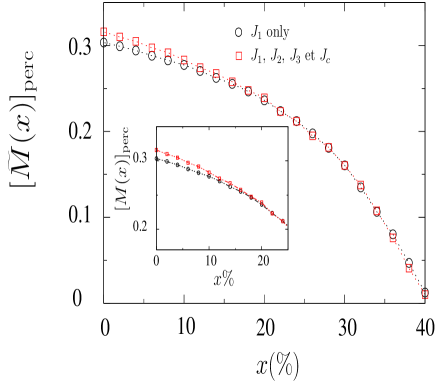
Figure 13: Dilution dependence of the staggered magnetization of the effective spin-only Hamiltonian obtained from the Hubbard model - No charge renormalization effect. The inset shows a blow-up for $x<20\%$.

The first thing to notice is that there is very little difference with the Heisenberg model! The second is that the small difference that is present is towards a higher ground state magnetization, with the maximum change occurring at $x\,=\,0\%$. This is because the ring exchange terms decrease the transverse spin fluctuations Delannoy et al. (2005, 2008). As discussed in Refs. [Delannoy et al., 2005, 2008], this increase in the magnetic moment occurs because the ring exchange terms in $H_{s}^{(4)}$ decouple in the $1/S$ expansion into effective ferromagnetic second neighbor two-body exchange terms which further stabilizes the two sublattice Néel order by reducing the transverse spin fluctuations Delannoy et al. (2005, 2008) (see Eq. (89)). For $x$ greater than about $12\%$ dilution, this stabilization effect is largely destroyed and the two curves merge up to the percolation threshold. This is explained by the fact that, as these interactions involve more than two sites, they are more sensitive to dilution than the nearest neighbor terms, and their effect becomes negligible long before the percolation threshold is reached. The effects at high dilution would be very different for the p-model (see Fig. 12) with frustrating further neighbor interactions that are independent of the presence of nearest neighbor exchange pathways. However, in the context of comparison with experimental results on La₂Cu_1-x(Mg/Zn)_xO₄, such terms should only appear through electronic hopping over further neighbors in the Hubbard model. We have recently considered this problem in the absence of dilution Delannoy et al. (2008), but extending this work to include dilution is beyond the scope of the present study.

IV.2.2 Finite charge mobility renormalization

The charge mobility, or electron delocalization effect, leads to a decrease in the magnetization Delannoy et al. (2005, 2008) (see Eq. (20)). However, the delocalization is also conditioned by the allowed nearest neighbor electronic hopping pathways and is consequently also dilution dependent. The finite size scaling of the magnetization, as described by Eq. (99), is not changed qualitatively by this renormalization (not shown here) and the results are extrapolated to the thermodynamic limit, using Eq. (99). As shown in Fig. 14, there is a significant decrease in the magnetization compared with $[{\widetilde{M}}]_{\rm perc}$ without charge mobility renormalization, or with the Heisenberg model (see Fig. 13). This difference is again reduced as the dilution increases. For $x=0\%$ the decrease is of the order of $14\%$, whereas it goes down to $9.5\%$ for $x=30\%$ and goes towards zero at the percolation threshold. We conclude therefore that the charge delocalization term is a major contribution to the corrections found by extending, to order $t^{4}/U^{3}$, the canonical transformation of the Hubbard model into an effective spin Hamiltonian. It is explicitly a property of the Hubbard model and is not present in a phenomenological spin-only model. It is therefore clear that care must be taken when using such phenomenological spin-only models without directly considering the mobility of the underlying system of electrons when aiming at obtaining a quantitative description and comparison between experiment and a microscopic theory. This is the main result of this paper.

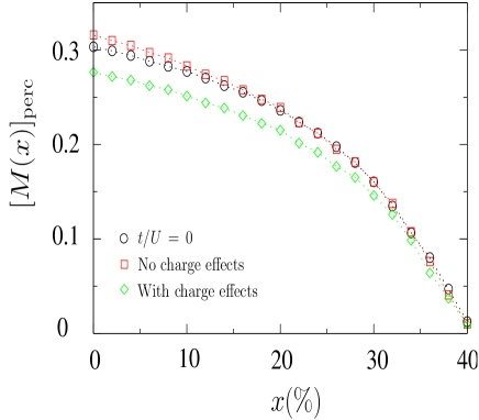
Figure 14: Evolution of the staggered magnetization with dilution for the effective spin-only Hamiltonian with charge mobility effects included. The open circles are the data for the Heisenberg ($t/U\rightarrow 0$) model. The diamonds and squares are respectively the data for the spin-only representation of the $t/U=1/8$ site-diluted Hubbard model with and without finite charge mobility renormalization included.

IV.3 Experimental considerations

Figure 14 illustrates our main result concerning the comparison with experiment: inclusion of the charge mobility renormalization factor shifts the scale of magnetization downwards over the whole dilution range. Comparing results for zero dilution; for the Heisenberg model, the ground state moment is $[M_{\rm s}]\approx 0.31$, while experiment yields $[M_{\rm s}]_{\rm exp}\approx 0.25$  Lee et al. (1999). Hence a comparison of $[M(x)]$ data not normalized by $M(x=0)$ will show the Heisenberg model, either from spin wave, or from QMC to be above those from the dilution experiments. Including hopping processes to order $t^{4}/U^{3}$ for $t/U=1/8$, a fair estimate for La₂CuO₄, one finds Coldea et al. (2001); Delannoy et al. (2008) $[M_{\rm s}]\approx 0.27$. This is still above the experimental value, but it is clear that, taken altogether, the extra corrections arising from both transverse spin fluctuations and finite electron mobility away from the $t/U\rightarrow 0$ Heisenberg limit, have scaled the magnetization in the right direction. This is an important result indicating that the perturbative methods proposed here can describe many of the magnetic features of La₂Cu_1-x(Mg/Zn)_xO₄.

In Fig. 15, we re-plot the data of Fig.  14 normalized by the ground state order parameter at zero dilution, $M(x=0)$. The two data sets for the Heisenberg model and that for the spin model $H_{s}^{(4)}$ with further neighbor interactions with the effects of electron delocalization via virtual hopping included, lie on top of each other. Hence, the improvements brought in by developing the effective spin description of the Hubbard model up to four virtual hopping terms, including ring exchange are not evident when the data are normalized in this way. The data sets would therefore continue to give the same favorable, but fortuitous comparison with the experimental data of Vajk et al. Vajk et al. (2002), as seen in Fig. 10 and discussed in Ref. [Mucciolo et al., 2004].

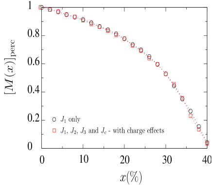
Figure 15: Data from Fig. 14 normalized by the ground state order parameter at zero dilution, $M(x=0)$.

V Conclusions and perspectives

V.1 Conclusions

In this paper we have investigated the problem of site dilution in systems described by the half-filled one-band Hubbard model. We have extended the canonical transformation technique to calculate an effective spin Hamiltonian up to order $t^{4}/U^{3}$, for magnetic site dilution $x$. We use a real space spin wave technique, linear in ($1/S$) to calculate the dilution dependence of quantum fluctuations on the staggered magnetization. Specifically, we considered two problems. We first studied the Heisenberg $t/U\rightarrow 0$ limit, comparing our results with those from quantum Monte Carlo (QMC) studies Sandvik (2002) on the same model. We confirm, to a high degree of accuracy, previous results from Ref. Mucciolo et al., 2004, using a similar $1/S$ technique. Hence, our results also confirm a systematic deviation between the QMC  Sandvik (2002) and the spin wave results for finite dilution. This difference, which is small for zero dilution, illustrates the dilution dependent generation of magnon-magnon interactions and Berry phase terms, both of which are neglected in the $1/S$ spin wave calculation. By comparing the QMC results and the $1/S$ results, one concludes that these two effects work to stabilize the semi-classical two sublattice Néel order rather than to drive the system into an exotic quantum phase. Hence, while the spin wave technique predicts the magnetic moment on the percolating cluster going to zero at, or very close to the percolation threshold, QMC simulations find a renormalized classical result, with the moment on the percolating cluster taking a discontinuous jump to zero at the percolation threshold.

The second and main objective of our work was to investigate how corrections to a site-diluted spin-only Hamiltonian, originating from a site-diluted one-band Hubbard model affects the dilution dependence of the Néel order parameter (staggered magnetization $[M(x)]$). Underlying this question, was the goal of obtaining some information on the capacity of the one-band Hubbard model to describe data from experiments on site-diluted La₂CuO₄, La₂Cu_1-x(Mg/Zn)_xO₄  Vajk et al. (2002).

Within the one-band Hubbard model, the best estimates from fitting to magnon excitation spectra Coldea et al. (2001); Delannoy et al. (2008) give $t/U\approx 1/8$, placing the system away from the Heisenberg limit and into the intermediate coupling regime, where higher order electron correlations need to be taken into account. Integrating out the kinetic degrees of freedom via a canonical transformation, implemented to order $t^{4}/U^{3}$, introduces second and third neighbor interactions into the resulting spin-only Hamiltonian, as well as ring exchange term from electronic pathways around a closed square plaquette. Calculation of the magnetization operator for the original Hubbard model, introduces at this order a charge mobility term that renormalizes the magnetization below that obtained by considering the (trivial) definition of the staggered magnetization of a spin-only Hamiltonian given by Eq. (21). Including all these effects, and staying within the linear ($1/S$) spin wave approximation, we find a reduced estimate for the moment at zero dilution, $\approx 0.27\mu_{\rm B}$ compared with $0.31\mu_{\rm B}$ for the Heisenberg model  Delannoy et al. (2005). As further neighbor and ring exchange interactions mediated by four electronic hops require unbroken exchange pathways over length scales greater than nearest neighbor, their effects disappear well before the percolation threshold is reached. The net result is therefore that the evolution of the ground state moment as a function of dilution is qualitatively similar to that for the Heisenberg model, disappearing at the percolation threshold in the same way, but with the absolute scale renormalized downwards by $10\%$ to $15\%$. While the $1/S$ method is subject to the limitations described above, our results clearly illustrate that for an ultimate detailed and quantitative understanding of the role of site dilution in a correlated electron system, such as La₂Cu_1-x(Mg/Zn)_xO₄, the charge mobility effects must be taken into account. Such a description is beyond a spin-only model, decoupled from an electronic model describing the behavior of the strongly correlated electrons.

V.2 Perspectives

To expand on the work presented in this paper, it would be interesting to carry out further theoretical and numerical studies using a common calculation scheme for both the site-diluted Hubbard model expressed in the framework of a spin-only Hamiltonian with ring exchange and the site-diluted Heisenberg ($t/U\rightarrow 0$) model. However, in the absence of a solution to the sign problem for frustrated quantum spin systems, quantitative results for the generalized dilution problem from large quantum Monte Carlo simulations remain inaccessible.

Angle resolved photo emission spectroscopic (ARPES) experiments as well as ab-initio calculations on a number of copper oxide materials provide strong evidence that an effective one-band Hubbard model description of these systems must include direct hopping parameters $t^{\prime}$ and $t^{\prime\prime}$ to second and third nearest neighbor sites. Furthermore, such experiments and calculations indicate that these parameters are not significantly smaller than the nearest neighbor hopping $t$, with $t^{\prime}/t\sim-0.3$ and $t^{\prime\prime}/t\sim 0.15$. We have recently included direct hopping parameters $t^{\prime}$ and $t^{\prime\prime}$ in a derivation of a spin-only Hamiltonian representation of the half-filled $t-t^{\prime}-t^{\prime\prime}-U$ Hubbard model Delannoy et al. (2008). As a result of these sizeable energy scales, our analysis of magnon excitation spectra in La₂CuO₄ reveal that the contributions from these parameters are of similar magnitude to the four hop (order $1/U^{4}$) processes for nearest neighbor hopping, which give rise to the ring exchange interactions studied in Ref. [Coldea et al., 2001] and in the present paper (last term in $H_{\rm s}^{(4)}$ of Eq. (II.1)).

A key result of Ref. [Delannoy et al., 2008] is that the ground state staggered moment, approximately 0.235, is further reduced from the value found for the $t-U$ Hubbard model, $\sim 0.27$, using the $t$ and $U$ values of Coldea et al. Coldea et al. (2001). This value is closer to, but undershoots the experimental estimate of $0.25$  Lee et al. (1999). Although this progression lies within the experimental uncertainty, the detailed analysis of Ref. [Delannoy et al., 2008] suggests that the $t-t^{\prime}-t^{\prime\prime}-U$ Hubbard model is a much improved starting point for a quantitative description of the magnetic properties of La₂CuO₄. This conclusion is in accordance with ARPES studies and ab-initio calculations on various cuprates.

A natural extension of the work presented in this paper would be to investigate the role of $t^{\prime}$ and $t^{\prime\prime}$ in the site dilution problem. In this model a large number of new ring exchange terms are generated and the further neighbor hopping terms allow for connected pathways for dilution concentrations above the nearest neighbor percolation threshold. It seems likely that these extra terms would change the shape of the $[M_{\rm s}(x)]$ vs $x$ curve, specially for $x$ close to $x_{p}$, and hence change the qualitative aspect of the results even when the magnetization scale is factorized out of the problem, as in Fig. 15.

The realization that $t^{\prime}$ and $t^{\prime\prime}$ are important energy scales in a Hubbard model description of La₂CuO₄ leads to an interesting experimental puzzle when considering the substitution of Cu²⁺ by non-magnetic Zn²⁺ and/or Mg²⁺. As discussed earlier in this paper, and as illustrated by the convergence of the the results of Fig. 13 for the Heisenberg model ($J_{1}$ only) and the $t/U=1/8$ Hubbard model ($J_{1}$, $J_{2}$, $J_{3}$ and $J_{c}$), the dilution-dependence of the electronic hopping pathways leads to a crossover concentration $x^{*}$ ($x^{*}\sim 15\%$ for $t/U=1/8$) above which the influence of the $J_{2}-J_{3}-J_{c}$ terms of order $1/U^{3}$ has essentially vanished. However, the presence of direct $t^{\prime}$ and $t^{\prime\prime}$ hoppings leads to additional frustrating second and third nearest neighbor exchange with $J_{2}^{\prime}\approx 4(t^{\prime})^{2}/U$ and $J_{3}^{\prime\prime}\approx 4(t^{\prime\prime})^{2}/U$, respectively. Unlike the $J_{2}$ and $J_{3}$ interactions generated by fourth order hopping processes, $J_{2}^{\prime}$ and $J_{3}^{\prime\prime}$ do not depend on the presence of nearest neighbor pathways and hence are unaffected by the dilution (see discussion in Section IV.2.1 and the one accompanying Fig. 12). As there is now frustration which is independent of the existence of nearest neighbor pathways, one would expect that upon dilution there would be a proliferation of Villain canted states Villain (1979); Binder et al. (1979); Parker and Saslow (1988); Saslow and Parker (1988); Vannimenus et al. (1989); Gawiec and Grempel (1991) as the concentration of impurities approaches the percolation threshold $x_{p}$. This could ultimately lead to a Heisenberg spin glass phase for a dilution concentration $x<x_{p}$. In this context, it is perhaps surprising that experiments find sharp (resolution limited) magnetic Bragg peaks in La₂Cu_1-x(Mg/Zn)_xO₄ all the way to $x=x_{p}$ Vajk et al. (2002). It would certainly be interesting to revisit this question and study in more detail the possibility of a spin glass phase developing in La₂Cu_1-x(Mg/Zn)_xO₄ close to the percolation threshold. We note further that in the region close to the percolation threshold there is the possibility of a freezing transition of the transverse spin components only. Such a transition could be observable in nuclear quadrupolar resonance (NQR) or muon spin relaxation (muSR) experiments Mirebeau et al. (1997) as were done sometime ago on La₂Cu_1-xZn_xO₄  Corti et al. (1995). However, in those early experiments Corti et al. (1995), it now seems likely that the then detected transverse spin freezing was driven by doped holes introduced by an imperfect control of the oxygen stoichiometry in La₂Cu_1-x(Mg/Zn)_xO₄  Vajk et al. (2002, 2003). It would be interesting to repeat such NQR and muSR experiments on La₂Cu_1-x(Mg/Zn)_xO₄ samples of the same quality as those used in neutron scattering experiments of Ref. [Vajk et al., 2002].

Another effect that could be relevant for La₂Cu_1-x(Mg/Zn)_xO₄ is the local distortion of the lattice due to the small difference in the ionic radius between Cu²⁺ and Mg²⁺ or Zn²⁺  Edagawa et al. (2007); Che . This difference could lead to a local modification of the hopping parameter $t$ in the neighborhood of a site where a Cu²⁺ ion is replaced by a nonmagnetic ion (see Fig. 2 in Ref. [Edagawa et al., 2007]). Such disorder-induced variations of the hopping parameters could then contribute to explain the difference between the experimental data and QMC data in Fig. 1. The importance of local distortions could perhaps be provided by local probe experiments such as muSR, NMR or NQR. This problem may also be considered as a precursor to the study of disorder-induced static magnetism in cuprate superconductors Anderson et al. (2007). In this case the inclusion of mobile holes makes it much more complicated, but the study of the diamagnetic dilution problem in La₂Cu_1-x(Mg/Zn)_xO₄ maintained at half filling could provide a useful framework on which to build.

In conclusion, we have explored in this work the problem of the evolution of the magnetic order in a spin-only representation of a site-diluted one-band Hubbard expressed in terms of a spin-only Hamiltonian, taking into account up to four hop processes. For a finite ratio of hopping constant to on-site Coulomb energy, $t/U$, the resulting spin Hamiltonian differs from the simpler site-diluted $S=1/2$ Heisenberg model, containing effective exchange coupling beyond nearest neighbor as well as ring exchange interactions. The long range exchange interactions, the ring exchange and the renormalization of the nearest neighbor exchange depend specifically on the local random hopping pathways that remain uninterrupted by the missing (diluted) sites. We hope that this study can motivate further analytical and numerical studies of the site-diluted one-band Hubbard model as well as new experiments on La₂Cu_1-x(Mg/Zn)_xO₄ in the vicinity of the percolation threshold.

VI Acknowledgements

It is a pleasure to thank A.-M. S. Tremblay for a related collaboration leading to the publications of Ref. [Delannoy et al., 2005, 2008] as well as for useful comments on this manuscript. We also thank G. Albinet, B. Castaing, A. Castro Neto, F. Delduc, T. Devereaux, A. Mucciolo, L. Raymond, A. Sandvik, R. Scalettar, O. Vajk and T. Vojta for useful discussions. Partial support for this work was provided by NSERC of Canada and the Canada Research Chair Program (Tier I) (M.G.) Research Corporation and the Province of Ontario (M.G.) and a Canada$-$France travel grant from the French Embassy in Canada (M.G.and P.H.). M.G. acknowledges the Canadian Institute for Advanced Research (CIFAR) for support.

Appendix A Calculation procedure for the Bogoliubov transformation

We summarize below the steps required to obtain the eigenvector matrix for $\tilde{H}$, $\widetilde{E}$ satisfying the boson commutation relations (39):

• Diagonalize $\tilde{H}$ using the Lapack routines. This yields a set of eigenvalues $\omega_{i}$ with corresponding eigen-subspaces generated by the eigenvectors $E_{i}^{n}$, where $n\in\{1,p_{i}\}$ and where $p_{i}$ is the degeneracy of the eigenvalue and dimension of the subspace.

• For the subspace $i$ define $E_{i}$, a $2N\times p_{i}$ matrix of the corresponding eigenvectors $E_{i}^{n}$. Form the block matrix $M_{i}$

  $$M_{i}\,=\,E_{i}^{{\dagger}}\tilde{I}E_{i},$$ (101)

  of size $p_{i}\times p_{i}$.

• Invert $M_{i}$ to get $M_{i}^{-1}$.

• Diagonalize $M_{i}^{-1}$, thus defining $K_{i}$ and $D_{i}$:

  $$M_{i}^{-1}\,=\,K_{i}D_{i}K_{i}^{-1}.$$ (102)

• Define the matrix:

  $$A_{i}\,=\,K_{i}\sqrt{\pm D_{i}}K_{i}^{-1}.$$ (103)

  In this expression, the sign $\pm$ corresponds to the sign of $\omega_{i}$.

• Define the new matrix of eigenvectors for the subspace $i$, $\tilde{E_{i}}$:

  $$\tilde{E_{i}}\,=\,E_{i}A_{i}.$$ (104)

• Repeat subspace by subspace to construct the eigenvector matrix $\widetilde{E}$.

Appendix B Statistical errors

this section we discuss the origin of the statistical errors we find from our numerical results. Consider, as an example, the lattice of size $L^{2}\,=\,24\times 24$. For $x\,=\,12\%$, we studied ${\cal N}_{0}=620$ different realizations of disorder. The average magnetization and root mean square (RMS) variation, $\Delta M$, were found to be

$$[M(x=12\%,L=24)]_{\rm perc}\,=\,0.305\;,\Delta M=0.0052$$ (105)

from which we estimate the error on the measure to be $\pm\sigma_{M(x)}$  Boas (1983)

$$\sigma_{M(x)}={\mathchoice{\dfrac{\Delta M_{\rm s}}{{\sqrt{{{\cal N}_{0}}}}}}{\dfrac{\Delta M_{\rm s}}{{\sqrt{{{\cal N}_{0}}}}}}{\frac{\Delta M_{\rm s}}{{\sqrt{{{\cal N}_{0}}}}}}{\frac{\Delta M_{\rm s}}{{\sqrt{{{\cal N}_{0}}}}}}}.$$ (106)

In this example the estimated error is thus extremely small, around $0.1\%$ and the errors rise to around $1\%$ near the percolation threshold. This small error estimate is consistent with the statistical fluctuations observed in Figs. 5 and 7.

For the example considered above, the ratio of the dispersion to the mean value:

$${\mathchoice{\dfrac{\Delta M}{[M]_{\rm perc}}}{\dfrac{\Delta M}{[M]_{\rm perc}}}{\frac{\Delta M}{[M]_{\rm perc}}}{\frac{\Delta M}{[M]_{\rm perc}}}}\,=\,1.705\%.$$ (107)

The ratio of the dispersion, $\Delta M$, to mean value $[M]_{\rm perc}$, for fixed dilution $L$ as a function of $x$ and for fixed $x$ and as a function of $L$ are shown in Tables (1) and (2), respectively.

$x(\%)$	$[M]_{\rm perc}$	$\Delta M$	${\mathchoice{\dfrac{\Delta M}{[M]_{\rm perc}}}{\dfrac{\Delta M}{[M]_{\rm perc}}}{\frac{\Delta M}{[M]_{\rm perc}}}{\frac{\Delta M}{[M]_{\rm perc}}}}(\%)$
0	$0.338$	$0$	$0$
2	$0.334$	$0.0014$	$0.419$
4	$0.329$	$0.0022$	$0.668$
6	$0.324$	$0.0028$	$0.864$
8	$0.319$	$0.0036$	$1.128$
10	$0.313$	$0.0041$	$1.310$
12	$0.305$	$0.0052$	$1.705$
14	$0.298$	$0.0060$	$2.013$
16	$0.290$	$0.0070$	$2.414$
18	$0.281$	$0.0080$	$2.847$
20	$0.272$	$0.0096$	$3.529$
22	$0.261$	$0.0109$	$4.176$
24	$0.249$	$0.0135$	$5.421$
26	$0.236$	$0.0154$	$6.525$
28	$0.221$	$0.0183$	$8.281$
30	$0.204$	$0.0213$	$10.440$
32	$0.186$	$0.0237$	$12.742$
34	$0.166$	$0.0274$	$16.506$
36	$0.147$	$0.0291$	$19.795$
38	$0.125$	$0.0316$	$25.280$
40	$0.109$	$0.0330$	$30.275$

Table 1: Staggered magnetization for $L^{2}=24\times 24$ and $x\in[0,40]\%$

$L$	$[M]_{\rm perc}$	$\Delta M$
10	0.325	0.0181
12	0.311	0.0166
14	0.298	0.0160
16	0.291	0.0134
18	0.284	0.0118
20	0.279	0.0114
22	0.276	0.0103
24	0.272	0.0096
26	0.269	0.0090
28	0.267	0.0079
30	0.264	0.0080
32	0.263	0.0075
34	0.261	0.0068

Table 2: Staggered magnetization for $x=20\%$ and $L\in[10,34]$.

We can model this dispersion using three sources of variation: firstly, for a given $x$ the number of magnetic sites varies from configuration to configuration. Secondly, for fixed $N$ the number of sites on the percolating cluster will also vary. Thirdly, there will also be a contribution from configurational fluctuations for a fixed number of sites. We stress that all these contributions are quantum in origin. That is, the classical ground state is perfectly ordered for all concentrations above the percolation threshold, as discussed in the main text, hence at the classical level, changing the number of sites, or local structures on the percolating cluster will not change the order parameter. However, the dilution reduces the local spin stiffness for spins in contact with non-magnetic sites and increases the zero point spin fluctuations. Hence these variations in number of sites and structure change the value of the order parameter. Indeed this point is already manifest by the fact that $[M]_{\rm perc}$ decreases with $x$.

If $N_{i}(L^{2},x)$ is the number of sites for realization $i$, and the mean number of sites is defined in Eq. (98) then for the example considered we find

$$\bar{N}(L=24,x=12\%)\,=\,506.8\pm 7.7.$$ (108)

Hence

$${\mathchoice{\dfrac{\Delta\bar{N}}{\bar{N}}}{\dfrac{\Delta\bar{N}}{\bar{N}}}{\frac{\Delta\bar{N}}{\bar{N}}}{\frac{\Delta\bar{N}}{\bar{N}}}}\,=\,1.51\%.$$ (109)

To check the importance of fluctuations in the number of participating sites on the percolating cluster, $(N_{\rm perc})_{i}$ we analyze the ratio ${\mathchoice{\dfrac{(N_{\rm perc})_{i}}{N_{i}}}{\dfrac{(N_{\rm perc})_{i}}{N_{i}}}{\frac{(N_{\rm perc})_{i}}{N_{i}}}{\frac{(N_{\rm perc})_{i}}{N_{i}}}}$. We find

$${\mathchoice{\dfrac{N_{\rm perc}}{N}}{\dfrac{N_{\rm perc}}{N}}{\frac{N_{\rm perc}}{N}}{\frac{N_{\rm perc}}{N}}}\,=\,0.999\pm 6.67\times 10^{-3}~{},$$ (110)

which gives

$${\mathchoice{\dfrac{\Delta{\mathchoice{\dfrac{N_{\rm perc}}{N}}{\dfrac{N_{\rm perc}}{N}}{\frac{N_{\rm perc}}{N}}{\frac{N_{\rm perc}}{N}}}}{{\mathchoice{\dfrac{N_{\rm perc}}{N}}{\dfrac{N_{\rm perc}}{N}}{\frac{N_{\rm perc}}{N}}{\frac{N_{\rm perc}}{N}}}}}{\dfrac{\Delta{\mathchoice{\dfrac{N_{\rm perc}}{N}}{\dfrac{N_{\rm perc}}{N}}{\frac{N_{\rm perc}}{N}}{\frac{N_{\rm perc}}{N}}}}{{\mathchoice{\dfrac{N_{\rm perc}}{N}}{\dfrac{N_{\rm perc}}{N}}{\frac{N_{\rm perc}}{N}}{\frac{N_{\rm perc}}{N}}}}}{\frac{\Delta{\mathchoice{\dfrac{N_{\rm perc}}{N}}{\dfrac{N_{\rm perc}}{N}}{\frac{N_{\rm perc}}{N}}{\frac{N_{\rm perc}}{N}}}}{{\mathchoice{\dfrac{N_{\rm perc}}{N}}{\dfrac{N_{\rm perc}}{N}}{\frac{N_{\rm perc}}{N}}{\frac{N_{\rm perc}}{N}}}}}{\frac{\Delta{\mathchoice{\dfrac{N_{\rm perc}}{N}}{\dfrac{N_{\rm perc}}{N}}{\frac{N_{\rm perc}}{N}}{\frac{N_{\rm perc}}{N}}}}{{\mathchoice{\dfrac{N_{\rm perc}}{N}}{\dfrac{N_{\rm perc}}{N}}{\frac{N_{\rm perc}}{N}}{\frac{N_{\rm perc}}{N}}}}}}\,=\,0.6\%~{}.$$ (111)

For a fixed number of magnetic sites, we can define the quantity

$$\left({\mathchoice{\dfrac{\Delta M}{[M]_{\rm perc}}}{\dfrac{\Delta M}{[M]_{\rm perc}}}{\frac{\Delta M}{[M]_{\rm perc}}}{\frac{\Delta M}{[M]_{\rm perc}}}}\right)_{\rm mag}$$

as a measure of the configurational contribution to the dispersion in ground state order parameter values, where $\left(\dots\right)_{\rm mag}$ is the disorder average over the restricted set of configurations with $N_{i}=constant$. For the example discussed here we find

$$\left({\mathchoice{\dfrac{\Delta M}{[M]_{\rm perc}}}{\dfrac{\Delta M}{[M]_{\rm perc}}}{\frac{\Delta M}{[M]_{\rm perc}}}{\frac{\Delta M}{[M]_{\rm perc}}}}\right)_{\rm mag}\,=\,0.4677\%~{},$$ (112)

from which we estimate the total dispersion

$$\left({\mathchoice{\dfrac{\Delta M}{[M]_{\rm perc}}}{\dfrac{\Delta M}{[M]_{\rm perc}}}{\frac{\Delta M}{[M]_{\rm perc}}}{\frac{\Delta M}{[M]_{\rm perc}}}}\right)_{\rm tot}\,=\,{\mathchoice{\dfrac{\Delta\bar{N}}{\bar{N}}}{\dfrac{\Delta\bar{N}}{\bar{N}}}{\frac{\Delta\bar{N}}{\bar{N}}}{\frac{\Delta\bar{N}}{\bar{N}}}}+{\mathchoice{\dfrac{\Delta{\mathchoice{\dfrac{N_{\rm perc}}{N}}{\dfrac{N_{\rm perc}}{N}}{\frac{N_{\rm perc}}{N}}{\frac{N_{\rm perc}}{N}}}}{{\mathchoice{\dfrac{N_{\rm perc}}{N}}{\dfrac{N_{\rm perc}}{N}}{\frac{N_{\rm perc}}{N}}{\frac{N_{\rm perc}}{N}}}}}{\dfrac{\Delta{\mathchoice{\dfrac{N_{\rm perc}}{N}}{\dfrac{N_{\rm perc}}{N}}{\frac{N_{\rm perc}}{N}}{\frac{N_{\rm perc}}{N}}}}{{\mathchoice{\dfrac{N_{\rm perc}}{N}}{\dfrac{N_{\rm perc}}{N}}{\frac{N_{\rm perc}}{N}}{\frac{N_{\rm perc}}{N}}}}}{\frac{\Delta{\mathchoice{\dfrac{N_{\rm perc}}{N}}{\dfrac{N_{\rm perc}}{N}}{\frac{N_{\rm perc}}{N}}{\frac{N_{\rm perc}}{N}}}}{{\mathchoice{\dfrac{N_{\rm perc}}{N}}{\dfrac{N_{\rm perc}}{N}}{\frac{N_{\rm perc}}{N}}{\frac{N_{\rm perc}}{N}}}}}{\frac{\Delta{\mathchoice{\dfrac{N_{\rm perc}}{N}}{\dfrac{N_{\rm perc}}{N}}{\frac{N_{\rm perc}}{N}}{\frac{N_{\rm perc}}{N}}}}{{\mathchoice{\dfrac{N_{\rm perc}}{N}}{\dfrac{N_{\rm perc}}{N}}{\frac{N_{\rm perc}}{N}}{\frac{N_{\rm perc}}{N}}}}}}+\left({\mathchoice{\dfrac{\Delta M}{[M]_{\rm perc}}}{\dfrac{\Delta M}{[M]_{\rm perc}}}{\frac{\Delta M}{[M]_{\rm perc}}}{\frac{\Delta M}{[M]_{\rm perc}}}}\right)_{\rm mag}\simeq 2\%~{}.$$ (113)

in good agreement with Eq. (107). The analysis can be generalized to the other values of $x$ and $L$. For example for $L^{2}=24\times 24$ and $x\,=\,30\%$ we have:

$$\left\{\begin{array}[]{ccl}{\mathchoice{\dfrac{\Delta\bar{N}}{\bar{N}}}{\dfrac{\Delta\bar{N}}{\bar{N}}}{\frac{\Delta\bar{N}}{\bar{N}}}{\frac{\Delta\bar{N}}{\bar{N}}}}&=&3.48\%~{},\\ \\ {\mathchoice{\dfrac{\Delta{\mathchoice{\dfrac{N_{\rm perc}}{N}}{\dfrac{N_{\rm perc}}{N}}{\frac{N_{\rm perc}}{N}}{\frac{N_{\rm perc}}{N}}}}{{\mathchoice{\dfrac{N_{\rm perc}}{N}}{\dfrac{N_{\rm perc}}{N}}{\frac{N_{\rm perc}}{N}}{\frac{N_{\rm perc}}{N}}}}}{\dfrac{\Delta{\mathchoice{\dfrac{N_{\rm perc}}{N}}{\dfrac{N_{\rm perc}}{N}}{\frac{N_{\rm perc}}{N}}{\frac{N_{\rm perc}}{N}}}}{{\mathchoice{\dfrac{N_{\rm perc}}{N}}{\dfrac{N_{\rm perc}}{N}}{\frac{N_{\rm perc}}{N}}{\frac{N_{\rm perc}}{N}}}}}{\frac{\Delta{\mathchoice{\dfrac{N_{\rm perc}}{N}}{\dfrac{N_{\rm perc}}{N}}{\frac{N_{\rm perc}}{N}}{\frac{N_{\rm perc}}{N}}}}{{\mathchoice{\dfrac{N_{\rm perc}}{N}}{\dfrac{N_{\rm perc}}{N}}{\frac{N_{\rm perc}}{N}}{\frac{N_{\rm perc}}{N}}}}}{\frac{\Delta{\mathchoice{\dfrac{N_{\rm perc}}{N}}{\dfrac{N_{\rm perc}}{N}}{\frac{N_{\rm perc}}{N}}{\frac{N_{\rm perc}}{N}}}}{{\mathchoice{\dfrac{N_{\rm perc}}{N}}{\dfrac{N_{\rm perc}}{N}}{\frac{N_{\rm perc}}{N}}{\frac{N_{\rm perc}}{N}}}}}}&=&1.41\%~{},\\ \\ \left({\mathchoice{\dfrac{\Delta M}{[M]_{\rm perc}}}{\dfrac{\Delta M}{[M]_{\rm perc}}}{\frac{\Delta M}{[M]_{\rm perc}}}{\frac{\Delta M}{[M]_{\rm perc}}}}\right)_{\rm mag}&=&5.45\%~{},\end{array}\right.$$ (114)

which correspond to $\left({\mathchoice{\dfrac{\Delta M}{[M]_{\rm perc}}}{\dfrac{\Delta M}{[M]_{\rm perc}}}{\frac{\Delta M}{[M]_{\rm perc}}}{\frac{\Delta M}{[M]_{\rm perc}}}}\right)_{\rm tot}\simeq 10\%$, as obtained in Table 1. Hence this analysis seems to account for the dispersion in magnetization values to a good level of approximation. The three sources of dispersion are of the same order of magnitude as long as one remains well away from the percolation threshold. At low defect concentration (small $x$) it is the fluctuations in the number of magnetic sites that dominates. As $x$ increases the fluctuations increase, as one might expect as one approaches the critical percolating regime, and at large $x$ it is the configurational contribution for fixed particle number which dominates. At $40\%$ dilution the dispersion in values approaches $30\%$ of the mean order parameter value. Despite this large dispersion for this value of $x$ the number of configurations, ${\cal N}_{0}=2000$, is large enough to keep the estimated error at the $1\%$ level.

References

- Grinstein (1985) G. Grinstein, in Fundamental Problems in Statistical Mechanics VI, proceeding of the Sixth International Summer School, Trondheim, Norway, 1984, edited by E. G. D. Cohen (North-Holland, Amsterdam, 1985).
- Ill (1979) in Ill-Condensed Matter (Ecole D’été de Physique Théoretique Les Houches, 3 July - 18 August 1978, edited by R. Balian, R. Maynard, and G. Toulouse (North-Holland,Amsterdam, 1979).
- Harris (1974) A. Harris, J. Phys. C 7, 1671 (1974).
- Imry and Ma (1975) Y. Imry and S.-K. Ma, Phys. Rev. Lett. 35, 1399 (1975).
- Binder and Young (1986) K. Binder and A. P. Young, Rev. Mod. Phys. 58, 801 (1986).
- Anderson (1987) P. W. Anderson, Science 235, 1196 (1987).
- Sachdev (2008) S. Sachdev, Nature Physics 4, 173 (2008).
- Shender and Kivelson (1991) E. F. Shender and S. A. Kivelson, Phys. Rev. Lett. 66, 2384 (1991).
- Eggert and Affleck (2004) S. Eggert and I. Affleck, J. Mag. Magn. Mater. 272, Suppl. E647 (2004).
- Sirker et al. (2008) J. Sirker, S. Fujimoto, N. Laflorencie, S. Eggert, and I. Affleck, J. Stat. Mech. P02015 (2008).
- Azuma et al. (1997) M. Azuma, Y. Fujishiro, M. Takano, M. Nohara, and H. Takagi, Phys. Rev. B 55, R8658 (1997).
- Wessel et al. (2001) S. Wessel, B. Normand, M. Sigrist, and S. Haas, Phys. Rev. Lett. 86, 1086 (2001).
- Sandvik and Vekic (1995) A. W. Sandvik and M. Vekic, Phys. Rev. Lett. 74, 1226 (1995).
- Yu et al. (2006) R. Yu, T. Roscilde, and S. Haas, Phys. Rev. B 73, 064406 (2006).
- Ghosh et al. (2003) S. Ghosh, T. F. Rosenbaum, G. Aeppli, and S. N. Coppersmith, Nature 425, 48 (2003).
- Metlitski and Sachdev (2007) W. M. Metlitski and S. Sachdev, Phys. Rev. B 76, 064423 (2007).
- Chakraborty et al. (1989) A. Chakraborty, A. J. Epstein, and M. Jarrell, Phys. Rev. B 40, 5296 (1989).
- Cheong et al. (1991) S. W. Cheong, A. S. Cooper, L. W. Rupp, B. Batlogg, J. D. Thompson, and Z. Fisk, Phys. Rev. B 44, 9739 (1991).
- Wan et al. (1991) C. C. Wan, A. B. Harris, and J. Adler, J. Appl. Phys. 69, 5191 (1991).
- Corti et al. (1995) M. Corti, A. Rigamonti, F. Tabak, P. Carretta, F. Licci, and L. L. Raffo, Phys. Rev. B 52, 4226 (1995).
- Villain (1979) J. Villain, Z. Phys. B 33, 31 (1979).
- Binder et al. (1979) K. Binder, W. Kinzel, and D. Stauffer, Z. Phys. B 36, 161 (1979).
- Parker and Saslow (1988) G. N. Parker and W. M. Saslow, Phys. Rev. B 38, 11718 (1988).
- Saslow and Parker (1988) W. M. Saslow and G. N. Parker, Phys. Rev. B 38, 11733 (1988).
- Vannimenus et al. (1989) J. Vannimenus, S. Kirkpatrick, F. D. M. Haldane, and C. Jayaprakash, Phys. Rev. B 39, 4634 (1989).
- Gawiec and Grempel (1991) P. Gawiec and D. R. Grempel, Phys. Rev. B 44, 2613 (1991).
- Chernyshev et al. (2002) A. L. Chernyshev, Y. C. Chen, and A. H. Castro Neto, Phys. Rev. B 65, 104407 (2002).
- Kato et al. (2000) K. Kato, S. Todo, K. Harada, N. Kawashima, S. Miyashita, and H. Takayama, Phys. Rev. Lett. 84, 4204 (2000).
- Sandvik (2002) A. W. Sandvik, Phys. Rev. B 66, 024418 (2002).
- Vajk et al. (2002) O. P. Vajk, P. K. Mang, M. Greven, P. M. Gehring, and J. W. Lynn, Science 295, 1691 (2002).
- Vajk et al. (2003) O. P. Vajk, M. Greven, P. K. Mang, and J. W. Lynn, Sol. St. Comm. 126, 93 (2003).
- Notbohm et al. (2007) S. Notbohm, P. Ribeiro, B. Lake, D. A. Tennant, K. P. Schmidt, G. S. Uhrig, C. Hess, R. Klingeler, G. Behr, B. Büchner, et al., Phys. Rev. Lett. 98, 027403 (2007).
- Gößling et al. (2003) A. Gößling, U. Kuhlmann, C. Thomsen, A. Löffert, C. Gross, and W. Assmus, Phys. Rev. B 67, 052403 (2003).
- Roger (2005) M. Roger, J. Phys. Chem. Solids 66, 1412 (2005).
- Coldea et al. (2001) R. Coldea, S. M. Hayden, G. Aeppli, T. G. Perring, C. D. Frost, T. E. Mason, S.-W. Cheong, and Z. Fisk, Phys. Rev. Lett. 86, 5377 (2001).
- Toader et al. (2005) A. M. Toader, J. P. Goff, M. Roger, N. Shannon, J. R. Stewart, and M. M. Enderle, Phys. Rev. Lett. 94, 197202 (2005).
- Raymond et al. (2006) L. Raymond, G. Albinet, and A.-M. S. Tremblay, Phys. Rev. Lett. 97, 049701 (2006).
- Toader et al. (2006) A. M. Toader, J. P. Goff, M. Roger, N. Shannon, J. R. Stewart, and M. M. Enderle, Phys. Ref. Lett. 97, 049702 (2006).
- MacDonald et al. (1988) A. H. MacDonald, S. Girvin, and D. Yoshioka, Phys. Rev. B 37, 9753 (1988).
- Chernyshev et al. (2004) A. L. Chernyshev, D. Galanakis, P. Phillips, A. V. Rozhkov, and A.-M. S. Tremblay, Phys. Rev. B 70, 235111 (2004).
- Delannoy et al. (2005) J.-Y. P. Delannoy, M. J. P. Gingras, P. C. W. Holdsworth, and A.-M. S. Tremblay, Phys. Rev. B 72, 115114 (2005).
- Melko and Kaul (2008) R. G. Melko and R. K. Kaul, Phys. Rev. Lett. 100, 017203 (2008).
- Walker and Waldstedt (1980) L. R. Walker and R. E. Waldstedt, Phys. Rev. B 22, 3816 (1980).
- Mucciolo et al. (2004) A. R. Mucciolo, A. H. Castro Neto, and C. Chamon, Phys. Rev. B 69, 214424 (2004).
- Castro et al. (2006) E. V. Castro, N. M. R. Peres, K. S. D. Beach, and A. W. Sandvik, Phys. Rev. B 73, 054422 (2006).
- Delannoy et al. (2008) J.-Y. P. Delannoy, M. J. P. Gingras, P. C. W. Holdsworth, and A.-M. S. Tremblay, unpublished (2008).
- Harris and Lange (1967) A. B. Harris and R. V. Lange, Phys. Rev. 157, 295 (1967).
- MacDonald et al. (1990) A. H. MacDonald, S. Girvin, and D. Yoshioka, Phys. Rev. B 41, 2565 (1990).
- MacDonald et al. (1991) A. H. MacDonald, S. Girvin, and D. Yoshioka, Phys. Rev. B 43, 6209 (1991).
- Chandra and Doucot (1988) P. Chandra and B. Doucot, Phys. Rev. B 38, 9335 (1988).
- Dagotto and Moreo (1989) E. Dagotto and A. Moreo, Phys. Rev. Lett. 63, 2148 (1989).
- Young (1995) A. P. Young, in Les Houches 1991 Session LVI Strongly interacting fermions and high Tc superconductivity, edited by B. Dou ot and J. Zinn-Justin (North Holland, 1995).
- Chubukov et al. (1992) A. Chubukov, E. Gagliano, and C. Balseiro, Phys. Rev. B 45, 7889 (1992).
- (54) J. Y. Delannoy, Ph.D. thesis, ENS-Lyon (2005).
- (55) A recent study Delannoy et al. (2008) that incorporates the efect of second () and third () nearest neighbor oppings also find that a value allows for a spin-only Hamiltonian whose magnon excitations suitably describe the spin-waves of La2CuO4 Coldea et al. (2001).
- Huse (1987) D. A. Huse, Phys. Rev. B 37, 2380 (1987).
- Anderson (1952) P. W. Anderson, Phys. Rev. 86, 694 (1952).
- Stinchcombe (1974) R. B. Stinchcombe, J. Phys. C 4, 789 (1974).
- Manousakis (1991) E. Manousakis, Rev. Mod. Phys. 63, 1 (1991).
- Igarashi (1992) J.-I. Igarashi, Phys. Rev. B 46, 10763 (1992).
- Igarashi and Nagao (2005) J.-I. Igarashi and T. Nagao, Phys. Rev. B 72, 014403 (2005).
- Lee et al. (1999) Y. S. Lee, R. J. Birgeneau, K. M. A., E. Y., S. Wakimoto, K. Yamada, R. W. Erwin, S.-H. Lee, and G. Shirane, Phys. Rev. B 60, 3643 (1999).
- Mirebeau et al. (1997) I. Mirebeau, M. Hennion, M. J. P. Gingras, A. Keren, K. Kojima, M. Larkin, G. M. Luke, B. Nachumi, W. D. Wu, Y. J. Uemura, et al., Hyper. Int. 104, 343 (1997).
- Edagawa et al. (2007) T. Edagawa, Y. Fukumoto, and A. Oguchi, J. Magn. Mag. Mater. 310, e406-e408 (2007).
- (65) We note that S. Liu and S. Chernyshev have also explored how local impurities such as Mg2+ and Zn2+ in La2CuO4 can lead to some local random frustration. See http://meetings.aps.org/Meeting/MAR06/Event/43205 and http://meetings.aps.org/Meeting/MAR07/Event/58199 .
- Anderson et al. (2007) B. M. Anderson, P. J. Hirschfeld, A. P. Kampf, and M. Schmid, Phys. Rev. Lett. 99, 147002 (2007).
- Boas (1983) M. Boas, Mathematical Methods in the Physical Sciences (Wiley, 1983).